Cyberphysical System Modeled with Complex Networks and Hybrid Automata to Diagnose Multiple and Concurrent Faults in Manufacturing Systems

Abstract

Cyber–physical systems use digital twins to provide advanced monitoring and control functions, including self-diagnosis. The digital twin is often conceptualized as a 3D model, but mathematical models implemented in numerical simulations are required to reproduce the dynamical and functional characteristics of physical systems. In this work, a cyber–physical system scheme is proposed to monitor and diagnose failures. The virtual system, embedded at the supervisory control level, combines concepts from complex networks and hybrid automata to detect failures in the hardware components and in the execution of the sequential logic control. An automated storage and retrieval system is presented as a case study to show the applicability of the proposed scheme. The functional test and the obtained results validate the implemented system that is shown to be capable of fault diagnosis and location in real time. The online execution of the digital twin present several advantages for diagnosing multiple concurrent failures in sensors, actuators, and the control unit. This approach can be incorporate into diverse manufacturing systems.

1. Introduction

Over the years, the industry has had changes in terms of the technology implemented to improve and produce more with fewer human resources; we can see this in the so-called industrial revolutions. The last revolution is Industry 4.0, which emphasizes the use of digital technology developed in the third industrial revolution, but takes it to a more advanced level with the help of interconnectivity through the Internet of Things (IoT), access to data in real time and the introduction of cyber–physical systems. An existing problem in these systems is that, due to their complexity in the occurrence of faults, their diagnosis and location are very complex, which motivates this research work.

Cyber–physical systems are integrated by two subsystems: a physical system composed of sensors, actuators, Programmable Logic Controllers (PLC), and in some cases, a human–machine Interface (HMI) [1,2,3], and a digital system that is considered a part of the systems that develop different tasks such as the monitoring, optimization and diagnosis of the physical system [4,5,6]. The digital system in the project comprises a supervisory controller, fault diagnosis component and digital twin. Additionally, a communication protocol to send/receive information in both subsystems is needed. In cyberphysical systems, a mathematical tool called hybrid automata is used that provides the possibility of modeling digital and analog variables and allows the use of time delays that are important for the system to communicate with its digital twin [7,8,9]. The cyber–physical systems (CPS) must be in real-time communication to be able to verify information about the process.

Among the different possibilities for the operation of the digital Twin inside a CPS, which is a widely accepted approach, the Digital Twin provides a means for the remote and simulated commissioning of manufacturing systems, thus allowing for the rapid reconfiguration of the automated manufacturing system. In contrast, the presented CPS approach is oriented for fault detection, which requires the Digital Twin to run in parallel with the physical systems. The run-time execution and comparison may allow multiple and concurrent fault detection. In the application of Industry 4.0, there exist possibilities to propose, design and implement new concepts that may improve production systems, which is of interest to both academia and the industry.

We found in [10,11,12] that the combination of hybrid automata and complex network theory has been applied for system analysis but not for diagnosing system failures. A complex network can reproduce the evolution of a networked system if the system is controlled by a hybrid automata that changes from one state to another [13]. The hybrid control system activates or deactivates actuators in response to sensor values. Adjacency matrices are constructed for the analysis of complex networks, which places correspondences to the connected nodes [14,15,16]. From the reading of sensors and the activation and deactivation of actuators of the physical system, information is saved in the adjacency matrix using arbitrary weights, corresponding to the space assigned by each sensor or actuator [17].

In the present work, a functional and practical approach to a cyber–physical system is presented to diagnose multiple concurrent failures in an automatic storage and retrieval system. The virtual twin comprises a hybrid automata and a numerical simulation of the physical system. Sensors, actuators, and control units, as connected devices, are modeled as complex networks to take advantage of some concepts and analysis tools derived from complex networks theory. The objective of the proposed cyber–physical system approach is to monitor and diagnose failures in the sensors and actuators and in the execution of the sequential logic control. The digital twin is embedded in the supervisory controller and is executed simultaneously with the physical process. The application of the computational algorithms is to detect failures in a timely manner and thus reduce delays in manufacturing production processes, and improve productivity. This paper is organized as follows: Section 2 recalls some concepts of cyberphysical systems, hybrid automata, and complex networks. In Section 3, the material and methods, the proposed scheme and the results are presented. Section 4 discusses the results of the implemented CPS scheme and the challenges in its implementation. Section 5 is the conclusion and future work.

2. Background

This section describes the theoretical background required for the conceptualization of a cyber–physical system. This includes definitions of cyber–physical systems, hybrid systems, hybrid automata, complex networks, and analysis tools.

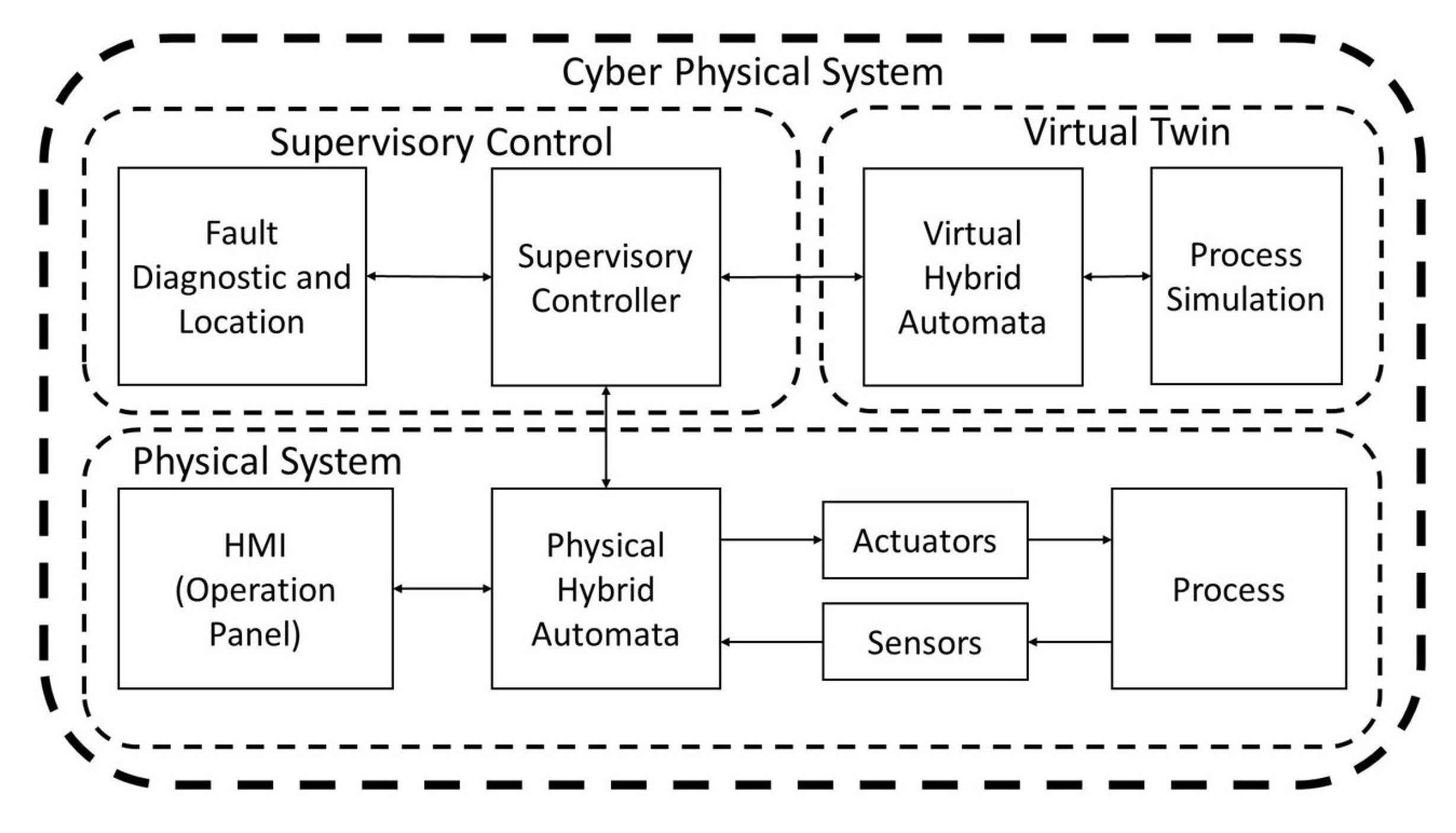
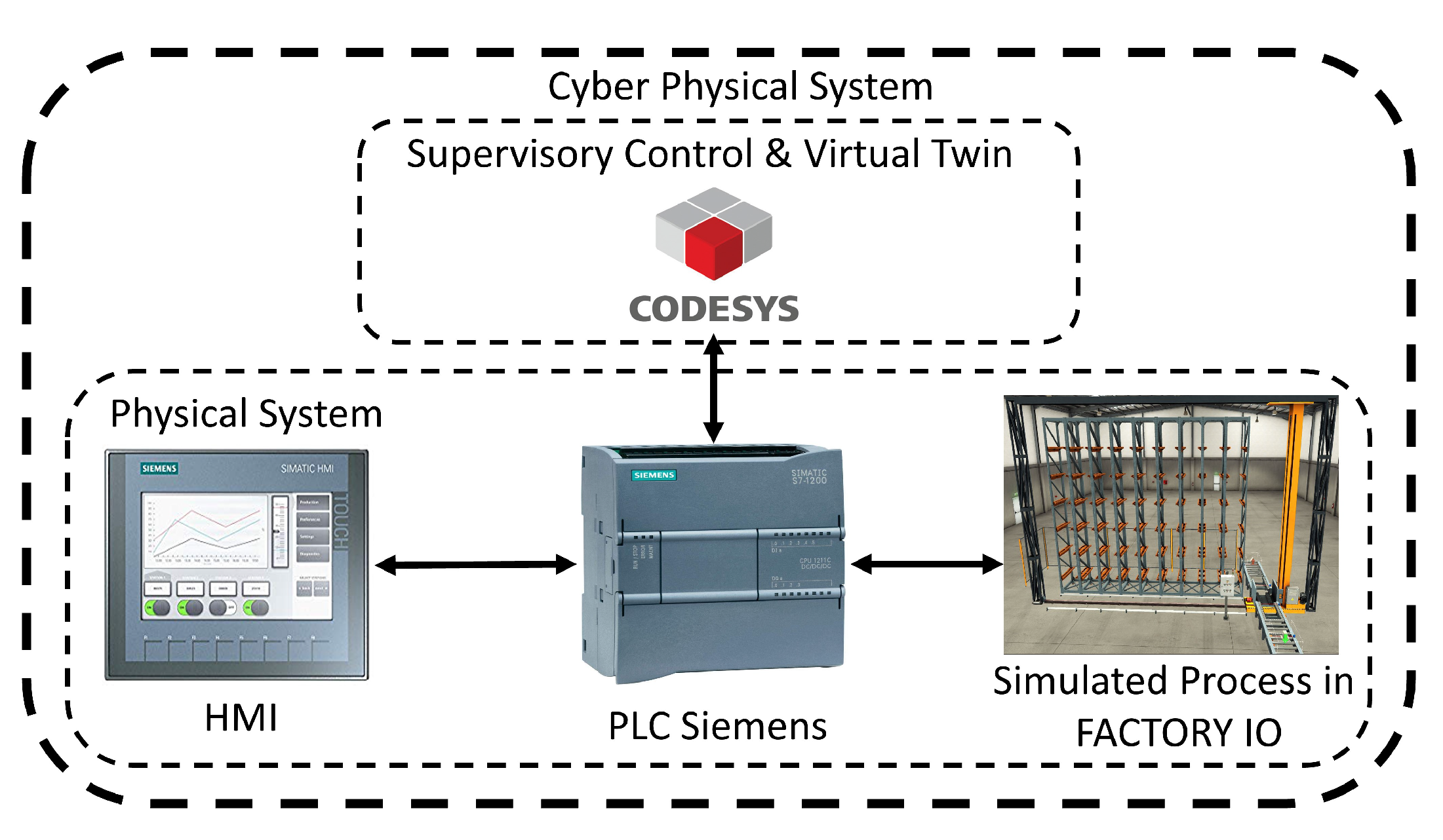
2.1. Cyber–Physical Systems

A cyber–physical system (CPS) refers to a system with combined computational and physical capabilities, as it interacts with users through new modalities. The ability to communicate and expand the operations of the physical world through computer technology, interaction, and control are aspects of high importance in technological development. Autonomous cars, hybrid or fully electric vehicles, the design and development of aircrafts, and remotely controlled manufacturing systems represent research challenges and opportunities. In the control area, progress has been made in the implementation of engineering methods and tools, such as the linear control, discrete control, optimization, prediction, filtering, time and frequency domain, and state space analysis. In the area of computer systems, progress has been made in technological advances such as information security and system failure detection, reliability innovation, integrated software and new computer system architectures, visualization procedures, and real-time simulation techniques, based on models and new simulation languages. The development of cyber–physical systems aims to integrate the behavior of a physical system in the computing and engineering areas (mechatronics, software, human interaction, artificial intelligence, as well as chemical and material sciences and other engineering disciplines) to develop new systems’ CPS [18].

2.2. Hybrid Systems

Hybrid systems are characterized by continuous and discrete dynamics, since in these systems, logical decision making and regulatory control actions are combined with continuous physical processes. Mathematical models should combine the continuous and discrete dynamics of the system. Such mathematical models consist of differential or difference equations of continuous dynamics and automata or other discrete event models for discrete dynamics. The combination of modeling techniques is the basis of hybrid systems theory, which plays an important role in the multidisciplinary design of many cyber–physical systems [19].

2.3. Hybrid Automata

Hybrid automata provide formal models for hybrid dynamical systems and can be observed as an extension of finite automata by adding continuous dynamics into each of its discrete states (also called modes). Each mode is associated with constraints, within which the continuous dynamics evolve. Edges between modes are annotated with guards that specify the conditions for the mode transition to be triggered; each edge is also associated with a reset map indicating how the continuous variables are being updated after the discrete transition. Hybrid automata are defined below [19].

A hybrid automaton H is a collection:

$$\begin{array}{c}\hfill H=\left(Q,X,f,Init,Inv,E,G,R\right)\end{array}$$

where:

$Q=(q1,q2,\dots )$ is a finite set of discrete states;

$X\subseteq R^n$ represents the state space of the continuous state variables;

$f:QxX\to R^n$ assigns to each discrete state $q\in Q$ an analytic vector field $f(q,·);$

$Init\subseteq QxX$ is the set of initial states;

$Inv:Q\to 2^x$ assigns to each state $q\in Q$ a set $Inv\left(q\right)\subseteq X$ called the invariant set;

$E\subseteq QxQ$ is the set of discrete transitions;

$G:E\to 2^x$ assigns to each discrete transition $(q,q^{\prime })\in E$ a guard set $G(q,q^{\prime })\subset X$;

$R:ExX\to 2^x$ is a reset map.

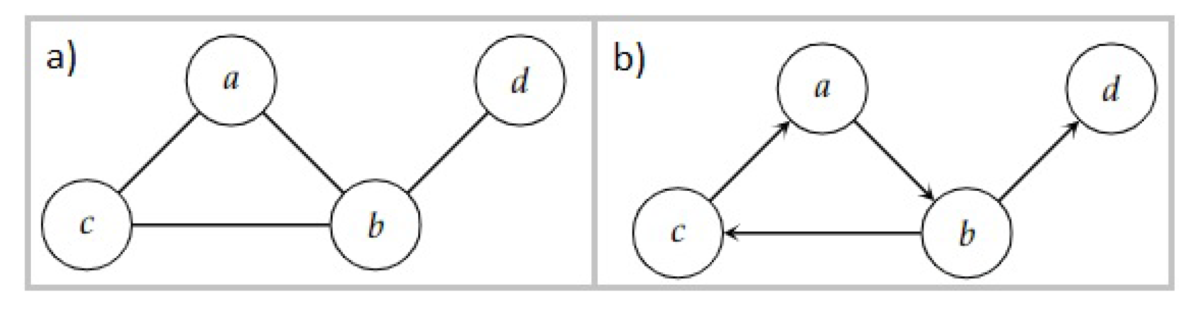
2.4. Complex Networks

Complex networks are known as sets of interconnected nodes. The nodes of a network can be called vertices or elements and are represented by the symbols $v_1,v_2,\cdots ,v_N$, where N is the total number of nodes in the network. If a node $v_i$ is connected to another node $v_j$, this connection is represented by an ordered pair $(v_i,v_j)$. The mathematical definition of a network (also called a graph) is as follows: Formally, a network R consists of a set of nodes $V=v_1,v_2,\dots V_N$ and a set of ordered pairs $E=(v_i,v_j)\subset VxV$. Each ordered pair $(v_i,v_j)$ is a directed connection from node $v_i$ to node $v_j$. A non-directed type network consists of that for each pair $(v_i,v_j)\in \epsilon$ there also exists the pair $(v_j,v_i)\in \epsilon$, as shown in Figure 1a. If the above is not fulfilled, the network directed, as Figure 1b. Illustrates. Nodes that are directly connected to a $v_i$ node are called $v_i$’s neighbors [20].

3. Matherial and Methods

Most of the proposed approaches for fault diagnostic using DT and CPS are more oriented for commissioning manufacturing systems for reconfiguration and optimization purposes. The proposed approach differs from that found in the literature, since the DT is required to run in parallel to be able to perform an online fault Diagnostics. In this section, a basic conceptualization of a cyber–physical system incorporating a complex network is presented.

3.1. Cyber–Physical System Components

The cyber–physical system proposed here is composed by a communication structure between two systems, physical and digital systems. The physical system comprises a programmable logic controller (PLC), and a human–machine interface (HMI) interconnected to the supervisory controller through the PLC. The digital system comprises a supervisory control and a digital twin embedded in the digital system. The complete proposed CPS scheme is shown in the diagram of Figure 2.

In the proposed cyber–physical system, there are two automata: $H_P$, which is the physical hybrid automata, and $H_V$, that is, the hybrid virtual automata, which is executed in a virtual system. $T_S$ is the synchronization time and $Ad{j}_M$ is the Adjacency Matrix.

$$CPS=\{H_P,H_V,T_S,Ad{j}_M\}$$

The hybrid automatas $H_F$ and $H_V$ share the same sets of states, functions and variables; however, the $H_V$ variables are from the virtual system and the $H_P$ variables from the physical system. The graphic representation of the automata is presented in Figure 3 and Figure 4.

$$Q=\{q0,q1,q2,q3,q4,q5,q6,q7,q8,q9\}$$

$$dx=Rdenotestherangeofthecurrentbasedintheoutputsactivatedx=\alpha *y_{n-1}+(1-\alpha )y_n$$

$$Init=\left\{q0\right\}x\left\{1\right\}or\left\{q10\right\}x\left\{1\right\}$$

$$f(q0,x1)=10andf(q1,x2)=10andf(q2,x3,x4,x5)=5,5,10and$$

$$f(q3,x6,x7)=2,10andf(q4,x8,x9,x10,x11)=2,2,10,10andf(q5,x12,x13)=2,10,and$$

$$f(q6,x14,x15)=2,10,andf(q7,x16,x17,x18)=2,2,10andf(q8,x19,x20)=2,10,and$$

$$f(q9,x21)=10andf(q10,x22)=10and(q11,x23)=10,andf(q12,x24)=10and$$

$$f(q13,x25)=10,andf(q14,x26)=2,andf(q15,x27,X28)=2,10,and$$

$$f(q16,x29,x30)=2,10,andf(q17,x31,x32)=2,10and$$

$$f(q18,x33,x34,x35,x36,x37)=5,5,2,2,10andf(q19,x38,x39,x40)=5,5,10and$$

$$f(q20,x41,x42,x43)=5,5,10andf(q21,x44,x45,x46)=5,5,10$$

$$Inv\left(q0\right)=\{x\in R:x\ge 10\}andInv\left(q1\right)=\{x\in R:x\ge 10\}and$$

$$Inv\left(q2\right)=\{x\in R:x\ge 20\}andInv\left(q3\right)=\{x\in R:x\ge 12\}and$$

$$Inv\left(q4\right)=\{x\in R:x\ge 24\}andInv\left(q5\right)=\{x\in R:x\ge 12\}and$$

$$Inv\left(q6\right)=\{x\in R:x\ge 12\}andInv\left(q7\right)=\{x\in R:x\ge 14\}and$$

$$Inv\left(q8\right)=\{x\in R:x\ge 12\}andInv\left(q9\right)=\{x\in R:x\ge 10\}and$$

$$Inv\left(q10\right)=\{x\in R:x\ge 10\}andInv\left(q11\right)=\{x\in R:x\ge 10\}and$$

$$Inv\left(q12\right)=\{x\in R:x\ge 10\}andInv\left(q13\right)=\{x\in R:x\ge 10\}and$$

$$Inv\left(q14\right)=\{x\in R:x\ge 2\}andInv\left(q15\right)=\{x\in R:x\ge 12\}and$$

$$Inv\left(q16\right)=\{x\in R:x\ge 12\}andInv\left(q17\right)=\{x\in R:x\ge 12\}and$$

$$Inv\left(q18\right)=\{x\in R:x\ge 24\}andInv\left(q19\right)=\{x\in R:x\ge 20\}$$

$$Inv\left(q20\right)=\{x\in R:x\ge 20\}andInv\left(q21\right)=\{x\in R:x\ge 20\}$$

$$E1=\left\{\right(q0,q12\left)\right(q0,q1),(q1,q2\left)\right(q2,q3\left)\right(q3,q4\left)\right(q4,q5)$$

$$(q5,q6)(q6,q7)(q7,q8)(q8,q9)(q9,q10)(q10,q11)\}$$

$$E2=\left\{\right(q12,q0\left)\right(q12,q13),(q13,q14\left)\right(q14,q15\left)\right(q15,q16\left)\right(q16,q17)$$

$$(q17,q18)(q18,q19)(q19,q20)(q20,q21)(q21,q12)\}$$

$$G(q0,q1)=\{x\in R:x1\ge 9.8\}andG(q1,q2)=\{x\in R:x2\ge 9.8\}and$$

$$G(q2,q3)=\{x\in R:x3\ge 19.8\}andG(q3,q4)=\{x\in R:x4\ge 11.8\}and$$

$$G(q4,q5)=\{x\in R:x5\le 23.8\}andG(q5,q6)=\{x\in R:x6\le 11.8\}and$$

$$G(q6,q7)=\{x\in R:x7\le 11.8\}andG(q7,q8)=\{x\in R:x8\ge 13.8\}and$$

$$G(q8,q9)=\{x\in R:x9\ge 11.8\}andG(q9,q10)=\{x\in R:x1\ge 9.8\}and$$

$$G(q10,q11)=\{x\in R:x1\ge 9.8\}andG(q11,q0)=\{x\in R:x1\ge 9.8\}$$

$$G(q0,q12)=\{x\in R:x1\ge 9.8\}$$

$$G(q12,q13)=\{x\in R:x2\ge 9.8\}andG(q13,q14)=\{x\in R:x3\ge 9.8\}and$$

$$G(q14,q15)=\{x\in R:x4\ge 1.8\}andG(q15,q16)=\{x\in R:x5\ge 11.8\}and$$

$$G(q16,q17)=\{x\in R:x6\ge 11.8\}andG(q17,q18)=\{x\in R:x7\ge 11.8\}and$$

$$G(q18,q19)=\{x\in R:x8\ge 23.8\}andG(q19,q20)=\{x\in R:x9\ge 19.8\}$$

$$G(q20,q21)=\{x\in R:x8\ge 19.8\}andG(q21,q12)=\{x\in R:x9\ge 19.8\}$$

$$G(q12,q0)=\{x\in R:x8\ge 9.8\}$$

$$R\left(\right(q0,q1),x)=\left\{x\right\}andR\left(\right(q1,q2),x)=\left\{x\right\}andR\left(\right(q2,q3),x)=\left\{x\right\}and$$

$$R\left(\right(q3,q4),x)=\left\{x\right\}andR\left(\right(q4,q5),x)=\left\{x\right\}andR\left(\right(q5,q6),x)=\left\{x\right\}and$$

$$R\left(\right(q6,q7),x)=\left\{x\right\}andR\left(\right(q7,q8),x)=\left\{x\right\}andR\left(\right(q8,q9),x)=\left\{x\right\}and$$

$$R\left(\right(q9,q0),x)=\left\{x\right\}andR\left(\right(q10,q11),x)=\left\{x\right\}andR\left(\right(q11,q12),x)=\left\{x\right\}and$$

$$R\left(\right(q12,q13),x)=\left\{x\right\}andR\left(\right(q13,q14),x)=\left\{x\right\}andR\left(\right(q14,q15),x)=\left\{x\right\}and$$

$$R\left(\right(q15,q16),x)=\left\{x\right\}andR\left(\right(q16,q17),x)=\left\{x\right\}andR\left(\right(q17,q18),x)=\left\{x\right\}and$$

$$R\left(\right(q18,q19),x)=\left\{x\right\}andR\left(\right(q19,q10),x)=\left\{x\right\}$$

$$Ad{j}_{MInputs}=\{V_{I1},V_{I2},V_{I3},V_{I4},V_{I5},V_{I6},V_{I7},V_{I8},V_{I9},$$

$$V_{I10},V_{I11},V_{I12},V_{I13},V_{I14},V_{I15},V_{I16},V_{I17}\}$$

$$Ad{j}_{MOutputs}=\{V_{O1},V_{O2},V_{O3},V_{O4},V_{O5},V_{O6},V_{O7},V_{O8},V_{O9},$$

$$V_{O10},V_{O11},V_{O12},V_{O13},V_{O14},V_{O15},V_{O16},V_{O17}\}$$

$T_S$ = The synchronization time will depend on the supervisory control. For the proposed system, a time delay of 100 ms is considered for each state change to compare the input and output vectors.

3.2. Cyber–Physical System Implementation

Within the industry, engineering-based system design has been characterized by separating the control system from the construction features of hardware and software. Once the control of the system is completed, a complete simulation is usually performed to verify the optimal operation and correct uncertainty in the model, as well as external disturbances not considered in the model. An important characteristic of industrial systems is their increasing complexity due to the use of advanced technologies for instrumentation, communication and multilevel information processing, posing an important challenge to design and build future generation industrial manufacturing systems. In the design and construction of cyber–physical systems, a new methodology is needed that leads to a reliable and optimal integration of the system elements that were designed independently. The proposed system can be implemented for testing with a programmable logic controller (PLC) and a human–machine interface (HMI). To simulate the process, a graphic environment is used to reproduce the operation of the automatic storage system, Figure 5. The digital system is implemented on a codesys soft plc that incorporates the digital twin and the online diagnostic functions based upon the complex network.

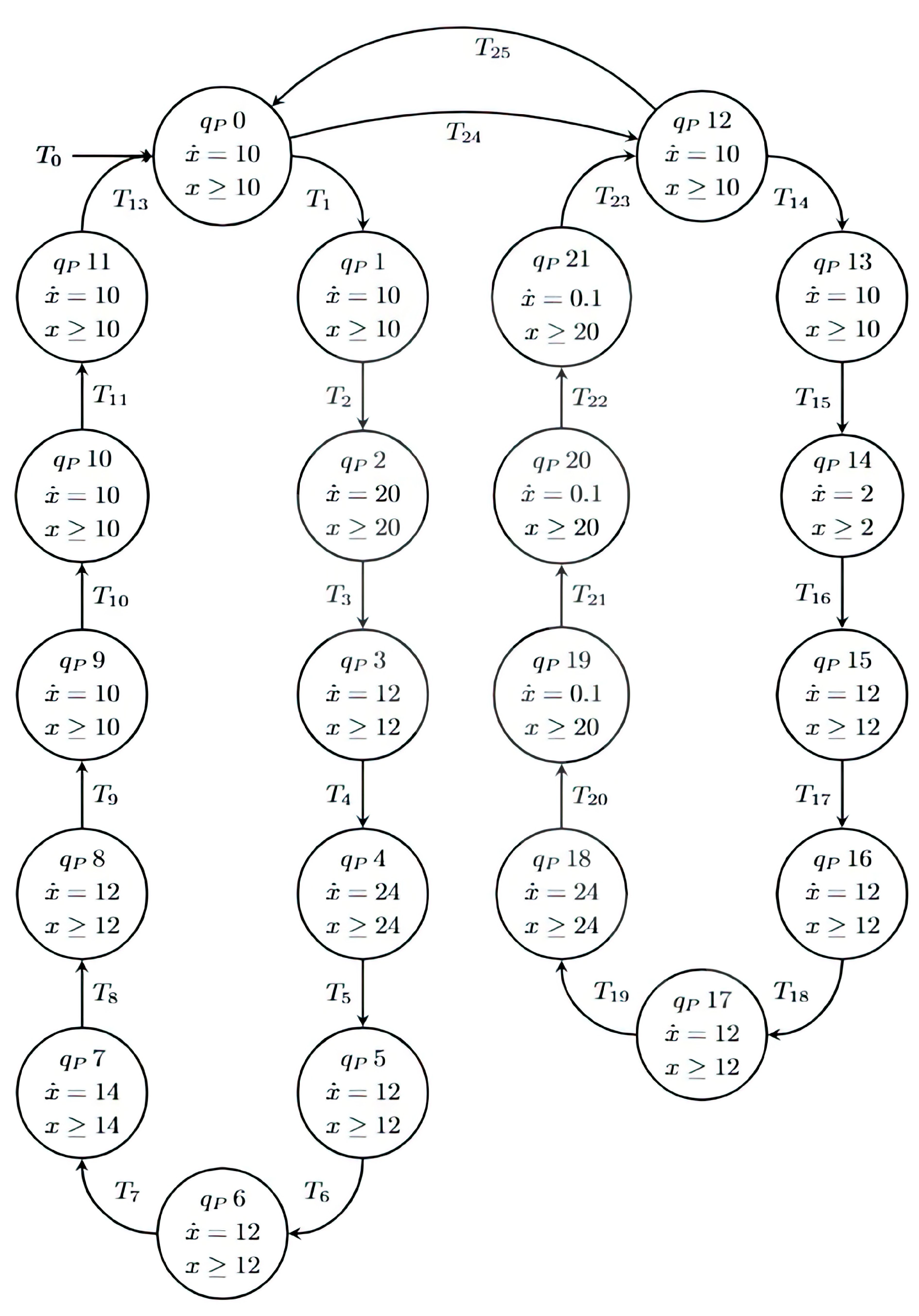
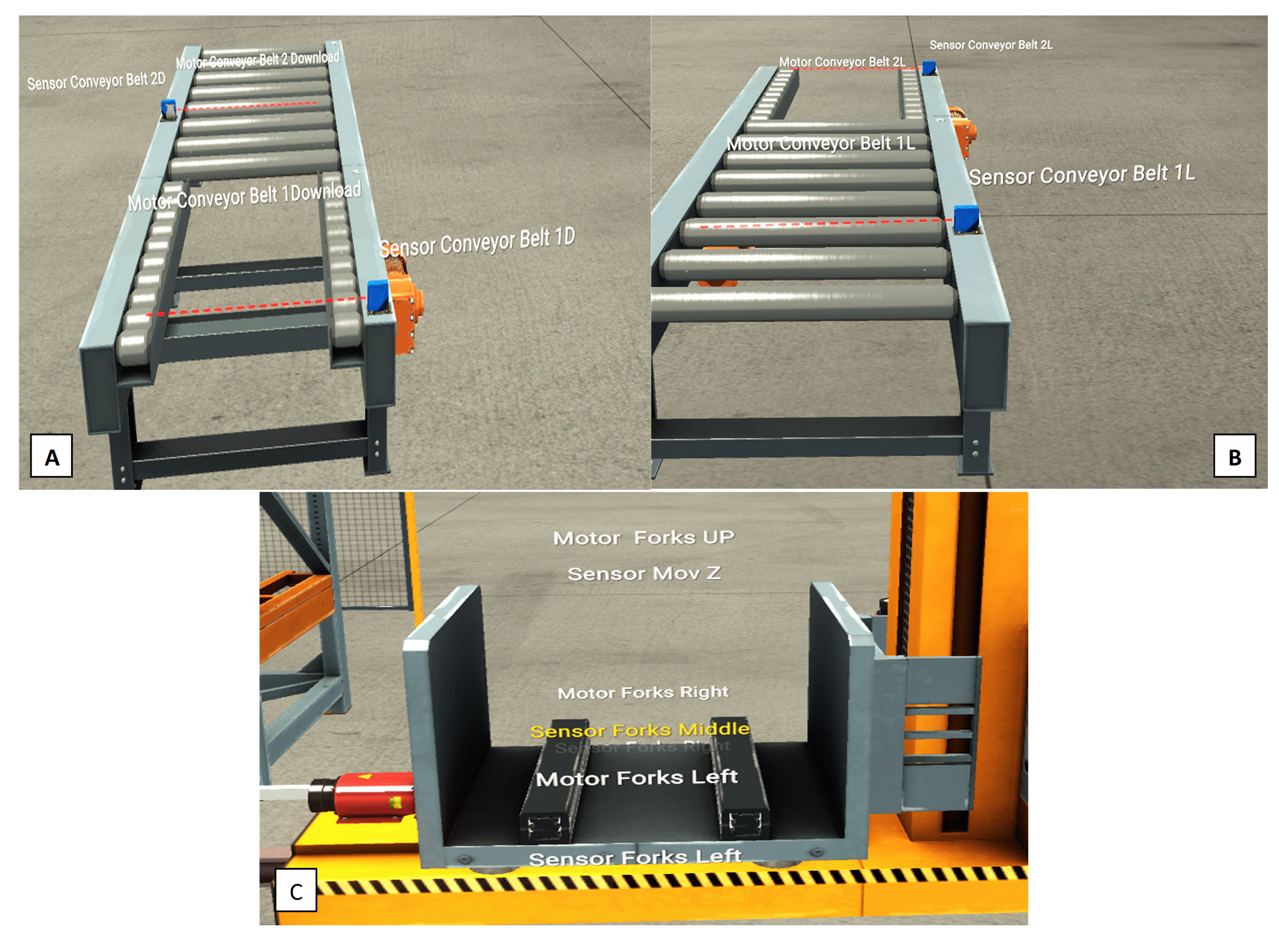
3.3. Physical Hybrid Model of Warehouse Operation

The operation of an automatic warehouse is modeled as an hybrid automaton. The states of the physical system are divided into two modes of operation: loading and filling the warehouse and unloading and emptying the warehouse. In addition, the variable that will be measured is the current consumed by the actuators activated in each state. The loading mode of the elevator has the following programming, the $q_{P0}$ status activates the indicator lights of the buttons and the light column, state $q_{P1}$ activates two belt motors that transport the product for storage, state $q_{P2}$ activates the movement of the forks to the left, state $q_{P3}$ activates the movement of the forks upwards, state $q_{P4}$ activates the movement of the forks retracting to the left, state $q_{P5}$ activates an elevator that carries the package to a specific position, state $q_{P6}$ activates the movement of the forks to the right, state $q_{P7}$ activates the movement of the forks retracting from the top, state $q_{P8}$ activates the movement of the forks retracting to the right, state $q_{P9}$ is the elevator sent to its home position, state $q_{P10}$ is the elevator in the home position, and state $q_{P11}$ is the delay time for the system in Figure 6B,C. The hardware configuration of the system can be observed.

The unloading mode has the following programming, as shown in Figure 6A,C: State $q_{P12}$ activates the indicator lights of the buttons and the light column, state $q_{P13}$ activates the elevator that goes to the unloading position, state $q_{P14}$ activates the movement of the forks to the right, state $q_{P15}$ activates the movement of the forks upwards, state $q_{P16}$ activates the movement of the forks to the right retractor, state $q_{P17}$ is the elevator sent to its home position, state $q_{P18}$ is the movement of the forks to the right being activated, state $q_{P19}$ is the movement of the forks retracting downwards being activated, state $q_{P20}$ is the movement of the forks retracting to the right being activated, and state $q_{P21}$ is the elevator being sent home, as well as the conveyor belts that remove the object from the warehouse being activated. Figure 3 shows the automaton and

Table 1. State and Output Activation.

State	Output	State	Output	State	Output	State	Output
$q_{P0}$	Leds 1	$q_{P5}$	Elevator motors (QW30)	$q_{P10}$	Leds 1	$q_{P15}$	Elevator motors
$q_{P1}$	Conveyor Motors (Q10.6, Q10.7)	$q_{P6}$	Motor forks (Q11.0 Right)	$q_{P11}$	Elevator motors	$q_{P16}$	Motor forks
$q_{P2}$	Motor forks (Q11.1 Left)	$q_{P7}$	Motor forks (Q11.2 Up)	$q_{P12}$	Motor forks	$q_{P17}$	Motor forks
$q_{P3}$	Motor forks (Q11.2 Up)	$q_{P8}$	Motor forks (Q11.0 Right)	$q_{P13}$	Motor forks	$q_{P18}$	Motor forks
$q_{P4}$	Motor forks (Q11.1 LeftR)	$q_{P9}$	Elevator motors (QW30)	$q_{P14}$	Motor forks	$q_{P19}$	Conveyor motor

¹ Led Outputs = Q10.0, Q10.1, Q11.3, Q10.2, Q10.3, Q11.4, Q10.3.

shows the states and outputs activated in each one.

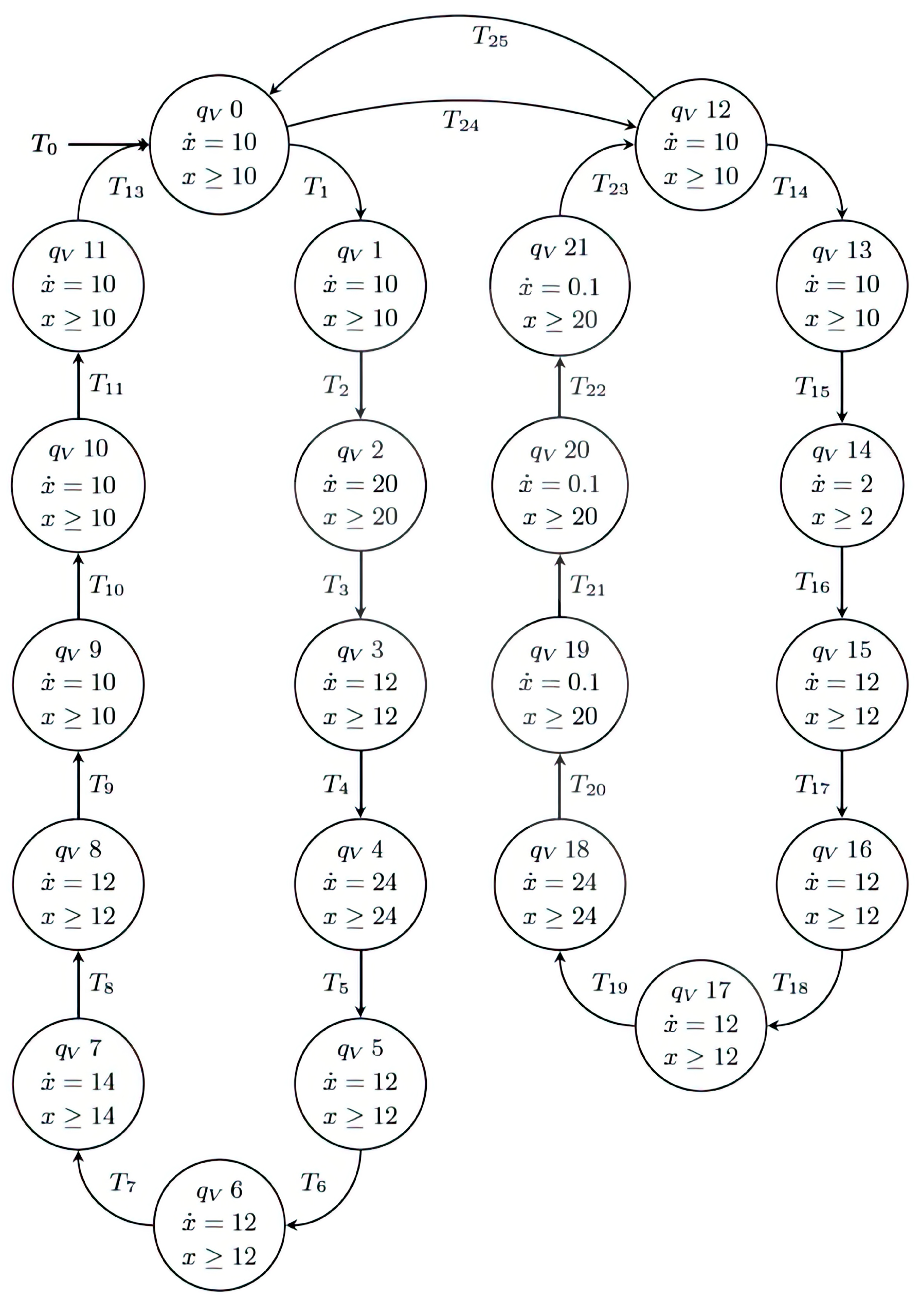
3.4. Digital Hybrid Warehouse Operation Model

Cyber–physical systems are characterized by having a knowledge base in a virtual environment; therefore, to verify that the system is working in its optimal mode, the automata shown in the previous section are modeled with virtual variables, as shown in Figure 4.

3.5. Complex Network of Automated Warehouse

A complex network from an automatic warehouse model is presented. The elements of the storage system that are considered to perform the construction of the complex network are transducers and actuators such as buttons, contactors, motors, and PLCs, and are considered as nodes (Figure 7). The links are interpreted as the relationships between the elements and represent the electrical connection between the nodes of the network (

Table 2. Input and Output Denomination.

Input	Denomination	Output	Denomination	Input	Denomination	Output	Denomination
I10.0	Start button L	Q10.0	Start (Light)	I11.0	Sensor mov X	Q11.0	Forks right
I10.1	Stop Button L	Q10.1	Start L (Light)	I11.1	Sensor mov Z	Q11.1	Forks left
I10.2	Reset button L	Q10.2	Stop L (Light)	I11.2	Emergency stop	Q11.2	Forks Up
I10.3	Sensor conveyor 1L	Q10.3	Stop (Light)	I11.3	Start button D	Q11.3	Start D (Light)
I10.4	Sensor conveyor 2L	Q10.4	Reset L (Light)	I11.4	Stop button D	Q11.4	Stop D (Light)
I10.5	Sensor forks right	Q10.5	Reset (Light)	I11.5	Reset button D	Q11.5	Reset D (Light)
I10.6	Sensor forks middle	Q10.6	Conveyor 1L	I11.6	Sensor conveyor 1D	Q11.6	Conveyor 1D
I10.7	Sensor forks left	Q10.7	Conveyor 2L	I11.7	Sensor conveyor 2D	Q11.7	Conveyor 2D
				I12.0	Sensor current	QW30	Target position

shows assignments of input and output ports).

Construction of Adjacency Matrix

The network constructed from the physical system (Figure 7) is characterized because it is directed, and the adjacency matrix can be constructed. In this matrix, a number “1” is placed for each node that has a link directed to another node. Because there are nodes that are not connected to each other, only the rows of the adjacency matrix that have information on the connections are shown; the interpretation of node/row “I2.0” is that for each activated output (yellow raw), the current consumed will be measured and based on the current value, and the state of the hybrid automata creates an equivalence of the activated outputs and is sent to the pcl/row (blue) in Figure 8.

From the adjacency matrix (see complete matrix in Appendix A), it is observed that, because the network is of the directed type, only the rows of I2.0 and PLC will change, providing there is information to determine the optimal functioning of the system.

3.6. Data Models and Equations

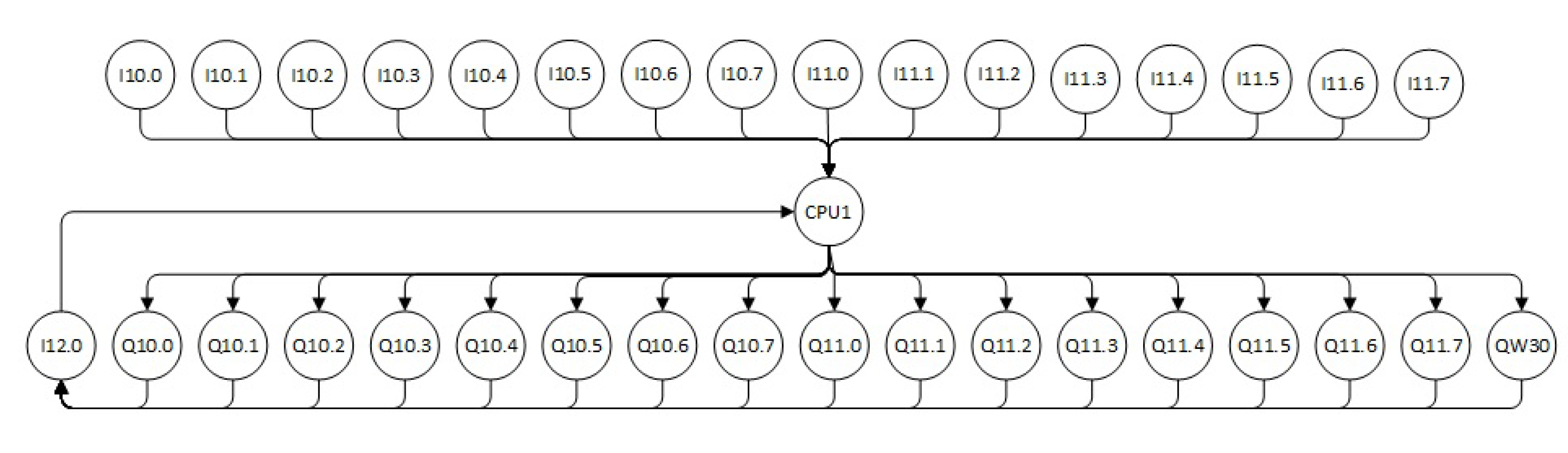
3.6.1. Digital Data Model

The model of the system is based on the monitoring and comparison of the data obtained from the behavior of the physical system and the data obtained from the ideal behavior of the virtual system. The adjacency matrix is composed of rows of data representing information from the sensors and actuators; therefore, the same information can be represented with a set of vectors. For physical inputs, an array of physical binary inputs $D{I}_{P{S}_k}$ is defined, where each place represents the value of different sensors $Sp$ with corresponding physical PLC addresses. The virtual environment simulates the behavior of the physical system, and there is a corresponding array $D{I}_{V{S}_k}$ of the virtual binary with inputs for simulated sensors $Sv$, as shown below:

$$\begin{array}{cc}\hfill D{I}_{P{S}_k}=& [S{p}_{I0.0},S{p}_{I0.1},S{p}_{I0.2},S{p}_{I0.3},S{p}_{I0.4},S{p}_{I0.5},S{p}_{I0.6},S{p}_{I0.7},\hfill \\ \hfill & S{p}_{I1.0},S{p}_{I1.1},S{p}_{I1.2},S{p}_{I1.3},S{p}_{I1.4},S{p}_{I1.5},S{p}_{I1.6},S{p}_{I1.7}]\hfill \end{array}$$

(1)

$$\begin{array}{cc}\hfill D{I}_{V{S}_k}=& [S{v}_{I0.0},S{v}_{I0.1},S{v}_{I0.2},S{v}_{I0.3},S{v}_{I0.4},S{v}_{I0.5},S{v}_{I0.6},S{v}_{I0.7},\hfill \\ \hfill & S{v}_{I1.0},S{v}_{I1.1},S{v}_{I1.2},S{v}_{I1.3},S{v}_{I1.4},S{v}_{I1.5},S{v}_{I1.6},S{v}_{I1.7}]\hfill \end{array}$$

(2)

As can be observed in the adjacency matrix (Appendix A), only one column (strong blue) provides information on the actuators that have been activated by showing a value of “1” when the controller has activated them. The algorithms holds the information of activated outputs by means of a row arrangement (gray row). This arrangement of output elements can be represented as a vector. For the physical output, an array of physical binary outputs $D{O}_{P{S}_k}$ is defined, where each place represents the value of different output $Op$ with corresponding physical PLC addresses. For the virtual system, there is a corresponding array $D{O}_{V{S}_k}$ of virtual binary outputs for simulated outputs $Ov$, as follows:

$$\begin{array}{cc}\hfill D{O}_{P{S}_k}=& [O{p}_{Q0.0},O{p}_{Q0.1},O{p}_{Q0.2},O{p}_{Q0.3},O{p}_{Q0.4},O{p}_{Q0.5},O{p}_{Q0.6},O{p}_{Q0.7},\hfill \\ \hfill & O{p}_{Q1.0},O{p}_{Q1.1},O{p}_{Q1.2},O{p}_{Q1.3},O{p}_{Q1.4},O{p}_{Q1.5},O{p}_{Q1.6},O{p}_{Q1.7},O{p}_{Qw0}]\hfill \end{array}$$

(3)

$$\begin{array}{cc}\hfill D{O}_{V{S}_k}=& [O{v}_{Q0.0},O{v}_{Q0.1},O{v}_{Q0.2},O{v}_{Q0.3},O{v}_{Q0.4},O{v}_{Q0.5},O{v}_{Q0.6},O{v}_{Q0.7},\hfill \\ \hfill & O{v}_{Q1.0},O{v}_{Q1.1},O{v}_{Q1.2},O{v}_{Q1.3},O{v}_{Q1.4},O{v}_{Q1.5},O{v}_{Q1.6},O{v}_{Q1.7},O{v}_{Qw0}]\hfill \end{array}$$

(4)

3.6.2. Analog Data Model

The model also considers vectors for holding data from analog input and outputs connected to physical sensors and actuators. The value of the current consumed by each sensor or actuator is shown. Therefore, the vectors $A{I}_{P{S}_k}$ and $A{I}_{V{S}_k}$ represent the values of analog physical inputs $A{I}_P$ and analog virtual inputs $A{I}_V$, as follows:

$$\begin{array}{cc}\hfill A{I}_{P{S}_k}=& [AI{p}_{I0.0},AI{p}_{I0.1},AI{p}_{I0.2},AI{p}_{I0.3},AI{p}_{I0.4},AI{p}_{I0.5},AI{p}_{I0.6},AI{p}_{I0.7},AI{p}_{I2.0},\hfill \\ \hfill & AI{p}_{I1.0},AI{p}_{I1.0},AI{p}_{I1.0},AI{p}_{I1.0},AI{p}_{I1.0},AI{p}_{I1.0},AI{p}_{I1.0},AI{p}_{I1.0},AI{p}_{I2.0}]\hfill \end{array}$$

(5)

$$\begin{array}{cc}\hfill A{I}_{V{S}_k}=& [AI{v}_{I0.0},AI{v}_{I0.1},AI{v}_{I0.2},AI{v}_{I0.3},AI{v}_{I0.4},AI{v}_{I0.5},AI{v}_{I0.6},AI{v}_{I0.7}AI{v}_{I2.0},\hfill \\ \hfill & AI{v}_{I1.0},AI{v}_{I1.0},AI{v}_{I1.0},AI{v}_{I1.0},AI{v}_{I1.0},AI{v}_{I1.0},AI{v}_{I1.0},AI{v}_{I1.0},AI{v}_{I2.0}]\hfill \end{array}$$

(6)

The function of the sensor I2.0 is to provide a measurement of the current consumed by all the activated actuators.

The $A{O}_{P{S}_k}$ and $A{O}_{V{S}_k}$ represent the vectors of analog physical outputs $A{O}_P$ and analog virtual outputs $A{O}_P$, as follows:

$$\begin{array}{cc}\hfill A{O}_{P{S}_k}=& [AO{p}_{Q0.0},AO{p}_{Q0.1},AO{p}_{Q0.2},AO{p}_{Q0.3},AO{p}_{Q0.4},AO{p}_{Q0.5},AO{p}_{Q0.6},AO{p}_{Q0.7},\hfill \\ \hfill & AO{p}_{Q1.0},AO{p}_{Q1.1},AO{p}_{Q1.2},AO{p}_{Q1.3},AO{p}_{Q1.4},AO{p}_{Q1.5},AO{p}_{Q1.6},AO{p}_{Q1.7},\hfill \\ \hfill & AO{p}_{QW30}]\hfill \end{array}$$

(7)

$$\begin{array}{cc}\hfill A{O}_{V{S}_k}=& [AO{v}_{Q0.0},AO{v}_{Q0.1},AO{v}_{Q0.2},AO{v}_{Q0.3},AO{v}_{Q0.4},AO{v}_{Q0.5},AO{v}_{Q0.6},AO{v}_{Q0.7},\hfill \\ \hfill & AO{v}_{Q1.0},AO{v}_{Q1.1},AO{v}_{Q1.2},AO{v}_{Q1.3},AO{v}_{Q1.4},AO{v}_{Q1.5},AO{v}_{Q1.6},AO{v}_{Q1.7},\hfill \\ \hfill & AO{v}_{QW30}]\hfill \end{array}$$

(8)

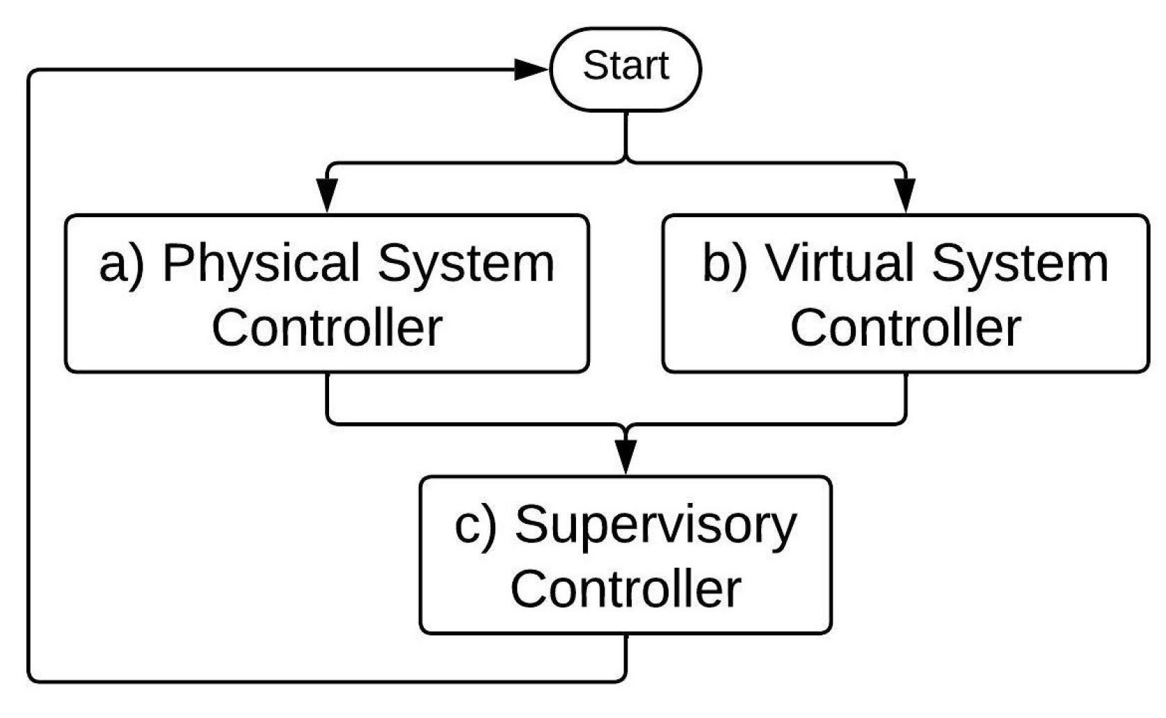
3.7. Development of the System

In the cyber–physical system, the proposed supervisory controller will make decisions based on the comparison of the operation of the physical and the virtual systems (Figure 9).

3.7.1. Physical System Development

This section explains, with a mathematical algorithm, the operation of the physical system (Figure 9a) with its digital variables, $D{I}_{P{S}_k}$ and $D{O}_{P{S}_k}$, and analog variables, $A{I}_{P{S}_k}$ and $A{O}_{P{S}_k}$.

The operation of Algorithm 1, for the physical system, assigns values to the digital and analog input vectors (Equations (9) and (13)) as well as to the output vectors (Equations (11) and (14)). If there is a change of state $S{t}_{P{S}_k}$ in the physical system, the inputs and outputs are measured and assigned correspondingly to the digital input-output and analog input-output vectors. Within the digital analysis, the difference between the current state and the previous state is calculated with Equation (9) for digital inputs $DI{d}_{P{S}_k}$ and Equation (11) for digital outputs $DO{d}_{P{S}_k}$. The input and output differences are stored in their respective memory equations, $DI{m}_{P{S}_k}$ (Equation (10)) or $DO{m}_{P{S}_k}$ (Equation (12)). Regarding the analog analysis, it consists of filtering $(1-\alpha )$ the input and output currents and storing their values in an analog input memory, $AI{m}_{P{S}_k}$, given by (Equation (13)), and an analog output memory, $AO{m}_{P{S}_k}$, according to (Equation (14)), respectively.

Algorithm 1: Development of the digital and analog physical system:

3.7.2. Virtual System Development

This section explains, with a mathematical algorithm, the operation of the virtual system, with its digital variables $D{I}_{V{S}_k}$ and $D{O}_{V{S}_k}$, and analog variables $A{I}_{V{S}_k}$ and $A{O}_{V{S}_k}$ representing the function (Figure 9b) in the following:

Algorithm 2, for the virtual system, is similar to the algorithm of the physical system, except that, in this case, the ideal numerical simulation of the system is carried out, which will help to corroborate the optimal functioning of the physical system. Values are assigned to the vectors of the digital virtual input and digital virtual output $D{I}_{V{S}_k}$ and $D{O}_{V{S}_k}$. In turn, the virtual input and analog virtual output vectors are assigned $A{I}_{V{S}_k}$ and $A{O}_{V{S}_k}$. Unlike Algorithm 1, the signal that was activated in the physical system is expected to start the ideal virtual model, by $S{T}_{P{S}_k}$, to replicate the event in the virtual system, based on the virtual hybrid automaton (Figure 4). The virtual digital and analog values from inputs and outputs are added. An analysis of the previous virtual state and the current digital virtual state is performed with Equation (15) for $DI{d}_{V{S}_k}$ and Equation (17) for $DO{d}_{V{S}_k}$. These input and output differences are assigned to $DImVSk$ by (16) and $DOmVSk$ by (18), respectively. The analogous ideal simulation produces the input and output vectors $AI{m}_{V{S}_k}$ and $AO{m}_{V{S}_k}$, which are filtered by $\alpha$ and $(1-\alpha )$ to produce mean values stored in (19) and (20), respectively, for the analysis of the supervisory controller.

Algorithm 2: Development of the digital and analog virtual system:

3.7.3. Digital Control Operation and Fault Diagnosis

To diagnose faults, the physical input and output memory vectors and the virtual input and output vectors are continuously compared (Figure 9c, but with a synchronization time, considering the change of state in both the physical automata and the virtual automata, and it is implemented Algorithm 3.

Algorithm 3: Development of the digital control

4. Results and Discussion

The presented approach of a cyber–physical system at a supervisory control level is intended for the monitoring and diagnosis of hardware and software failures in an automated storage and retrieval system, as shown in Figure 5. The virtual system is implemented by a real-time numerical simulation to model the behavior of the physical system. Hybrid automata are used to design the control functions of the physical controller and to ease the implementation of the virtual controller. The sensors and actuators were defined as complex network nodes, and their asynchronous activation was defined as events affecting the weight links. The complex network and the hybrid automata for both the digital twin and the physical system were coordinated. Every time that the physical controller activates an actuator or reads a sensor, data vectors save the information and are compared with the corresponding data vectors in the virtual controller. To detect failures in the hardware components, adjacency matrices are compared, and to detect failure in the execution of the sequential logic, the current states are compared. The simulation and implementation of the system present a problem of synchronization between the physical and virtual systems. This problem was solved by considering a time of delay between the data transfer and the change in the physical state and virtual state.

Figure 9 shows the execution of the physical system and the virtual system. It can be observed that the virtual and physical hybrid automata change at the same time with an specific time of synchronization. In Figure 10, input and output changes can also be observed, besides changes between 0 and 1. The system updates and saves the values from the activation and deactivation events, and the algorithms detect discrepancies of data values of the physical controller with respect to data values of the virtual system. In this way, it is possible to detect failures in sensors, actuators, and in the execution of the control logic.

To corroborate the operation of the algorithm, the stored information presented in the Figure 9 was examined. In the case where there are no failures, the data vectors are identical, and in the case that the data are not equal, there are failures. Figure 11 shows the difference in the data vectors with red rectangles to indicate failures and the green rectangles to indicate that the elements are working correctly.

Finally, Figure 12 shows an operator panel with indicators to display the elements that present a failure.

In order to evaluate the efficiency of the system, four different cases (row represents the number of simulations) of failure diagnosis were evaluated in different stages of the process, and the tests were carried out both in the loading and unloading configuration of the warehouse. It is observed that the system is capable of diagnosing and locating the failures induced in inputs and outputs selected in

Table 3. Input and Output Denomination.

No. Simulation	State	Input/Output Induce Fault	Input Physical Vector	Input Virtual Vector	Output Physical Vector	Output Virtual Vector	Fault Detection
1	$q_{P3}$	I10.4, Q11.4	I10.4 = 0	I10.4 = 1	Q11.4 = 0	Q11.4 = 1	I10.4, Q11.4—Correct
2	$q_{P9}$	I10.5, Q11.0	I10.5 = 0	I10.5 = 1	Q11.0 = 0	Q11.0 = 1	I10.5, Q11.0—Correct
3	$q_{P14}$	I11.0, I11.1, Q11.4	I11.0 = 0, I11.1 = 0	I11.0 = 1, I11.1 = 1	Q11.4 = 0	Q11.4 = 1	I11.0, I11.1, Q11.4—Correct
4	$q_{P19}$	I10.5, Q11.6, Q11.7	I10.5 = 0	I10.5 = 1	Q11.6 = 0, Q11.7 = 0	Q11.6 = 1, Q11.7 = 1	I10.5, Q11.6, Q11.7—Correct

; in the third column, a specific number of induced failures is selected, and it is observed that the system in the eighth column can satisfactorily diagnose and locate all the induced failures.

The proposed approach for a basic cyber–physical system is composed of a virtual twin simulating the process of the physical system. The virtual twin executed simultaneously with the operation of the physical systems allows for a comparison in real time. When the behavior of both do not match, a fault is diagnosed. The presented approach can be extended to diverse manufacturing systems.

5. Conclusions

This work proposed a novel scheme of a basic cyber–physical system that incorporates a virtual system at the supervisory control level. The virtual system is executed in a real-time simulation, providing means to monitor and diagnose failures in sensors, actuators and in the execution of the sequential logic control. In this approach, the digital twin is mainly a numerical simulation of the process and its controller, which is made up of algorithms that combine a hybrid automata as a virtual controller, along with the sensors and actuators modeled in a complex network. The implemented system acts as a supervisory control system capable of diagnosing and locating failures in physical systems in real time. The algorithms were validated in an automated storage and retrieval system. The implementation was required to solve some synchronization problems presented in the coordination of the digital twin with the physical system. One of the main tests showed that the system was capable of detecting and locating failures in two actuators and two sensors. The obtained results validate that the proposed scheme is able to diagnose and locate concurrent faults in real time and can be incorporated as an advance automation function of manufacturing systems.

References

1. TcaciucGherasim, S.A. A Solution for an Industrial Automation and SCADA System. In Proceedings of the 2022 International Conference and Exposition on Electrical And Power Engineering (EPE), Iaşi, Romania, 20–22 October 2022; IEEE: Piscataway, NJ, USA, 2022; pp. 297–300. [Google Scholar]
2. Khadra, A.; Rammal, R. SCADA System for Solar Backup Power System Automation. In Proceedings of the 2022 International Conference on Smart Systems and Power Management (IC2SPM), Beirut, Lebanon, 10–12 November 2022; IEEE: Piscataway, NJ, USA, 2022; pp. 75–79. [Google Scholar]
3. Nuhel, A.K.; Sazid, M.M.; Ahmed, K.; Bhuiyan, M.N.M.; Hassan, M.Y.B. A PI Controller-based Water Supplying and Priority Based SCADA System for Industrial Automation using PLC-HMI Scheme. In Proceedings of the 2022 IEEE International Conference on Artificial Intelligence in Engineering and Technology (IICAIET), Kinabalu, Malaysia, 13–15 September 2022; IEEE: Piscataway, NJ, USA, 2022; pp. 1–6. [Google Scholar]
4. Hamzah, M.; Islam, M.M.; Hassan, S.; Akhtar, M.N.; Ferdous, M.J.; Jasser, M.B.; Mohamed, A.W. Distributed Control of Cyber Physical System on Various Domains: A Critical Review. Systems 2023, 11, 208. [Google Scholar] [CrossRef]
5. Zhang, K.; Shi, Y.; Karnouskos, S.; Sauter, T.; Fang, H.; Colombo, A.W. Advancements in industrial cyber-physical systems: An overview and perspectives. IEEE Trans. Ind. Inform. 2022, 19, 716–729. [Google Scholar] [CrossRef]
6. Villalonga, A.; Beruvides, G.; Castano, F.; Haber, R.E. Cloud-based industrial cyber–physical system for data-driven reasoning: A review and use case on an industry 4.0 pilot line. IEEE Trans. Ind. Inform. 2020, 16, 5975–5984. [Google Scholar] [CrossRef]
7. Alshalalfah, A.L.; Mohamed, O.A.; Ouchani, S. A framework for modeling and analyzing cyber-physical systems using statistical model checking. Internet Things 2023, 22, 100732. [Google Scholar] [CrossRef]
8. Li, P.; Zhang, F.; Yang, Y.; Ma, X.; Yao, S.; Yang, P.; Zhao, Z.; Lai, C.S.; Lai, L.L. The integrated modeling of microgrid cyber physical system based on hybrid automaton. Front. Energy Res. 2022, 10, 748828. [Google Scholar] [CrossRef]
9. Staroletov, S. Automatic proving of stability of the cyber-physical systems in the sense of Lyapunov with KeYmaera. In Proceedings of the 2021 28th Conference of Open Innovations Association (FRUCT), Moscow, Russia, 25–29 January 2021; IEEE: Piscataway, NJ, USA, 2021; pp. 431–438. [Google Scholar]
10. Ravasio, D.; Tuissi, L.; Spinelli, S.; Ballarino, A. A Compressed Air Network Energy-Efficient Hierarchical Unit Commitment and Control. In Proceedings of the 2023 15th International Conference on Computer and Automation Engineering (ICCAE), Sydney, Australia, 3–5 March 2023; IEEE: Piscataway, NJ, USA, 2023; pp. 469–473. [Google Scholar]
11. Guo, Z.; Zhang, Y.; Zhao, X.; Song, X. CPS-based self-adaptive collaborative control for smart production-logistics systems. IEEE Trans. Cybern. 2020, 51, 188–198. [Google Scholar] [CrossRef] [PubMed]
12. Sun, T.; Xia, W.; Zhao, X.; Sun, X.M. A Novel Mathematical Characterization for Switched Linear Systems Based on Automata and Its Stabilizability Analysis. IEEE Trans. Control. Netw. Syst. 2023. [Google Scholar] [CrossRef]
13. Alonso, M.; Turanzas, J.; Amaris, H.; Ledo, A.T. Cyber-physical vulnerability assessment in smart grids based on multilayer complex networks. Sensors 2021, 21, 5826. [Google Scholar] [CrossRef] [PubMed]
14. Zhao, Z.; Xu, Y.; Li, Y.; Zhao, Y.; Wang, B.; Wen, G. Sparse actuator attack detection and identification: A data-driven approach. IEEE Trans. Cybern. 2023, 53, 4054–4064. [Google Scholar] [CrossRef] [PubMed]
15. Pósfai, M.; Barabasi, A.L. Network Science; Citeseer: London, UK, 2016. [Google Scholar]
16. Giudici, R. Introducción a la Teoría de Grafos; Equinoccio: Baruta, Miranda, Venezuela, 1997. [Google Scholar]
17. Mu, D.; Yue, X.; Ren, H. Robustness of Cyber-Physical Supply Networks in Cascading Failures. Entropy 2021, 23, 769. [Google Scholar] [CrossRef] [PubMed]
18. Platzer, A. Logical Foundations of Cyber-Physical Systems; Springer: Cham, Switzerland, 2018; Volume 662. [Google Scholar]
19. Lin, H.; Antsaklis, P.J. Hybrid Dynamical Systems; Foundations and Trends® in Systems and Control: Delft, The Netherlands, 2015. [Google Scholar]
20. Meyn, S. Control Techniques for Complex Networks; Cambridge University Press: Cambridge, UK, 2008. [Google Scholar]
Figure 1. (a) Undirected network. (b) Directed network.
Applsci 13 10603 g001
Figure 2. Proposed scheme of the cyber–physical system.
Applsci 13 10603 g002
Figure 3. Physic hybrid automaton.
Applsci 13 10603 g003
Figure 4. Virtual hybrid automaton.
Applsci 13 10603 g004
Figure 5. Automatic warehouse.
Applsci 13 10603 g005
Figure 6. (A) Sensors and actuators in conveyor belt download. (B) Sensors and actuators in conveyor belt load. (C) Sensors and actuators in elevator base.
Applsci 13 10603 g006
Figure 7. Complex network of the physical system.
Applsci 13 10603 g007
Figure 8. Adjacency Matrix.
Applsci 13 10603 g008
Figure 9. (a) Physical System Controller; (b) Virtual System Controller; (c) Supervisory Controller.
Applsci 13 10603 g009
Figure 10. Development of the cyber–physical system.
Applsci 13 10603 g010
Figure 11. Diagnosis of faults.
Applsci 13 10603 g011
Figure 12. Location of faults.
Applsci 13 10603 g012