Article

Explicit Method in the Seismic Assessment of Unreinforced Masonry Buildings through Plane Stress Elements

Department of Civil Engineering, Institute for Sustainability and Innovation in Structural Engineering (ISISE), Advanced Production and Intelligent Systems (ARISE) Associated Laboratory, University of Minho, 4800-058 Guimaraes, Portugal
*
Author to whom correspondence should be addressed.
Appl. Sci. 2023, 13(19), 10602; https://doi.org/10.3390/app131910602
Submission received: 14 August 2023 / Revised: 14 September 2023 / Accepted: 18 September 2023 / Published: 22 September 2023
(This article belongs to the Special Issue Seismic Assessment and Design of Structures: Volume 2)

Abstract

:
The complex nonlinear behaviour of unreinforced masonry (URM), along with the interaction between structural elements, still represents a challenge for the seismic assessment of existing URM buildings. A large variety of mathematical tools have been developed in the last decades to address the issue. The numerical work herein presented attempts to provide some insights into the use of FEM models to obtain reliable results from nonlinear dynamic analyses conducted with explicit methods. Through plane stress elements, two in-plane mechanisms were studied to identify optimal parameters for unreinforced masonry elements subjected to dynamic actions. The results were then compared with outcomes generated by an implicit solver. Subsequently, these parameters were used in nonlinear dynamic analyses on a building section for the seismic assessment in both unreinforced and reinforced conditions. The element type, hourglass control, damping, and bulk viscosity influence the dynamic response, mainly when the nonlinearities become larger. The hourglass control techniques employ a scaling factor to suppress the occurrence of spurious modes. Values ranging from 0.01 to 0.03 have shown effective results. When the stiffness-damping parameter for Rayleigh damping is of a similar order of magnitude or lower than the time increment without damping, the time increment remained in feasible ranges for performing analysis. Additionally, the bulk viscosity can stabilise the response without causing substantial alterations to the time increment if the values are under 1.00.

1. Introduction

Masonry is a widespread material that has been employed for centuries in various types of structures around the world, ranging from monuments and historical construction to ordinary buildings like houses, many of them settled in earthquake-prone areas. Unreinforced masonry (URM) buildings, while capable of withstanding gravitational loads, are highly vulnerable to horizontal dynamic loads. Therefore, existing URM buildings, including historical buildings and monuments, are susceptible to damage involving cracks or the partial or total collapse of the structure, even under moderate ground motion. Masonry is a composite material made of units and joints. Units comprise a wide range of materials, such as natural stones, bricks, adobe, and others. Joints can be dry or made of cement-, lime-, or mud-based mortar.
The poor performance of unreinforced masonry under lateral loads, particularly seismic excitations, arises from the low tensile and shear strength of the material. The damage of masonry during earthquakes are normally classified into two types: in-plane failure and out-of-plane failure. The three basic in-plane (IP) damage patterns are flexural failure, shear-diagonal failure, and shear sliding (see Figure 1). This type of response is more ductile [1]. Geometry, boundaries, loading conditions, and mechanical properties govern the load capacity and failure mode. On the other hand, openings affect the IP behaviour creating points of weakness [2].
In the case of out-of-plane (OOP) damage, vertical, horizontal, or diagonal (or a combination of) flexural cracks develop, resulting in partial or complete collapse [3], as shown in Figure 1. This type of damage is fragile, being the first collapse mechanism and more frequent in existing URM buildings when no prevention is taken [4]. OOP mechanisms require less energy compared to IP mechanisms for activation. This implies that even a small seismic action can induce OOP damage or even lead to collapses [5,6]. Consequently, OOP mechanisms have a higher risk for both the stability of the building and human life. OOP mechanisms are more likely to occur when there are weak connections with other structural elements, such as transversal walls, floors, and roofs. Moreover, flexible floors and roofs can contribute to the collapse of walls in the OOP direction. The geometrical layout (in elevation and horizontal plane) of the building and load conditions play a key role [7,8].
Figure 1. IP failure modes (adapted from [9]): (a) flexural failure; (b) shear-diagonal failure; (c) shear-sliding failure. Examples of OOP failure modes (adapted from [10]): (d) mechanism in long walls; (e) mechanism in short walls; (f) mechanism of the corner; (g) mechanism of the tympanum (gable).
Applsci 13 10602 g001
Over time, builders in earthquake-prone areas have implemented empirical strengthening techniques by trial and error to enhance the performance of URM structures, such as ties, buttresses, and timber skeletons [10]. However, it is in recent decades that the scientific community has begun to systematically study these techniques with a scientific approach. Additionally, advancements in technology have enabled researchers and builders to develop methods using contemporary materials. A brief review of the main strengthening techniques is presented in Section 2.
The accurate prediction and assessment of the damage evolution in existing URM buildings under seismic actions remain challenging tasks due to the complexity of the material and the interaction between all the structural elements, along with the nature of the earthquakes [11]. Researchers have developed a wide variety of mathematical models and strategies for this type of structure, aiming to provide more efficient procedures while ensuring reliable results [12]. The selection of mechanical properties depends on the chosen modelling strategy and applied analysis method [13]. Section 3 presents an overview of different modelling strategies and types of analyses, as well as time integration methods used to solve the system of equations, i.e., implicit and explicit solvers. For the sake of brevity, the most important features of these methods are highlighted, while mathematical formulations are not described.
The comparison between implicit and explicit methods in FEM modelling has been explored in several fields including metal forming, impact, and contact problems. In the case of masonry structures, explicit methods have been applied to study the effects of blast loadings on both unreinforced and reinforced conditions [14]. Pereira and Lourenço [15] used a FEM model with an explicit solver to study explosions in a historical masonry building. A similar approach was carried out by Tse et al. [16] to evaluate the response of a historical structure built with earthen masonry to blast loads. Nevertheless, the studies and applications of explicit methods for the seismic assessment of URM buildings are scarce. Tarque et al. [17] created a FEM model using shell elements of a house made of adobe, simulating the results from an experimental campaign conducted on a shake table test. Yang [18] developed a FEM model of a URM building using DIANA FEA 10.3 software to compare the results of implicit and explicit methods. The nonlinear dynamic analyses demonstrated that both approaches yielded similar responses. Finally, Noor-E-Khuda [19] studied the OOP behaviour of masonry walls employing shell elements, exploring variations in openings and boundary conditions. The FEM model was then subjected to a lateral incremental load (nonlinear pushover analysis).
FEM modelling requires meticulous consideration, including the selection of suitable elements for the specific problem at hand. For example, linear elements that are fully integrated can exhibit shear locking, while linear elements with reduced integration are susceptible to hourglass distortions (Section 6). In the FEM modelling of URM buildings, particularly in explicit solutions, critical aspects such as shear locking, hourglass effects, and hourglass control techniques, among others, have not been addressed in prior works. Therefore, the present study aims to provide some insights into the application of explicit methods in 2D FEM modelling. Its primary objective was to conduct a comparative study between implicit and explicit methods, specifically addressing in-plane behaviour to simulate two frequent failure types observed in masonry walls under seismic loading. This can provide the users with a practical understanding of the effect of each parameter used in an explicit method, specifically in Abaqus/Explicit.
Four models were generated to perform a parametric analysis. Two of these models focused on reproducing IP behaviour, targeting shear-diagonal failure and flexural failure, using 2D FEM elements, particularly plane stress elements. This type of element is related to states where the stress component normal to the element plane is negligible. Although masonry can undergo triaxial stress, plane stress elements are frequently used to simulate structural elements with small thickness where the loads act in the plane, such as masonry walls [20,21,22].
The other two models represent a section of a URM building (employing 1D and 2D FEM elements). The geometrical characteristics of the models are detailed in Section 4. The concrete damage plasticity model is adopted to account for the nonlinear properties of the masonry (Section 5). A key objective of this work was to compare the simulations conducted for masonry piers using both implicit and explicit methods with the Abaqus/CAE 2019 software [23]. The influence on the results of the element types used for modelling the structural problem, along with other parameters (discussed in Section 6), was considered. Initially, the IP mechanisms allowed the assessment of the performance of each parameter used in the explicit solver. Subsequently, through the explicit method, the parameters that exhibited better performance were used in the seismic assessment of the building section, considering both the unreinforced and reinforced conditions (Section 7).

2. Strengthening Techniques

The strengthening techniques for existing URM buildings can be classified into three categories [3]. The first group focuses on local interventions to improve the tensile and shear capacity of the most vulnerable elements. The second category aims to enhance the global response by inducing the so-called “box behaviour”, where all the structural elements are tied together to act as a single body. Finally, the most recently applied techniques target the reduction of seismic demand through base isolation and enhancement of energy dissipation using dampers [3]. It is common to employ a combination of techniques in the strengthening interventions.

2.1. Local Strengthening

Due to the masonry’s limited tensile and shear strength, most techniques address this issue by adding specific types of reinforcements on the external surfaces of the walls or within the interior. This reinforcement is capable of withstanding tensile stresses, delaying the occurrence of cracks, restricting their propagation, and increasing the deformation capacity of the material [3].
When a wall loses its mortar and contains voids, the most common repair method is the repointing and injection of a fluid with some type of binder agent, such as cement- or lime-based grouts [3,24,25]. It is important to note that compatibility must be considered, since this is an irreversible intervention [25]. the presence of multi-leaf (two or three leaves) walls in historical buildings is frequent. If the leaves are weakly connected, the carrying capacity of the wall under lateral and axial forces decreases. The strengthening of these walls is carried out using grout injection or introducing transversal metallic bars (sometimes post-tensioned) or fibres to connect the leaves [3,24,25,26,27,28].
Applying a reinforcing layer to the surfaces is another frequently employed technique. One of the typical reinforcements comprises a steel mesh embedded in mortar or concrete [3,24,29]. This technique increases the IP and OOP resistance capacity of the element [3]. The mass increment, irreversibility and possible mechanical incompatibilities are considered factors when applying concrete layers.
In recent years, fibre-based materials have gained popularity as a reinforcement applied to surfaces given their high tensile strength [3,30]. The most frequent fibres are made from a variety of materials, including carbon, glass, basalt, aramid, polymers, and even natural fibres [3,31]. Two primary systems are commonly used for reinforcement. Fibre-reinforced polymers (FRP) are fibre sheets or strips where the fibres are embedded in a resin matrix, which are then bonded to masonry using an epoxy binder [3]. In textile-reinforced mortar TRM, fibres are arranged to form a mesh that is applied to masonry with cement- or lime-based mortar [3,30]. These systems significantly improve the OOP and IP response of these structural elements [3,30,32,33,34].
Internal reinforcement serves as an alternative when surface interventions are not permitted due to concerns about their impact on the structure’s aesthetics [3]. This technique involves drilling vertical holes along the height of the wall to introduce steel bars. The bars can act as passive elements or be post-tensioned (active elements) [35]. If properly executed, the wall can resist both IP and OOP actions [3].

2.2. Global Strengthening

The primary weakness of existing masonry buildings lies in the lack of effective connections among their structural elements, causing the OOP overturning of facades and parapets [7]. In general, the solution is to tie all the elements together, ensuring that the inertia forces are uniformly transferred and distributed throughout the entire structure. Techniques to achieve this behaviour include the construction of RC elements, stiffening of floors and roofs with rigid connections to walls, and the incorporation of ties and timber elements [3,36].
The construction of RC collar beams at floor/roof levels can induce box behaviour. A complete confining effect is achieved if RC columns are also built in intersections and midspan of walls [3]. However, this procedure is also complicated to apply and invasive [3]. Timber and steel are also used to build collar beams on top of the walls, which are reversible and less invasive [10,24,37]. An alternative is to transform flexible floors and roofs into stiff diaphragms, which can be used in conjunction with collar beams (RC or timber) [3,24]. Stiffening methods involve, among others, the addition of wooden planks or sheathing, horizontal diagonal bracing made of metallic elements or FRP strips, RC layers, and even the complete substitution of the floor/roof by a RC slab [7,38,39]. The diaphragm must be properly connected to the surrounding walls to ensure the effective transfer of lateral loads [26]. The reader is referred to [40] for further information regarding connections.
Ties, often made of steel rods, serve as a technique to connect structural elements and restrain their outward motion [3]. They work only under tension and can tie together walls (normally parallel), arches, vaults, and domes [3,10,24]. This technique is considered a reversible intervention and does not considerably increase the mass of the building. They are preferably placed at the levels of floors and roofs, or close to the impost line in arches and vaults. In the case of earth-based structures, ties and collar beams made of timber are more common [10,41]. Ties are one of the most applied strengthening techniques, as they effectively reduce the likelihood of OOP collapses [42]. The reader can refer to Gkournelos et al. [3] and Ortega et al. [10] to extend the knowledge.

2.3. Reduction of the Seismic Demand and Energy Dissipation

The techniques used to reduce the seismic demand and dissipate energy include base isolation and passive energy dissipation devices (PED), also known as dampers. These methods are rarely used in existing URM buildings, although researchers are currently assessing and developing more suitable devices for URM buildings. Among these solutions, base isolation has been the most frequently applied technique to this type of structures [43]. Base isolation aims to decouple the building from the ground to decrease the seismic excitation transmitted to the structure by placing a flexible layer between the foundation and the structure [44,45].
There are five types of PEDs, namely friction, yielding, phase transformation, viscous fluid, and viscoelastic devices. Friction devices dissipate energy when two or more surfaces slide one on top of the other [46]. In yielding devices, the energy is dissipated through the plastic deformation of a metal element and should be changed after a strong earthquake if it is yielded [47]. Special friction and yielding connectors have been developed to fix floors to walls [48], to link planks to each other for timber floors [49], or as a part of the anchoring systems to tie perpendicular walls [50]. Phase transformation devices normally use wires made of shape memory alloys, which also yield but with the capability of recovering the original shape [51]. One end of the device is attached to a rigid roof, while the other end is anchored to the walls. The devices can also be introduced into post-tensioned vertical ties in slender structures such as towers [52]. Viscous fluid (VF) devices dissipate energy when a solid body (usually a piston with holes) moves in a viscous fluid [46]. These devices have been implemented as a connection point between the wall and the steel rod in tie systems [53]. Viscoelastic (VE) devices draw on the shear deformation of viscoelastic layers bonded to steel plates that move one with respect to the other [46]. Nochebuena-Mora et al. [43] furnish detailed information regarding energy dissipation devices for historical constructions.

3. Modelling Strategies

3.1. Modelling Strategies for Material

The modelling adopted depends on the level of accuracy and simplicity. Three strategies are commonly used, namely detailed micro-modelling, simplified micro-modelling, and macro-modelling [12]. In detailed micro-modelling, the real texture of the structural component (wall, arch, vault, etc.) is replicated [11]. Units and mortar are continuous elements, and the interface in between is a discontinuity, representing the plane of failure (Figure 2a). In simplified micro-modelling, units are expanded continuous elements, while the mortar is represented by an interface, which is a discontinuity, and, thus, the line of failure (Figure 2b). In this case, part of the accuracy is lost [12]. However, these two strategies are a time-consuming task when assembling the model and demand a high computational effort, which limits their application to larger scales [11]. In macro-modelling, masonry is considered a deformable homogenous continuum [11]. There is no distinction between units and mortar, which are smeared out in only one body (Figure 2c). This generally reduces the computational effort. Given the complexity of the material, the selection of a suitable constitutive law is challenging [11]. The macro-modelling approach is more suitable for large models such as complete buildings [36].

3.2. Strategies for Numerical Models

The analysis of URM buildings can be performed by adopting four numerical modelling approaches, namely the finite element method (FEM), discrete element method (DEM), rigid macroblocks, and equivalent frame model (Figure 3). A general description is given in the following. Modelling strategies for URM buildings are treated in more detail in [11,54,55,56,57,58,59,60].
In FEM models, the continuous domain is discretized into small and simpler subdomains called elements, which are connected by nodes to form a mesh. These models represent structural problems using various types of elements, such as 1D, 2D, 3D, springs, interfaces, etc. [11]. FEM models are versatile and can solve both static and dynamic problems with linear or non-linear solutions. While implicit methods are commonly used for solving nonlinear problems, explicit solutions can also be applied when needed. Currently, FEM models, combined with a macro-modelling approach, are extensively used for the overall seismic assessment of unreinforced masonry (URM) buildings [36].
DEM is a collection of numerical techniques used to analyse the dynamics of a set of particles or bodies treated as a discontinuous material. In the seismic evaluation of unreinforced masonry (URM) buildings, DEM models typically consist of blocks representing individual units or larger portions of the structure, and their interactions are defined through contact points with specific contact properties [11,36]. These blocks in DEM models can be treated as either rigid or deformable bodies [61]. DEM models employ explicit solutions to address highly nonlinear geometric problems, enabling the simulation of collapse mechanisms with large displacements [36]. For more comprehensive details, refer to Lemos [62].
The equivalent frame method consists of the simplification of the building by identifying its main load-bearing components, such as piers and spandrels. The discretization process becomes a challenging task when the building has a complex geometry where openings are irregularly distributed [11]. Subsequently, these components are typically replaced with nonlinear columns, beams, or blocks, which are connected using rigid nodes, plastic hinges, interfaces, or springs [63]. The formulation captures the shear-diagonal deformation, flexural response, and shear sliding of the components [64]. The global response is only related to the IP behaviour of the walls and floors, and no information is provided regarding the OOP performance [11].
In the last strategy, the building is idealized as a structure composed of rigid macroblocks, which are delimited by the expected collapse mechanisms. These mechanisms can be defined according to the observed damage in similar structures during an earthquake, experimental campaigns, or experience [36]. It is noted that the adopted discretisation dominates the response and can be overestimated if the mechanism with the lowest capacity is neglected. The limit analysis is generally used to evaluate the seismic response.

3.3. Type of Analyses

Numerical models can be used to perform different types of analyses, which are selected based on the desired outputs. The common analyses used in the seismic assessment of buildings include limit analysis, linear static analysis, nonlinear static analysis (pushover analysis), linear dynamic analysis in the time domain, linear dynamic analysis in the frequency domain, and nonlinear dynamic analysis in the time domain (nonlinear time history analysis) [11,36].
Limit analysis implements solutions based on either static or kinematic theorems, requiring minimal input information (geometry and load conditions) and low computational power [11]. Seismic assessment with macroblocks normally employs this analysis type. It provides results on collapse mechanisms and seismic load capacity [36]. All types of linear analyses are inadequate for capturing the dynamic response of URM buildings [11]. Masonry exhibits a high nonlinearity and low tensile strength, making linear analysis unsuitable even for moderate ground motions [36].
Nonlinear static analysis is a very common and standardised analysis to evaluate the seismic capacity of existing URM buildings [11,36]. In this case, seismic action is incrementally applied as a lateral force [36]. The analysis accounts for the nonlinear material properties. The nonlinear differential equations are normally linearised and solved by iterative methods, using, for example, the Newton–Raphson method. Implicit solvers may encounter convergence problems when the response is highly nonlinear. However, this approach offers a suitable balance between accuracy and computational demand since it can find the post-peak behaviour [11].
On the other hand, in nonlinear dynamic analysis, the structure is subjected to time-dependent actions, and the response accounts for the inertia and damping forces [11]. The actions are either recorded earthquakes or artificially generated signals. It is the most advanced and complex type of analysis since it requires time integration methods to solve the differential equations in the time domain [11,36]. Implicit solvers are commonly used in FEM models, while explicit methods are more frequently applied in DEM models [36]. The computational demand for the implicit solvers is high due to the solution of differential equations, nonlinear behaviour, and convergence issues.

3.4. Numerical Solvers: Explicit and Implicit Methods

Time integration methods are numerical techniques developed to approximate the equations of motion using a step-by-step direct integration procedure. Equations (1) and (2) are the linear and nonlinear equations of motion of a discrete structural, respectively [65]:
M U ¨ + C U ˙ + K U = R ( t )
M U ¨ + C U ˙ + N ( U ) = R ( t )
where M is the structural mass matrix, C is the viscous damping matrix, K is the linear stiffness matrix, N is the vector of nonlinear internal forces related to the current vector displacements U at time t , and R ( t ) is the vector of time-dependent external forces. The subscript ( · ) indicates time derivatives of the displacement vector U . The problem consists of finding the time history solution for U = U ( t ) , with the defined initial conditions U ( 0 ) = U o and U ˙ ( 0 ) = U ˙ o , which for seismic actions are equal to zero. Direct numerical integration methods discretise the time t into time intervals Δ t and assume that Equations (1) and (2) are solved for each time interval considering variations in displacements, velocities, and accelerations at each time step. Therefore, the total response is a sequence of independent problems, where the conditions change from one step to another [66]. Depending on the assumptions made about these variations, different integration schemes are derived, which can be further classified into explicit and implicit methods [67].
In the explicit methods, the solution at time t + Δ t is calculated considering the equilibrium conditions at time t , using the known values of U , U ˙ , and U ¨ found in the previous step. The vector displacement (at the end of the time interval) is not a function of the loads or stiffness (at the end of the time step). As a result, no iteration is needed, and the method can directly proceed to the next time interval [66,67]. The approach allows for the incorporation of very complex constitutive laws and does not require the inversion of the stiffness matrix, resulting in a low computational cost per time step. Nevertheless, explicit methods are conditionally stable, meaning that the time increments should be small enough to ensure numerical stability. The time interval depends on the highest frequency of the discrete system without damping [67]. The introduction of damping affects the time step, reducing its length (Section 5). The main explicit solvers include the second-order central difference methods, which are suitable for large-scale models in stress-type analysis, and the fourth-order Runge–Kutta method [67].
In implicit solvers, the solution for displacements at the current increment Δ t requires the velocities and accelerations of the current time itself, so trial values are assumed and refined by an iterative process [66,67]. This implies that the stiffness matrix should be inverted at each time step for the calculation of displacements. Implicit methods are normally unconditionally stable, where the maximum time interval is determined by the desired accuracy [67]. Conversely, the time step may be much larger than in explicit methods, and, thus, fewer intervals are required. The implicit time integration schemes include the Newmark methods, Wilson-θ method, and Houbolt methods [68]. Among these, Newmark methods have better accuracy in structural problems. A generalized form of Newmark methods is the Hilber–Hughes–Taylor (HHT) method. It introduces the parameter α in the original Newmark formulation to improve the stability with larger steps. This approach has no effect on the response of low frequencies, which are of interest in structural problems, while it damps out the spurious highest modes that arise from the discretisation of the system [68]. Due to this improvement, the HHT method is used in most commercial software packages.
For nonlinear problems, either static or dynamic, the internal force vector N ( U ) is a nonlinear function of displacement U , which corresponds to the constitutive law of the material. To find the solution, numerical approaches such as Newton–Raphson methods (regular, modified, and linear) or Quasi-Newton (secant stiffness) method are applied [20,69]. There is extensive literature on these subjects; interested readers are referred to [20,66,67,69,70] as a first approach to nonlinear static and dynamic analyses.

4. Case Studies

4.1. Piers of Gaioleiro Buildings (Portugal)

Two masonry piers of a Portuguese building typology (Gaioleiro buildings) were selected and modelled, aiming to evaluate first the performance of the numerical tools at the structural element level. Gaioleiro buildings, built in Portugal during the late 19th and early 20th centuries, typically consist of four to six levels [26,71]. The interstory height varies between 2.7 and 3.7 m, with the ground floor usually being higher than the other levels. To provide ventilation and light, these buildings have central or lateral shafts (Figure 4). The foundations and façades are built using rubble masonry, while lateral walls are often made of brick [71]. The thickness of the façades ranges from 0.50 to 1.00 m on the ground floor, and reduces as the elevation increases [72]. The inner walls can be made of brick (walls parallel to the façades) or timber planks with plaster (walls perpendicular to the façades). Floors are flexible diaphragms composed of timber joists and timber planks, or metallic profiles and jack arches. Joists and metallic profiles are set perpendicular to the façades with a spacing of 0.35–0.40 m, and are simply supported on the walls. As for the roofs, they are simple timber structures that cannot be considered trusses [71,72].
Figure 4c highlights two specific piers of the façade selected to be subjected to IP dynamic actions, aiming to induce shear-diagonal and flexural failures. Pier 1, which is located on the ground floor, is 1.90 × 1.80 × 0.70 m (length × height × thickness). Due to its geometry and loading condition, shear-diagonal failure is likely to occur in this panel. On the other hand, Pier 2, at the top of the façade, measures 1.55 × 2.55 × 0.45 m. This panel is used to simulate flexural damage since it is slender, and its level of compression is considerably lower than that of Pier 1. For the simulation, equivalent masses were placed on top of the panels to represent the weight of the structural elements they carry. The normal stress applied at the top of Pier 1 and Pier 2 is equal to 328.75 kPa and 21 kPa, respectively. The numerical models were generated in Abaqus [23], using quadrilateral plane stress elements with a characteristic length of 0.05 m. The elements have the real thickness of the piers. The mechanical properties of the masonry are detailed in Section 4.

4.2. Viceregal Dwellings (Mexico)

Figure 5 depicts a typical viceregal dwelling constructed during the 17th and 18th centuries in various cities across Mexico during the Spanish colonial period. The building comprises two floors with interstory heights ranging from 4.95 to 5.10 m. The architectural layout features rooms surrounding two patios, with doors and windows aligned. The wall thicknesses are 0.90 m for the façade, 0.80 m for the inner walls on the ground floor, and 0.60 m for the inner walls on the upper floor [73,74].
Rubble masonry was employed for constructing the foundations and walls, whereas columns and arches were built with dressed stones. The building features flexible flat slabs for both floor and roof, consisting of a large array of timber joists with a cross-section of 0.15 × 0.20 m. These joists are arranged perpendicular to the façade, with a spacing of 0.30 m, providing support for a layer of brick, compacted earth, and pavement. There is no mechanical connection between the joists and walls; their stability relies only on frictional resistance to prevent any sliding of the joists [75].
The numerical model used in this study focuses on a specific section of the building, as highlighted in Figure 5. To simulate the OOP and IP responses, the model comprises a portion of the façade and a transversal wall with two doors (denominated as WWO) (Figure 6a). Additionally, a variant of the model was generated to study the response of a fully solid transversal wall without any openings (denominated as SW) (Figure 6b). To ensure consistency with the models of the panels and apply the same criteria, a 2D simplification was employed. Both numerical models consist of quadrilateral plane stress elements, where the width of the elements corresponds to the real dimensions of the walls. The façade section is discretized into seven elements throughout the thickness to enhance result accuracy. Beam elements with equivalent cross-sections represent the floors and roof. Equivalent masses in the beams account for the weight of all floor/roof components. To simulate more realistic interactions, the beams are connected to the walls using nonlinear connectors. These connectors permit sliding under tension to enable the free outward motion of the walls while ensuring zero relative displacements under compression to prevent any penetration of the beams in the inward direction. The timber used for beams and lintels (at the doors) exhibits elastic properties, with a density of 610 kg/m3, Young’s modulus of 8800 MPa, and Poisson’s ratio of 0.3. For masonry, the mechanical properties are as described in Section 4.

5. Masonry Mechanical Properties and Constitutive Law

5.1. Mechanical Properties of the Unreinforced Masonry

Masonry is a composite material that exhibits an orthotropic behaviour due to the composition of its individual units and joints. In FEM models, however, the treatment of the material as a homogeneous continuum for macro-modelling is widely accepted when simulating large structures. In this case, a careful selection of material properties and a suitable constitutive law are crucial for accurately representing the nonlinear behaviour of unreinforced masonry [20]. Table 1 presents the mechanical properties adopted in the present work, which are the values recommended by the Italian Code [76] for irregular masonry. The tensile strength f t is assumed to be 10% of the compressive strength. The compressive fracture energy was calculated in terms of the compressive strength f c as [20]:
G c = 32 f c 10 + f c

5.2. Constitutive Material Law for Unreinforced Masonry

Unreinforced masonry, like other quasi-brittle materials, exhibits strain-softening in tension and an initial strain-hardening and subsequent softening in compression, which leads to a loss of loading capacity [22]. The concrete damage plasticity (CDP) model captures this behaviour and is suitable for quasi-brittle materials undergoing cyclic and/or dynamic actions [77]. It has been successfully used for conducting nonlinear dynamic analyses of unreinforced masonry structures subjected to seismic actions [17,78,79,80,81,82]. The CDP constitutive law in Abaqus/CAE 2019 [23] is based on the work by Lubliner et al. [83] and Lee and Ferves [84]. The model assumes that the material is isotropic and describes its behaviour through four parameters: the damage evolution, hardening/softening law, yield criterion, and flow rule.
Based on the classical plasticity theory, the CDP model decomposes the total strain ε into elastic strain ε e l and plastic strain ε p l [85]:
ε = ε e l + ε p l
and simulates the elastic stiffness degradation with an isotropic scalar damage variable 0 d 1 , where zero corresponds to an undamaged state and one to a completely damaged condition. The stress state σ is then related to the damage variable through:
σ = ( 1 d ) D 0 e l : ( ε ε p l )
where D 0 e l is the initial elasticity matrix and ε and ε p l are the total strain and plastic strain tensors, respectively.
The hardening/softening behaviour of the material is characterized by the uniaxial stress–strain curves under tension and compression. Considering the model’s assumption of isotropy, these behaviours can be further extended to multiaxial loading conditions [77]. The degraded stiffness is then defined by two independent uniaxial damage variables, namely d c for compression and d t for tension. These variables are related to the stress in compression σ c and tension σ t through the following relationship:
σ c = ( 1 d c ) E 0 ( ε c ε c p l ) σ t = ( 1 d t ) E 0 ( ε t ε t p l )
where E 0 is the initial Young’s modulus. The CDP model assumes that the elastic stiffness starts degrading right after the material reaches its maximum strength, i.e., when it is unloaded from any point along the softening branch [77], as shown in Figure 7. Thus, the values for d c and d t are a function of the plastic strains. However, values between 0.9 and 0.95 are chosen as maximums to avoid numerical issues [22].
For this study, the nonlinear compressive behaviour of masonry is described by a stress–strain curve (Figure 8). Table 1 provides the values used to construct the curve using the equations proposed by Feenstra [86], which transforms the fracture energy G c into strains for the softening branch. When a stress–strain curve is used as input for tension, the response is highly sensitive to the mesh refinement. The fracture energy proposal overcomes this problem. With this approach, the brittle behaviour is characterized by a stress–displacement response rather than a stress–strain response. In this case, Abaqus transforms the fracture energy G t into a stress–displacement curve with a linear loss, applying Equation (7) [83,87]:
u t , u = 2 G t σ t , m a x
where u t , u is the ultimate displacement. The stress–strain approach for tension is more suitable for material sections with rebars or another type of local reinforcement. Moreover, the CDP model incorporates the stiffness recovery in the transition from tension to compression, due to the crack closure [77].
In a complex stress state, the yield surface defines the limit at which the plastic deformations begin. The yield surface in the CDP model is expressed in terms of effective stress, which denotes the increment of stress caused by the reduction of the load-carrying area as the damage propagates. To fully characterize the surface, the formulation requires the ratio between initial biaxial and initial uniaxial compressive stresses σ b 0 / σ c 0 , along with the parameter K that defines the shape of the cross-section of the yield surface in the deviatoric plane in a triaxial stress state [83,84]. The flow rule describes the magnitude and direction of the plastic deformations [85]. The CDP model uses the hyperbolic Drucker–Prager function to describe the change in volume of the material in terms of the dilation angle ψ , the uniaxial tensile stress σ t 0 , and eccentricity e .
Table 2 presents the assumed values for the yield criterion and flow rule. Although they were initially for concrete, these quantities have also demonstrated satisfactory performance when applied to masonry structures [22,88].

6. Evaluated Parameters

6.1. Parameter 1: Element Types

Different element types have been developed for FEM, such as trusses, beams, planes, and solids, among others. As mentioned before, plane stress elements were chosen for the 2D FEM models. These elements can be either linear or quadratic, with full or reduced integration (see Figure 9). Quadratic elements can follow complex curves, but the computational cost is much higher than for linear elements. A similar situation occurs for full and reduced integration points, as more points require more computational effort. A more detailed discussion of the advantages and disadvantages of each formulation is provided in [20].
Two numerical effects should be highlighted for plane (and solid) elements: shear locking and the hourglass effect. Quadrilateral elements with linear interpolation (four nodes in plane stress) and full integration (Figure 9a) are affected by shear locking. This spurious behaviour occurs when, under bending, the elements become stiffer than they should be since the linear shape function induces an unreal shear at the integration points [20] (Figure 10a). Increasing the number of elements may limit shear locking but not totally avoid it. On the other hand, quadrilateral elements (plane or solid) with linear interpolation and reduced integration have a single integration point located at the centroid (Figure 9b). The advantage of these elements is that shear locking disappears and the computational time reduces [89]. However, they exhibit a spurious behaviour, called the hourglass effect, that can easily propagate in coarse meshes, producing meaningless results. When the element is subjected to certain deformations, the neutral axes remain unchanged in length and rotation, so any variation in the stress–strain field is calculated at the integration point [20] (Figure 10b). As a result, the element is free to distort because no strain energy is produced to counteract such deformation. The hourglass effect can be minimized by mesh refinement, for example, using at least four elements through the thickness when structures carry bending loads [89]. Additionally, the software can introduce artificial stiffness to avoid large deformations. It is worth noting that shear locking and the hourglass effect occur in both explicit and implicit methods. Finally, quadratic elements, whether fully or reduced integrated (Figure 9c,d), do not exhibit these issues. However, their high computational cost becomes problematic when used for large models.
For the implicit solution, the four types of elements were selected: linear (full and reduced integration) and quadratic (full and reduced integration). Regarding the explicit solution, Abaqus only provides linear elements with reduced integration.

6.2. Parameter 2: Hourglass Control

For a system that is initially static, the energy balance is expressed by the energy conservation equation as
E I + E V + E K E W = E t o t a l = 0
where E I is the internal energy, E V is the energy dissipated by damping mechanisms (including the material damping), E K is the kinetic energy, and E W is the work done by external loads. Internal energy E I is the sum of recoverable elastic strain energy, the energy dissipated through plasticity, the energy dissipated through viscoelasticity or creep of the materials, the energy dissipated through damage, and artificial strain energy [87].
When linear elements with reduced integration are used, the software introduces artificial forces to counteract the hourglass effect that may arise in certain regions of the model during deformation. These artificial forces are converted into artificial energy, which can progressively accumulate throughout the analysis, eventually reaching levels comparable to physical energies [90]. Consequently, this phenomenon becomes one of the main sources of errors in the results. A commonly used criterion to assess the reliability of the analysis is to ensure that the artificial energy remains below 1% of the internal energy [91]. However, this rule is more appropriate for quasi-static analyses where the loading rate is relatively slow. For dynamic analyses that involve faster deformations and higher loading rates, this criterion may not be suitable. In structural dynamic analyses, some researchers consider more reasonable a range of 5–10% [92,93].
To mitigate the formation of the hourglass modes, numerical solvers often adopt viscous damping or elastic stiffness added to the stiffness matrix [93]. Abaqus, in particular, provides several numerical techniques to suppress the initiation and propagation of the hourglass effect [87]. Some of these techniques are the relax stiffness and Kelvin viscoelastic approach. The Kelvin viscoelastic approach is defined by the linear combination of an elastic component (pure stiffness) and a viscous component (pure viscous). Pure stiffness is related to the nodal displacements, while pure viscous introduced an artificial force proportional to the nodal velocity. The amount of artificial force introduced by these techniques is controlled by a scaling factor. Based on preliminary tests, three numerical techniques were applied, namely, relax stiffness, (pure) stiffness, and combined (stiffness plus viscous).

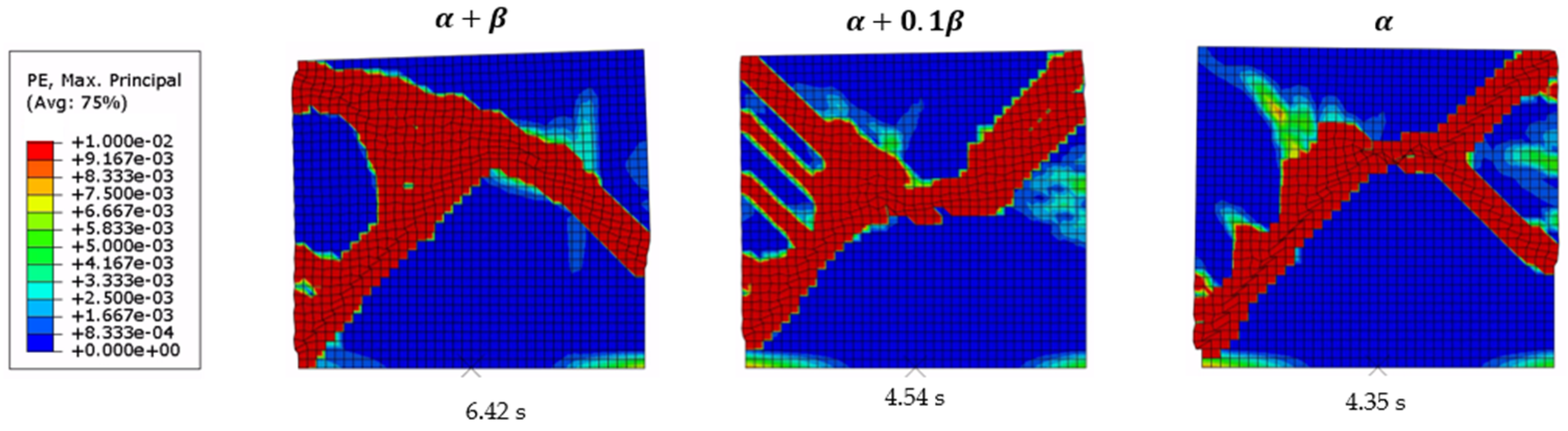
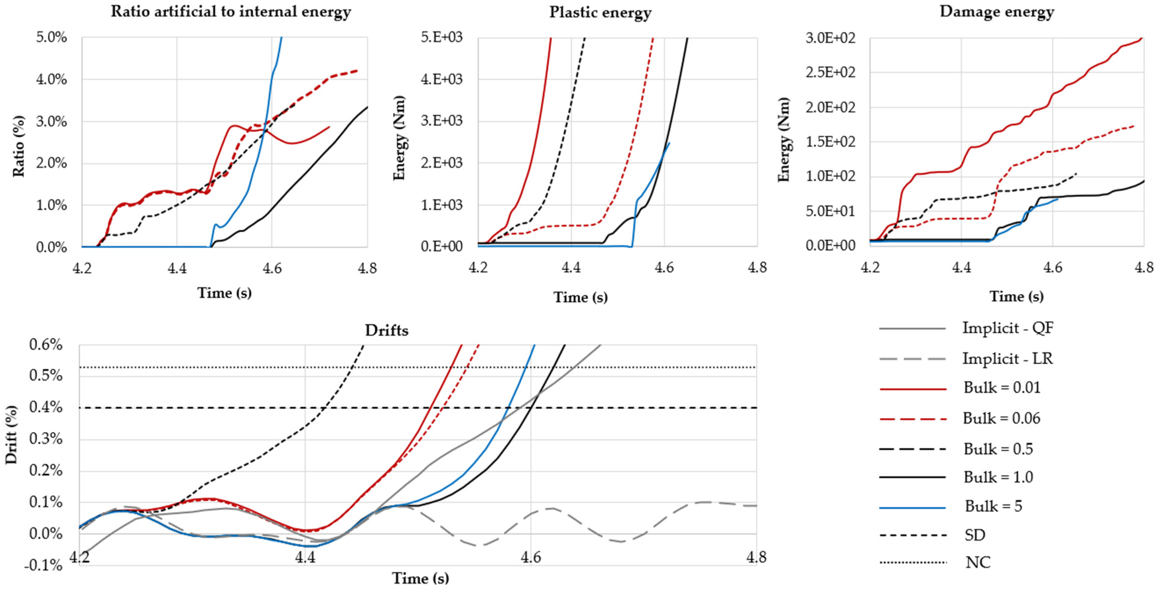
6.3. Parameter 3: Rayleigh Damping in the Explicit Method

Rayleigh damping assumes that the damping matrix C is expressed as a linear combination of the mass M and stiffness K matrices [65], with the form
C = α M + β K
here, α and β are the mass-damping and the stiffness-damping parameters, respectively. For each angular frequency ω a , the damping ratio ξ is related to the Rayleigh damping as
ξ = α 2 ω a + β ω a 2
When considering damping in explicit solvers, the time increment Δ t is determined as follows [94]:
Δ t 2 ω m a x ( 1 + ξ 2 ξ )
where ω m a x is the highest frequency of the system. If ω m a x is high, the term associated with α has a negligible effect on the time increment. Conversely, β can significantly reduce the time step, and it may even make the analysis unfeasible for large models. To address this issue and minimize the computational cost, it is usually to set β to zero and only α is applied [94,95]. This decision is based on the assumption that the structural response is mainly dominated by low frequencies, which are associated with the mass [67]. On the other hand, if β is applied, it is recommended that its value is either of the same order of magnitude or less than the time increment without damping [87]. It is noticed that Abaqus automatically calculates the time increment. The damping ratio was assumed to be 3% for all the models. For the analysis of the piers, three damping conditions for β were tested: equal to zero, with the value calculated according to Equation (10), and a reduction of that value to 10%.

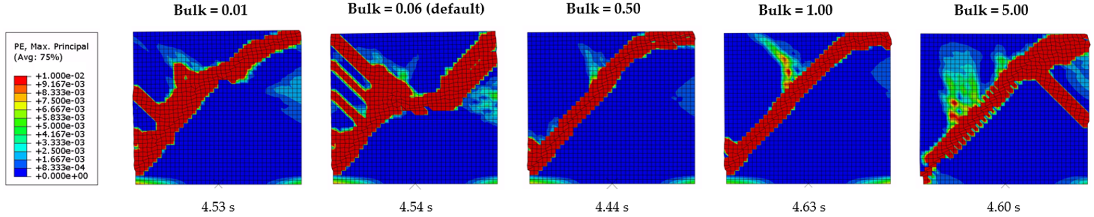
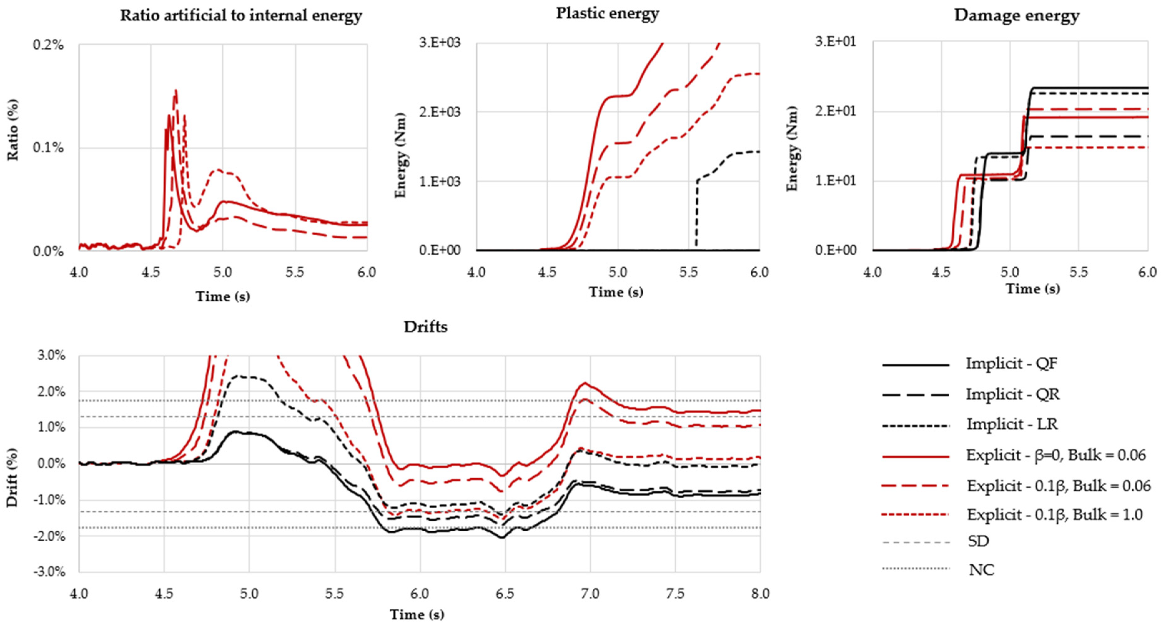
6.4. Parameter 4: Bulk Viscosity in the Explicit Method

In Abaqus, bulk viscosity is used as another method to damp out the structural response [87]. This type of damping is associated with volumetric strain and is intended to control numerical oscillations occurring at the highest frequencies. Bulk viscosity p is defined as a linear function of the volumetric strain rate ε ˙ v o l , and is expressed as:
p = b ρ c d L e ε ˙ v o l
where b is a damping coefficient, ρ  represents the current material density, c d is the current dilatation wave speed, and L e denotes the element’s characteristic length. Six values for b were investigated: 0.01, 0.06 (default value), 0.50, 1.00, 5.00, and 10.00.

7. Seismic Analysis

7.1. Seismic Action

All the models followed the same loading protocol. In order to simulate a quasi-static analysis, the gravitational load was applied with a low velocity using a smooth function. Then, the dynamic analysis was performed by applying the seismic action at the base of the models. In the case of the explicit method, it is more efficient when the dynamic loads are introduced as velocities [87]. The Emilia Romagna earthquake, which is considered to be impulsive, was selected for this work [96]. Figure 11 shows the North–South component in terms of velocities recorded in the seismic station in Mirandola (Italy) on 29 May 2012. The load was incrementally applied until the models exhibited damage.

7.2. Results of the Piers Models

In the initial phase, the implicit method was used to solve the nonlinear dynamic problem, in Abaqus/Standard. Abaqus’ implicit solver offers four element types for plane stress simulations, i.e., linear elements with full (LF) and reduced integration (LR), and quadratic elements with full (QF) and reduced integration (QR). Therefore, the performance of these four element types was evaluated in this stage. Specifically, for the linear elements with reduced integration, three different hourglass control techniques were selected: relax stiffness, (pure) stiffness, and combined. For all three controls, the scaling factor was uniformly set at 0.01.
In the second phase, the explicit solver (Abaqus/Explicit) was used to reproduce the results obtained from the implicit solver. As Abaqus exclusively offers linear elements with reduced integration for plane stress scenarios, this particular element type was uniformly employed throughout all mesh configurations. During this stage, an evaluation of the three hourglass controls was conducted. Subsequently, a third set of analyses allowed an evaluation of the influence of the Rayleigh damping coefficient β on both response and time increment. Finally, the bulk viscosity was tested to evaluate its performance, including its impact on the time increment. The analyses were considered valid if the near-collapse (NC) limit state was attained within the 5% tolerance for artificial energy. A damping ratio of 3% was adopted for all the models.

7.2.1. Pier 1: Shear-Diagonal Failure

Based on preliminary analyses, an amplitude of 75% was determined as a suitable dynamic input for conducting the analyses. In accordance with Eurocode 8 guidelines, two critical limit states based on structural drift are recommended: significant damage (SD) and near collapse (NC). For primary structural elements, the SD limit corresponds to a drift of 0.40%, while the NC limit is set at 0.53% [97]. The drifts were calculated at the midpoint of the top of the pier.
In the first set of analyses, the four element types were tested through the implicit solver. For linear elements with reduced integration, the three hourglass controls were implemented. The fundamental frequency of the model was 7.58 Hz. The time increment was set to 0.005 s and the calculated Rayleigh damping parameters were α = 2.26981 and β = 2.596 × 10⁻⁴. All the models exhibited similar drift responses before the onset of large plastic deformations at approximately 4.5 s (see drifts in Figure 12). Notably, linear elements seemed to be stiffer, particularly the LF model (full integration), which never reached the limit states. The mass on top of the wall also imposed some degree of flexural behaviour on the pier. Therefore, the LF model underestimated the displacements, since linear elements with full integration are stiffer against this deformation type. The employment of a greater number of elements did not alleviate the shear locking effect. Regarding the three models with reduced integration (LR), their behaviour was identical irrespective of the hourglass control applied.
In the CDP constitutive law, the concept of damage energy represents the dissipated energy due to the reduction of material strength, whereas plastic energy refers to the energy required to induce plastic deformations. As seen in Figure 12, when the NC limit was attained, LR models dissipated more energy through plasticity but less through damage compared to QF and QR models. The damage patterns at the NC state, expressed in terms of maximum strains, are depicted in Figure 13. The damage in all the models started at the corners of the base, indicating an initial flexion. However, the predominant failure mode was the abrupt initiation of a diagonal crack, as expected.
The next series of analyses were carried out using the explicit solver. Nine models were created to assess the three selected hourglass controls: relax stiffness, (pure) stiffness, and combined, each with three different scaling factor values: 0.01, 0.02, and 0.03. It is noted that only the α damping parameter was used. The initial time increment automatically calculated by Abaqus was 3.697682 × 10⁻⁵ s.
Figure 14 presents the time history results for these nine models, and for comparison, the responses of the LR and QF models are also included. In this work, it is assumed that the results from quadratic elements with full integration are the more accurate and thus the reference. Models with a scaling factor of 0.03 generated more artificial energy, while the models with 0.01 were more efficient. In nearly all the cases, the NC limit was reached before the artificial energy achieved 5%.
Independently of the hourglass control, the response of the nine models is conservative compared to the implicit solution. Before the material nonlinearities increased considerably at 4.2 s, the drifts were similar to the implicit solution, in particular to the LR model (see drifts in Figure 14). Models with combined hourglass control dissipated more energy through plasticity and damage.
Figure 15 illustrates the damage patterns at the NC state, expressed in terms of maximum strains. The type of hourglass control and the scaling factor value influence the distribution of damage. Nonetheless, the primary failure mode remains consistent: the initiation of a diagonal crack, which aligns with the outcomes from the implicit analyses. For the subsequent analyses, the relax stiffness control with a scaling factor of 0.01 was selected. It is noted that either stiffness or combined controls with the same scaling factor value could have been selected since, overall, their behaviour was similar.
The subsequent phase involves three models to evaluate the influence of the damping parameter β on the solution and time increment. These models were created using the previously selected hourglass control. Three values for β were assigned as follows. Using the Rayleigh formulation, a first value for β was calculated as β = 2.596 × 10⁻⁴. The model is denoted α + β . The second value was set to β = 2.596 × 10⁻⁵, which is a reduction of 10% (denoted α + 0.1 β ). This value also aligns with the same order of magnitude of the initial time increment without damping ( Δ t = 3.70 × 10⁻⁵) [87]. Lastly, β = 0 was applied, in line with common practice. This model is referred as α .
The time history results of the three models are shown in Figure 16. For comparison, the results from the QF and LR are also included. The introduction of the damping parameter β delayed and controlled the increase in artificial energy. Nevertheless, when β is not reduced, the response in terms of displacements is significantly diminished and the initiation of damage is delayed. The models with β = 0 and 0.1 β exhibited comparable levels of energy dissipation (plastic and damage energies) at the NC state.
The primary failure mode in the model with 0.1 β and β = 0 remains consistent with the previous analyses, consisting of the occurrence of a diagonal shear crack, as seen in Figure 17. It is noted that the image corresponding to the model α + β belongs to the last step just before numerical problems arose. Based on these outcomes, the subsequent set of analyses was conducted using the value of 0.1 β .
The time increment for β = 2.596 × 10⁻⁴ was considerably small (see Figure 18). Indeed, using this value not only increases computational time but also yields an unrealistic response (Figure 16). Regarding the model with 0.1 β , there was a minor reduction in the time increment, from Δ t = 3.70 × 10⁻⁵ to Δ t = 2.01 × 10⁻⁵, while the response became closer to the QF model of the implicit method.
In the last series for diagonal shear failure, the effect of the bulk viscosity parameter was assessed, assigning five values: 0.01, 0.06 (by default in Abaqus), 0.50, 1.00, and 5.00. The models were generated using the previously selected relax stiffness equal to 0.01 and β = 2.596 × 10⁻⁵. Since bulk viscosity is a type of damping, it has an impact on the time increment. The reduction became more evident as the value increased, as seen in Figure 18.
In terms of displacements, models with bulk equal to 1.00 and 5.00 behaved similarly to the LR model of the implicit solution. Nevertheless, the onset of the diagonal crack and the subsequent behaviour align more closely with the QF model, as they both approach the NC state nearly simultaneously. Despite the similar responses of both models, the one with a bulk value of 1.00 demonstrated greater stability in terms of artificial energy and computational time. This model reached the NC state before the artificial energy achieved 1.00% (see Figure 19).
Figure 20 depicts the damage patterns at the NC state, where the main failure mode is the abrupt onset of a diagonal shear crack as the one observed in the implicit solution. The model featuring relax stiffness (scaling factor = 0.01), a damping parameter of 0.1 β , and a bulk viscosity equal to 1.00, appears to align more closely with the implicit solution.

7.2.2. Pier 2: Flexural Failure

In this work, the drift values recommended by Eurocode 8 were considered, in which the damage limit states for flexural failure are determined based on the slenderness of the wall. For primary structural elements, the drift is defined as 0.8 ( H 0 / D ) for the SD state, and as 1.06 ( H 0 / D ) for the NC state, where H 0 is the height of the wall and D denotes its horizontal dimension. The values for the analysed pier are 1.32% and 1.75% for SD and NC states, respectively.
To streamline the analysis and reduce the number of studied parameters, the created models only included the features with the best performance in the previous analyses in both implicit and explicit solvers. In the implicit method, linear elements with full integrations (LF) were excluded due to their inaccuracy in simulating bending problems. Thus, both quadratic elements (QF and QR) and linear elements with reduced integration (LR) were employed. The three hourglass controls (relax stiffness, stiffness, and combined) were applied using a scaling factor of 0.01. The fundamental frequency of the wall was 14.16 Hz. The time increment was set to 0.005 s, and the calculated Rayleigh damping parameters were α = 4.79667 and β = 6.826 × 10⁻⁵.
For the explicit solver, the hourglass modes of the three created models were controlled by the relax stiffness method with a scaling factor of 0.01. The first model featured a damping factor of β = 0 and a bulk value of 0.06, as commonly used in practice. The second model included the damping of 0.1 β and a bulk viscosity value of 0.06. For the third model, the damping was set at 0.1 β with a bulk viscosity value of 1.00, which was the combination with better performance in the shear failure analyses.
Figure 21 shows the time history response of all the models. A key observation is that LR models (implicit solver) exhibited identical behaviour in terms of artificial energy, displacements, and damage distribution, irrespective of the applied hourglass control. These models exceeded the NC limit earlier in the analysis. Although the displacements of QF and QR models were similar during almost all seismic loading, the QR model never reached the NC state. Regarding the explicit solution, the artificial energy generated by the three models was negligible. Nevertheless, the hysteretic energy (plastic and damage) at the NC state was considerably larger compared to the implicit models. In terms of displacements, the model with 0.1 β and a bulk viscosity value of 1.00 behaved more similarly to the LR models in the implicit solution.
The damage pattern of all the models is depicted in Figure 22. A uniform and unique crack propagated throughout the base of the wall. Due to the low pre-compression level and the aspect ratio of Pier 2, the failure modes correspond to an IP rocking failure without crushing in the corners. As is evident from both the time history and damage distribution, the models with reduced integration elements reached the NC state in the opposite direction of the models with quadratic elements.
Finally, six additional models were created by varying the hourglass control (stiffness and combined with a scaling factor of 0.01) and using the same variations for β and bulk viscosity. The results showed insignificant differences in terms of artificial energy, with the same response for displacements. Therefore, it can be concluded that, for this case, any of the three hourglass controls can be used to obtain consistent outputs.

7.3. Results of the Viceregal Building Models

The FEM models of the Viceregal building were generated using linear elements with reduced integration, as Abaqus offers this element type specifically for 2D models within the explicit method. The initial choice for hourglass control was the relax stiffness technique, with a value set at 0.01. Additionally, the value of β was reduced to 10%, and bulk viscosity was assumed to be 1.00. These parameters were selected based on the outcomes of the previous analyses. To validate the results, artificial energy was used as a criterion, and a maximum tolerance of 10% was set for this more complex model.
The seismic input was applied in an incremental procedure in all the models until it caused severe damage or numerical problems related to the artificial energy, thereby ensuring the analysis covered a range of loading conditions and dynamic responses.
The damage states of OOP collapses were determined by the method proposed by Doherty et al. [98] for parapets and simply supported walls as deformable bodies, which relies on experimental tests. This approach accounts for the conservation state of the mortar joints at the pivot points. For moderate degradation, the displacements in a trilinear curve are defined by Δ 1 = 0.13 Δ u , Δ 2 = 0.40 Δ u , and Δ u = 2 / 3 t , where t is the thickness of the wall. The displacements Δ 2 and Δ u can be then related to the significant damage (SD) and near-collapse (NC) limit states, respectively. For this particular case, the values are Δ 2 = 0.24 m and Δ u = 0.60 m. Several control points were used for the assessment; however, for sake the of brevity only the displacements at the top of the façade are presented here.

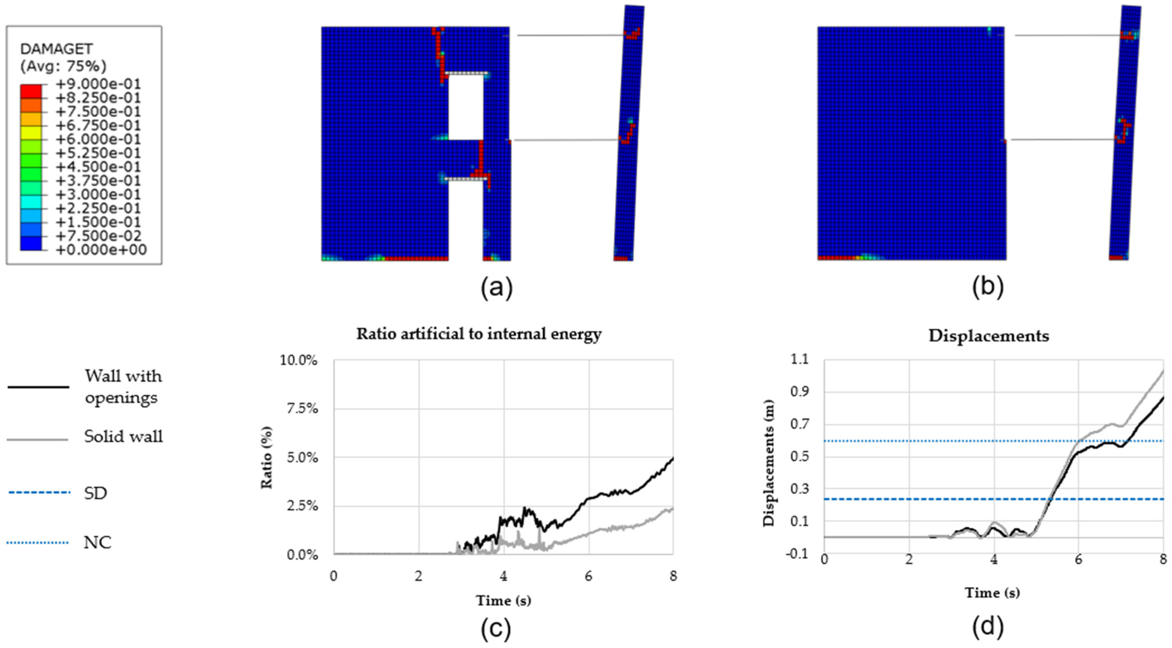
7.3.1. Unreinforced Model

In the preliminary analyses of the Viceregal FEM models, it was observed that the use of relax stiffness had a poor performance in terms of artificial energy. Therefore, relax stiffness control was replaced with stiffness (set at 0.01), as both techniques exhibited similar responses during the shear-diagonal analysis. The stiffness control demonstrated better performance for this more complex dynamic problem. The first mode of vibration corresponded to the OOP motion of the façade. The fundamental frequencies were 1.22 Hz and 1.40 Hz for the model WWO (transversal wall with openings) and for the model SW (solid wall), respectively.
The seismic action was applied with amplitudes ranging from 25 to 75%. At amplitudes below 65%, both models behaved within the elastic range, showing minimal damage, particularly at the base of the façade. Nevertheless, when the amplitude was increased to 75%, the main damage observed was the OOP collapse of the façade (at 6–7 s). The red zones in Figure 23a,b highlight the areas where damage occurred due to tensile stresses at 6.00 s, which, in the CDP model, are defined as the regions where the material experienced a reduction in tensile strength, in this case by 90%. As shown in Figure 23c, the artificial energy remained below 10%, even after the collapse of the façade occurred in both models. Thus, the results can be considered valid. The façades exhibited only outwards OOP displacements, which aligns with the expected behaviour during a real earthquake and highlights the influence of the beams on the direction of the collapse.

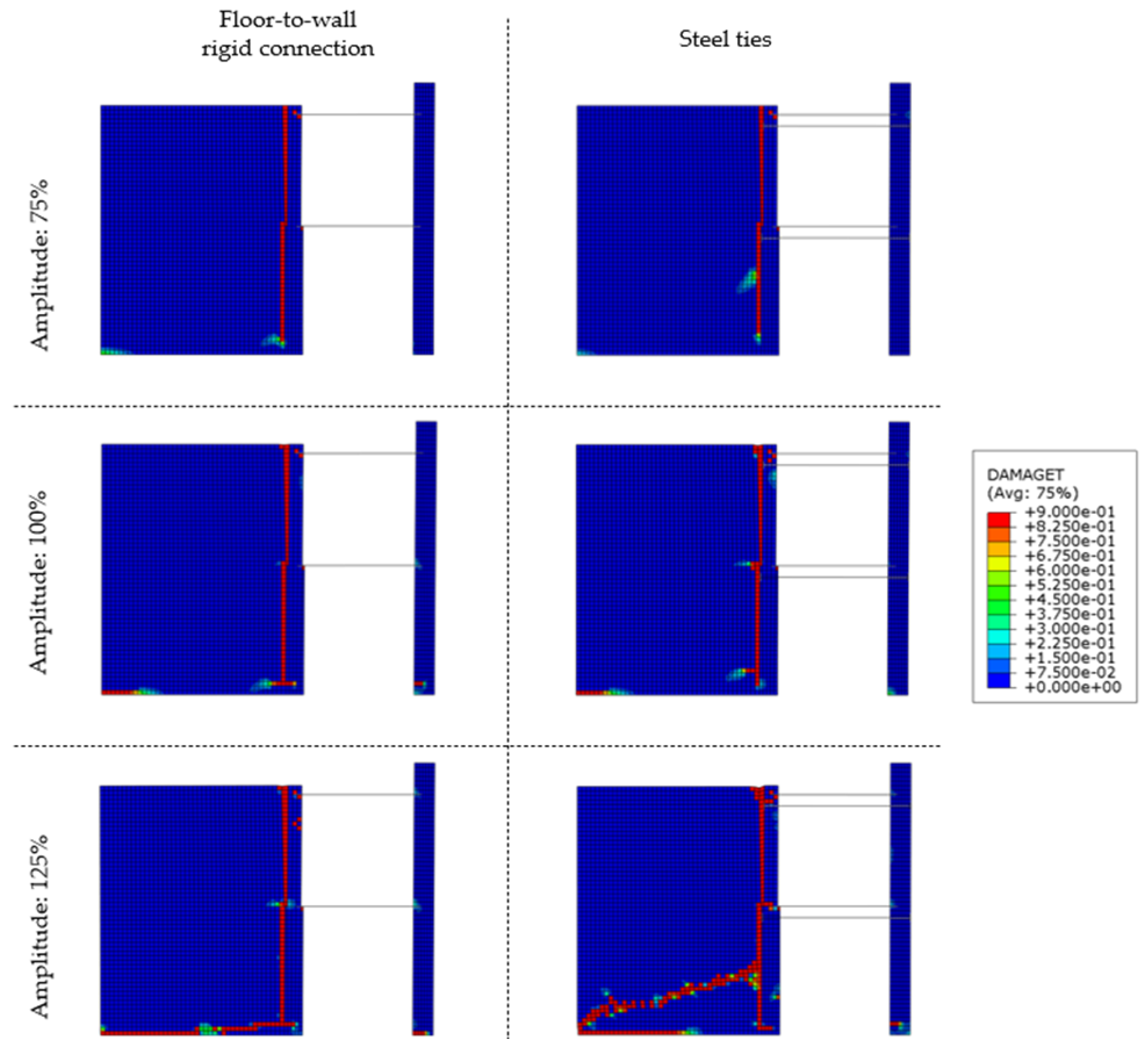
7.3.2. Reinforced Model

Steel tie rods and rigid connections between beams and walls were used to strengthen the structure, since both techniques are considered less invasive and enhance the global seismic performance. The steel components are assumed to behave elastically, with a Young’s modulus of 210 GPa. To limit stress concentrations, steel plates measuring 0.30 × 0.30 m were added at each end of the tie rods. For the reinforced models, the initial amplitude was 75% and gradually increased until considerable damage was caused. As in the previous case, a 10% tolerance in the artificial energy was accepted for the validation of the results.
First, the results of the model representing the façade and the transversal wall with openings (WWO) are discussed. The increment of the fundamental frequencies demonstrated that rigid connections (4.66 Hz) and tie rods (3.44 Hz) increased the stiffness of the model. These frequencies corresponded to the OOP motion of the façade. Figure 24 presents the results at a 75% amplitude for the model WWO. The model strengthened with rigid connections exhibited a numerical problem concerning the artificial energy, and thus the results are assumed to be valid up to 7.50 s. Conversely, the model with ties performed consistently throughout the analysis, below the 10% limit. Tie rods seemed to have a better performance in terms of energy and residual displacements (approximately 0.15 m). This technique induced less damage to the spandrel of the lower level. Although both techniques prevent the OOP collapse of the façade, the inertia forces were transmitted to the transversal wall, resulting in greater base shear forces (see Figure 25).
Further analyses were conducted on the WWO model by increasing the amplitude. At 100%, both models were validated based on the artificial energy criterion. In Figure 25, the tensile damage contours at 6.00 s are presented for amplitudes of 75%, 100%, and 112.5%. The time history results in Figure 26 show that the damage induced by the ties was larger than that caused by the rigid connection of the floor and roof. However, the ties exhibited better control over the OOP displacement of the façade. Additionally, by the end of the analysis, the rigid connection led to more local damage in the façade, resulting in an increase in the damage energy similar to that observed in the case of the tie rods.
In the case of the 112.5% amplitude, the model strengthened with ties maintained stability throughout the entire analysis. In the model with rigid connections, the OOP collapse of the façade occurred before surpassing the energy tolerance at 17.50 s. Hence, the results of both models can be considered reliable. In the model with rigid connections, vertical cracks developed in the spandrels, leading to the complete detachment of the transversal wall from the façade, culminating in its subsequent collapse. The extent of the damaged zone was larger when using rigid connections compared to ties.
For the 112.5% amplitude scenario with ties, the shear-diagonal damage did not appear. This was due to the façade’s damage occurring before the full transmission of the inertia forces to the transversal wall could take place. At the end of the analysis, both spandrels collapsed and the façade exceeded the significant damage limit state with a residual displacement of 0.37 m. Finally, it is worth mentioning that both strengthening techniques induce large shear forces in the transversal wall.
Next, the seismic performance of the model featuring a solid transversal wall (SW) is explained. The first mode of the model corresponded to the OOP motion of the façade with a frequency of 5.55 Hz for the model with rigid connections and 3.62 Hz for the model with tie rods. Figure 27 depicts the comparison between the unreinforced with the reinforced models subjected to an earthquake with 75% amplitude. The low levels of artificial energy ensured the reliability of the results. Although the rigid connections led to damage over a larger area, both techniques exhibited good performance by substantially limiting the OOP motion of the façade, resulting in a residual deformation of less than 0.10 m at the end of the analysis. In the two strengthening scenarios, the tensile strength was reduced by 90% in the transition area between the transversal wall and the wall parallel to the façade (see Figure 28).
The seismic action was gradually increased until achieving an amplitude of 125%. The results are accepted as reliable based on the artificial energy criterion. In all the seismic scenarios and regardless of the adopted strengthening technique, the façade exhibited minimal damage. However, this fact implies that the inertia forces were transferred to other structural components, leading to a degradation of the tensile strength (by 90%) in the intersection of the transversal wall with that parallel to the façade (depicted in Figure 28). The damage caused by the ties is relatively less (for 100% amplitude) or similar (for 125% amplitude) compared to rigid connections, while still providing more effective control on the OOP motion of the façade, as shown in the plots (Figure 29). By the end of the analyses, cracks developed around the beams in the cases where rigid connections were used. For the applied amplitude of 125%, irrespective of the technique, the inertia forces transmitted from the façade triggered severe shear cracks along the entire length of the transversal wall, close to the base (Figure 28).

8. Conclusions

Implicit solvers may encounter convergence issues, especially with materials exhibiting softening behaviour. Furthermore, nonlinear dynamic analysis can be computationally demanding. Explicit solvers offer a solution to these challenges, but their application in seismic analysis, especially for URM structures, is limited. Therefore, the sensitivity analysis herein presented intends to aid users in the framework of explicit solutions. It offers insights into the parameters applicable to dynamic analysis and their impact on the results.
In this work, several models were created using only plane stress elements. Subsequently, a large set of numerical analyses was conducted within the explicit solver of Abaqus. The solutions were then compared with outputs generated by the implicit solver. The findings showed that the nonlinear dynamic response is significantly affected by the element type (quadratic or linear with full or reduced integration) rather than by the specific time integration solver (explicit or implicit method) applied to solve the equations, mainly when strong nonlinearities start to rise.
In the explicit method, the models with damping parameter β = 0 are conservative. A response more aligned with the implicit solution can be achieved by setting the damping to 0.1 β , and by increasing the bulk viscosity value to 1.00. In this regard, the bulk viscosity has less impact on the time increment than the β damping parameter. When using elements with reduced integration for dynamic analyses, assessing the increment of artificial energy plays a key role. The tolerance range of 5–10% appears to be acceptable. For models in the explicit solver, the three hourglass controls performed better in terms of artificial energy when their scaling factor was set to 0.01. No notable difference was observed for simple models. However, for models with more complexity, stiffness hourglass control seemed to be more efficient than relax stiffness and combined controls. It is worth noting that these conclusions are only applicable to plane stress elements. Future works should consider a reliability analysis that includes other variables, such as seismic actions with diverse characteristics, OOP response, and 3D models built with solid elements. Furthermore, a validation of the parameters through the simulation of experimental campaigns, especially shake table tests, should be considered.
With the onset of high nonlinearities (crack formation, material softening, and large displacements) all the numerical techniques started to diverge. However, a majority of these techniques were able to simulate the damage patterns at the NC state. Explicit methods are a promising tool for studying complex buildings that require extensive nonlinear dynamic analyses. In this regard, the reduction in computational time becomes more noticeable as the size of the model increases.

Author Contributions

Conceptualization, E.N.-M. and N.M.; Data curation, E.N.-M. and N.M.; Formal analysis, E.N.-M.; Funding acquisition, N.M.; Methodology, E.N.-M. and N.M.; Project administration, N.M.; Software, V.C. and S.O.; Supervision, N.M.; Validation, E.N.-M. and N.M.; Visualization, E.N.-M., V.C. and S.O.; Writing—original draft, E.N.-M., V.C. and S.O.; Writing—review & editing, N.M. All authors have read and agreed to the published version of the manuscript.

Funding

This work was funded by FCT—Foundation for Science and Technology within the scope of project EXPL/ECI-EGC/0940/2021. The first author is grateful for the funding from the Mexican National Council for Science and Technology (Consejo Nacional de Ciencia y Tecnología CONACYT), grant number 2018-000013-01EXTF-00137.

Institutional Review Board Statement

Not applicable.

Informed Consent Statement

Not applicable.

Data Availability Statement

The data presented in this study are available on request from the corresponding author.

Conflicts of Interest

The authors declare that they have no known competing financial interest or personal relationships that could have appeared to influence the work reported in this paper.

References

  1. Vlachakis, G.; Vlachaki, E.; Lourenço, P.B. Learning from Failure: Damage and Failure of Masonry Structures, after the 2017 Lesvos Earthquake (Greece). Eng. Fail. Anal. 2020, 117, 104803. [Google Scholar] [CrossRef]
  2. Liu, Z.; Crewe, A. Effects of Size and Position of Openings on In-Plane Capacity of Unreinforced Masonry Walls. Bull. Earthq. Eng. 2020, 18, 4783–4812. [Google Scholar] [CrossRef]
  3. Gkournelos, P.D.; Triantafillou, T.C.; Bournas, D.A. Seismic Upgrading of Existing Masonry Structures: A State-of-the-Art Review. Soil Dyn. Earthq. Eng. 2022, 161, 107428. [Google Scholar] [CrossRef]
  4. De Felice, G.; De Santis, S.; Lourenço, P.B.; Mendes, N. Methods and Challenges for the Seismic Assessment of Historic Masonry Structures. Int. J. Archit. Herit. 2016, 11, 143–160. [Google Scholar] [CrossRef]
  5. Ferreira, T.M.; Costa, A.A.; Vicente, R.; Varum, H. A Simplified Four-Branch Model for the Analytical Study of the out-of-Plane Performance of Regular Stone URM Walls. Eng. Struct. 2015, 83, 140–153. [Google Scholar] [CrossRef]
  6. Griffith, M.C.; Magenes, G.; Melis, G.; Picchi, L. Evaluation of Out-of-Plane Stability of Unreinforced Masonry Walls Subjected to Seismic Excitation. J. Earthq. Eng. 2003, 7, 141–169. [Google Scholar] [CrossRef]
  7. Tomazevic, M. Earthquake-Resistant Design of Masonry Buildings; Series on Innovation in Structures and Construction; Imperial College Press and World Scientific Publishing Co.: London, UK, 1999; Volume 1, ISBN 978-1-86094-066-8. [Google Scholar]
  8. Mendes, N.; Lourenço, P.B. Chapter 4—Seismic Assessment of Historic Masonry Structures: Out-of-Plane Effects. In Numerical Modeling of Masonry and Historical Structures; Ghiassi, B., Milani, G., Eds.; Woodhead Publishing: Sawston, UK, 2019; pp. 141–162. ISBN 978-0-08-102439-3. [Google Scholar]
  9. Szabó, S.; Funari, M.F.; Lourenço, P.B. Masonry Patterns’ Influence on the Damage Assessment of URM Walls: Current and Future Trends. Dev. Built Environ. 2023, 13, 100119. [Google Scholar] [CrossRef]
  10. Ortega, J.; Vasconcelos, G.; Rodrigues, H.; Correia, M.; Lourenço, P.B. Traditional Earthquake Resistant Techniques for Vernacular Architecture and Local Seismic Cultures: A Literature Review. J. Cult. Herit. 2017, 27, 181–196. [Google Scholar] [CrossRef]
  11. D’Altri, A.M.; Sarhosis, V.; Milani, G.; Rots, J.; Cattari, S.; Lagomarsino, S.; Sacco, E.; Tralli, A.; Castellazzi, G.; De Miranda, S. Modeling Strategies for the Computational Analysis of Unreinforced Masonry Structures: Review and Classification. Arch. Comput. Methods Eng. 2020, 27, 1153–1185. [Google Scholar] [CrossRef]
  12. Lourenço, P.B. Recent Advances in Masonry Modelling: Micromodelling and Homogenisation. In Multiscale Modeling in Solid Mechanics; Computational and Experimental Methods in Structures; Imperial College Press: London, UK, 2009; Volume 3, pp. 251–294. ISBN 978-1-84816-307-2. [Google Scholar]
  13. Ghiassi, B.; Vermelfoort, A.T.; Lourenço, P.B. Chapter 7—Masonry Mechanical Properties. In Numerical Modeling of Masonry and Historical Structures; Ghiassi, B., Milani, G., Eds.; Woodhead Publishing: Sawston, UK, 2019; pp. 239–261. ISBN 978-0-08-102439-3. [Google Scholar]
  14. Pereira, J.M.; Campos, J.; Lourenço, P.B. Masonry Infill Walls under Blast Loading Using Confined Underwater Blast Wave Generators (WBWG). Eng. Struct. 2015, 92, 69–83. [Google Scholar] [CrossRef]
  15. Pereira, J.M.; Lourenço, P.B. Risk Assessment Due to Terrorist Actions on Public Transportation Networks: A Case Study in Portugal. Int. J. Prot. Struct. 2014, 5, 391–415. [Google Scholar] [CrossRef]
  16. Tse, D.; Pereira, J.M.; Lourenço, P.B. Numerical Analysis of an Earthen Masonry Structure Subjected to Blast Loading. CivilEng 2021, 2, 969–985. [Google Scholar] [CrossRef]
  17. Tarque, N.; Camata, G.; Spacone, E.; Varum, H.; Blondet, M. Nonlinear Dynamic Analysis of a Full-Scale Unreinforced Adobe Model. Earthq. Spectra 2014, 30, 1643–1661. [Google Scholar] [CrossRef]
  18. Yang, B. Comparisons of Implicit and Explicit Time Integration Methods in Finite Element Analysis for Linear Elastic Material and Quasi-Brittle Material in Dynamic Problems. Master’s Thesis, Delft University of Technology, Delf, The Netherlands, 2019. [Google Scholar]
  19. Noor-E-Khuda, S.; Dhanasekar, M.; Thambiratnam, D.P. An Explicit Finite Element Modelling Method for Masonry Walls under Out-of-Plane Loading. Eng. Struct. 2016, 113, 103–120. [Google Scholar] [CrossRef]
  20. Lourenço, P.B.; Gaetani, A. Finite Element Analysis for Building Assessment: Advanced Use and Practical Recommendations, 1st ed.; Routledge: New York, NY, USA, 2022; ISBN 978-0-429-34156-4. [Google Scholar]
  21. Weber, M.; Thoma, K.; Hofmann, J. Finite Element Analysis of Masonry under a Plane Stress State. Eng. Struct. 2021, 226, 111214. [Google Scholar] [CrossRef]
  22. D’Altri, A.M.; Cannizzaro, F.; Petracca, M.; Talledo, D.A. Nonlinear Modelling of the Seismic Response of Masonry Structures: Calibration Strategies. Bull. Earthq. Eng. 2022, 20, 1999–2043. [Google Scholar] [CrossRef]
  23. Dassault Systèmes. Abaqus/CAE 2019; Dassault Systèmes Simulia Corp.: Johnston, RI, USA, 2018. [Google Scholar]
  24. Frumento, S.; Giovinazzi, S.; Lagomarsino, S.; Podestà, S. Seismic Retrofitting of Unreinforced Masonry Buildings in Italy; Springer: Napier, New Zeland, 2006. [Google Scholar]
  25. Oliveira, D.V.; Silva, R.A.; Garbin, E.; Lourenço, P.B. Strengthening of Three-Leaf Stone Masonry Walls: An Experimental Research. Mater. Struct. 2012, 45, 1259–1276. [Google Scholar] [CrossRef]
  26. Candeias, P. Avaliação da Vulnerabilidade Sísmica de Edifícios de Alvenaria. Ph.D. Thesis, University of Minho, Lisboa, Portugal, 2010. [Google Scholar]
  27. Vintzileou, E. Three-Leaf Masonry in Compression, Before and After Grouting: A Review of Literature. Int. J. Archit. Herit. 2011, 5, 513–538. [Google Scholar] [CrossRef]
  28. Corradi, M.; Borri, A.; Poverello, E.; Castori, G. The Use of Transverse Connectors as Reinforcement of Multi-Leaf Walls. Mater. Struct. 2017, 50, 114. [Google Scholar] [CrossRef]
  29. Bhattacharya, S.; Nayak, S.; Dutta, S.C. A Critical Review of Retrofitting Methods for Unreinforced Masonry Structures. Int. J. Disaster Risk Reduct. 2014, 7, 51–67. [Google Scholar] [CrossRef]
  30. Valluzzi, M.R.; Modena, C.; De Felice, G. Current Practice and Open Issues in Strengthening Historical Buildings with Composites. Mater. Struct. 2014, 47, 1971–1985. [Google Scholar] [CrossRef]
  31. Abbass, A.; Lourenço, P.B.; Oliveira, D.V. The Use of Natural Fibers in Repairing and Strengthening of Cultural Heritage Buildings. Mater. Today Proc. 2020, 31, S321–S328. [Google Scholar] [CrossRef]
  32. Papanicolaou, C.G.; Triantafillou, T.C.; Karlos, K.; Papathanasiou, M. Textile-Reinforced Mortar (TRM) versus FRP as Strengthening Material of URM Walls: In-Plane Cyclic Loading. Mater. Struct. 2007, 40, 1081–1097. [Google Scholar] [CrossRef]
  33. Babaeidarabad, S.; Caso, F.D.; Nanni, A. Out-of-Plane Behavior of URM Walls Strengthened with Fabric-Reinforced Cementitious Matrix Composite. J. Compos. Constr. 2014, 18, 04013057. [Google Scholar] [CrossRef]
  34. Papanicolaou, C.G.; Triantafillou, T.C.; Papathanasiou, M.; Karlos, K. Textile Reinforced Mortar (TRM) versus FRP as Strengthening Material of URM Walls: Out-of-Plane Cyclic Loading. Mater. Struct. 2007, 41, 143–157. [Google Scholar] [CrossRef]
  35. Federal Emergency Management Agency (FEMA). Techniques for the Seismic Rehabilitation of Existing Buildings; Federal Emergency Management Agency (FEMA): Washington, DC, USA, 2006. [Google Scholar]
  36. Ferreira, T.M.; Mendes, N.; Silva, R. Multiscale Seismic Vulnerability Assessment and Retrofit of Existing Masonry Buildings. Buildings 2019, 9, 91. [Google Scholar] [CrossRef]
  37. Borri, A.; Castori, G.; Grazini, A. Retrofitting of Masonry Building with Reinforced Masonry Ring-Beam. Constr. Build. Mater. 2009, 23, 1892–1901. [Google Scholar] [CrossRef]
  38. Valluzzi, M.R.; Garbin, E.; Benetta, M.D. In-Plane Strengthening of Timber Floors for the Seismic Improvement of Masonry Buildings; Springer: Berlin/Heidelberg, Germany, 2010. [Google Scholar]
  39. Senaldi, I.; Magenes, G.; Penna, A.; Galasco, A.; Rota, M. The Effect of Stiffened Floor and Roof Diaphragms on the Experimental Seismic Response of a Full-Scale Unreinforced Stone Masonry Building. J. Earthq. Eng. 2014, 18, 407–443. [Google Scholar] [CrossRef]
  40. Solarino, F.; Oliveira, D.V.; Giresini, L. Wall-to-Horizontal Diaphragm Connections in Historical Buildings: A State-of-the-Art Review. Eng. Struct. 2019, 199, 109559. [Google Scholar] [CrossRef]
  41. Angulo-Ibáñez, Q.; Mas-Tomás, Á.; Galvañ-LLopis, V.; Sántolaria-Montesinos, J.L. Traditional Braces of Earth Constructions. Constr. Build. Mater. 2012, 30, 389–399. [Google Scholar] [CrossRef]
  42. Lucibello, G.; Brandonisio, G.; Mele, E.; De Luca, A. Seismic Damage and Performance of Palazzo Centi after L’Aquila Earthquake: A Paradigmatic Case Study of Effectiveness of Mechanical Steel Ties. Eng. Fail. Anal. 2013, 34, 407–430. [Google Scholar] [CrossRef]
  43. Nochebuena-Mora, E.; Mendes, N.; Lourenço, P.B.; Covas, J.A. Vibration Control Systems: A Review of Their Application to Historical Unreinforced Masonry Buildings. J. Build. Eng. 2021, 44, 103333. [Google Scholar] [CrossRef]
  44. Saaed, T.E.; Nikolakopoulos, G.; Jonasson, J.-E.; Hedlund, H. A State-of-the-Art Review of Structural Control Systems. J. Vib. Control 2015, 21, 919–937. [Google Scholar] [CrossRef]
  45. Warn, G.P.; Ryan, K.L. A Review of Seismic Isolation for Buildings: Historical Development and Research Needs. Buildings 2012, 2, 300–325. [Google Scholar] [CrossRef]
  46. Symans, M.D.; Charney, F.A.; Whittaker, A.S.; Constantinou, M.C.; Kircher, C.A.; Johnson, M.W.; McNamara, R.J. Energy Dissipation Systems for Seismic Applications: Current Practice and Recent Developments. J. Struct. Eng. 2008, 134, 3–21. [Google Scholar] [CrossRef]
  47. Martínez-Rueda, J.E. On the Evolution of Energy Dissipation Devices for Seismic Design. Earthq. Spectra 2002, 18, 309–346. [Google Scholar] [CrossRef]
  48. Lockrem, R.; Schuller, M.; Locke, R. Modifying Building Response Using Energy Absorbing Diaphragm-to-Wall Connectors. In Proceedings of the 4th International Seminar on Structural Analysis of Historic Constructions 2004; Modena, C., Lourenço, P.B., Roca, P., Eds.; Taylor & Francis Group: Padova, Italy, 2005; pp. 1215–1220. [Google Scholar]
  49. Preti, M.; Loda, S.; Bolis, V.; Cominelli, S.; Marini, A.; Giuriani, E. Dissipative Roof Diaphragm for the Seismic Retrofit of Listed Masonry Churches. J. Earthq. Eng. 2019, 23, 1241–1261. [Google Scholar] [CrossRef]
  50. D’Ayala, D.F.; Paganoni, S. Testing and Design Protocol of Dissipative Devices for Out-of-Plane Damage. Proc. Inst. Civ. Eng.—Struct. Build. 2014, 167, 26–40. [Google Scholar] [CrossRef]
  51. Alam, M.S.; Youssef, M.A.; Nehdi, M. Utilizing Shape Memory Alloys to Enhance the Performance and Safety of Civil Infrastructure: A Review. Can. J. Civ. Eng. 2007, 34, 1075–1086. [Google Scholar] [CrossRef]
  52. Indirli, M.; Castellano, M.G. Shape Memory Alloy Devices for the Structural Improvement of Masonry Heritage Structures. Int. J. Archit. Herit. 2008, 2, 93–119. [Google Scholar] [CrossRef]
  53. Giresini, L.; Solarino, F.; Taddei, F.; Mueller, G. Experimental Estimation of Energy Dissipation in Rocking Masonry Walls Restrained by an Innovative Seismic Dissipator (LICORD). Bull. Earthq. Eng. 2021, 19, 2265–2289. [Google Scholar] [CrossRef]
  54. Addessi, D.; Marfia, S.; Sacco, E. Chapter 10—Homogenization and Multiscale Analysis. In Numerical Modeling of Masonry and Historical Structures; Ghiassi, B., Milani, G., Eds.; Woodhead Publishing: Sawston, UK, 2019; pp. 351–395. ISBN 978-0-08-102439-3. [Google Scholar]
  55. Caddemi, S.; Caliò, I.; Cannizzaro, F.; Pantò, B.; Rapicavoli, D. Chapter 14—Descrete Macroelement Modeling. In Numerical Modeling of Masonry and Historical Structures; Ghiassi, B., Milani, G., Eds.; Woodhead Publishing: Sawston, UK, 2019; pp. 503–533. ISBN 978-0-08-102439-3. [Google Scholar]
  56. Massart, T.J.; Ehab Moustafa Kamel, K.; Hernandez, H. Chapter 11—Automated Geometry Extraction and Discretization for Cohesive Zone-Based Modeling of Irregular Masonry. In Numerical Modeling of Masonry and Historical Structures; Ghiassi, B., Milani, G., Eds.; Woodhead Publishing: Sawston, UK, 2019; pp. 397–422. ISBN 978-0-08-102439-3. [Google Scholar]
  57. Milani, G.; Taliercio, A. Chapter 12—Homogenization Limit Analysis. In Numerical Modeling of Masonry and Historical Structures; Ghiassi, B., Milani, G., Eds.; Woodhead Publishing: Sawston, UK, 2019; pp. 423–467. ISBN 978-0-08-102439-3. [Google Scholar]
  58. Minga, E.; Macorini, L.; Izzuddin, B.A.; Calio’, I. Chapter 8—Macromodeling. In Numerical Modeling of Masonry and Historical Structures; Ghiassi, B., Milani, G., Eds.; Woodhead Publishing: Sawston, UK, 2019; pp. 263–294. ISBN 978-0-08-102439-3. [Google Scholar]
  59. Sarhosis, V.; Lemos, J.V.; Bagi, K. Chapter 13—Discrete Element Modeling. In Numerical Modeling of Masonry and Historical Structures; Ghiassi, B., Milani, G., Eds.; Woodhead Publishing: Sawston, UK, 2019; pp. 469–501. ISBN 978-0-08-102439-3. [Google Scholar]
  60. Rekik, A.; Lebon, F. Chapter 9—Micromodeling. In Numerical Modeling of Masonry and Historical Structures; Ghiassi, B., Milani, G., Eds.; Woodhead Publishing: Sawston, UK, 2019; pp. 295–349. ISBN 978-0-08-102439-3. [Google Scholar]
  61. Smoljanović, H.; Živaljić, N.; Nikolić, Ž. A Combined Finite-Discrete Element Analysis of Dry Stone Masonry Structures. Eng. Struct. 2013, 52, 89–100. [Google Scholar] [CrossRef]
  62. Lemos, J.V. Discrete Element Modeling of Masonry Structures. Int. J. Archit. Herit. 2007, 1, 190–213. [Google Scholar] [CrossRef]
  63. Belmouden, Y.; Lestuzzi, P. An Equivalent Frame Model for Seismic Analysis of Masonry and Reinforced Concrete Buildings. Constr. Build. Mater. 2009, 23, 40–53. [Google Scholar] [CrossRef]
  64. Petrovčič, S.; Kilar, V. Seismic Failure Mode Interaction for the Equivalent Frame Modeling of Unreinforced Masonry Structures. Eng. Struct. 2013, 54, 9–22. [Google Scholar] [CrossRef]
  65. Chopra, A.K. Dynamics of Structures: Theory and Applications to Earthquake Engineering, 4th ed.; Prentice Hall: Upper Saddle River, NJ, USA, 2015; ISBN 978-0-273-77424-2. [Google Scholar]
  66. Clough, R.W.; Penzien, J. Dynamic of Structures, 3rd ed.; Computers & Structures: Berkeley, CA, USA, 2003. [Google Scholar]
  67. Dokainish, M.A.; Subbaraj, K. A Survey of Direct Time-Integration Methods in Computational Structural Dynamics—I. Explicit Methods. Comput. Struct. 1989, 32, 1371–1386. [Google Scholar] [CrossRef]
  68. Hilber, H.M.; Hughes, T.J.R.; Taylor, R.L. Improved Numerical Dissipation for Time Integration Algorithms in Structural Dynamics. Earthq. Eng. Struct. Dyn. 1977, 5, 283–292. [Google Scholar] [CrossRef]
  69. Subbaraj, K.; Dokainish, M.A. A Survey of Direct Time-Integration Methods in Computational Structural Dynamics—II. Implicit Methods. Comput. Struct. 1989, 32, 1387–1401. [Google Scholar] [CrossRef]
  70. Wu, S.R.; Gu, L. Introduction to the Explicit Finite Element Method for Nonlinear Transient Dynamics; John Wiley & Sons, Ltd.: Hoboken, NJ, USA, 2012; ISBN 978-1-118-38201-1. [Google Scholar]
  71. Appleton, J.G. Reabilitação de Edifícios “Gaioleiros”, 1st ed.; Orion: Lisboa, Portugal, 2005; ISBN 972-8620-05-5. [Google Scholar]
  72. Simões, A.G.; Appleton, J.G.; Bento, R.; Caldas, J.V.; Lourenço, P.B.; Lagomarsino, S. Architectural and Structural Characteristics of Masonry Buildings between the 19th and 20th Centuries in Lisbon, Portugal. Int. J. Archit. Herit. 2017, 11, 457–474. [Google Scholar] [CrossRef]
  73. Bühler, D. Puebla, Patrimonio de Arquitectura Civil del Virreinato, 1st ed.; Deutsches Museum ICOMOS: München, Germany, 2001; ISBN 3-924183-81-3. [Google Scholar]
  74. Barrera Barrera, M. Los Inmuebles Habitacionales en Valladolid de Michoacán, Siglo XVIII, Sistemas Constructivos y Proporcionamiento del Espacio.pdf. Master’s Thesis, Universidad Michoacana de San Nicolás de Hidalgo, Morelia, Mexico, 2012. [Google Scholar]
  75. González Avellaneda, A.; Hueytletl Torres, A.; Pérez Méndez, B.; Ramos Molina, L.; Salazar Muñoz, V. Manual Técnico de Procedimientos para la Rehabilitación de Monumentos Históricos en el Distrito Federal, 1st ed.; Instituto Nacional de Antropología e Historia: Ciudad de México, Mexico, 1988. [Google Scholar]
  76. Ministry of Infrastructure and Transport Circolare 2019 Instruction for the Application of the Building Code for Constructions; Aggiornamento delle “Norme tecniche per le costruzioni”: Roma, Italy, 2019.
  77. Dassault Systèmes. Abaqus Theory Guide, Version 6.14.; Dassault Systèmes Simulia Corp.: Providence, RI, USA, 2014. Available online: http://130.149.89.49:2080/v6.14/books/stm/default.htm(accessed on 14 August 2023).
  78. Acito, M.; Bocciarelli, M.; Chesi, C.; Milani, G. Collapse of the Clock Tower in Finale Emilia after the May 2012 Emilia Romagna Earthquake Sequence: Numerical Insight. Eng. Struct. 2014, 72, 70–91. [Google Scholar] [CrossRef]
  79. Tiberti, S.; Acito, M.; Milani, G. Comprehensive FE Numerical Insight into Finale Emilia Castle Behavior under 2012 Emilia Romagna Seismic Sequence: Damage Causes and Seismic Vulnerability Mitigation Hypothesis. Eng. Struct. 2016, 117, 397–421. [Google Scholar] [CrossRef]
  80. Castellazzi, G.; D’Altri, A.M.; De Miranda, S.; Chiozzi, A.; Tralli, A. Numerical Insights on the Seismic Behavior of a Non-Isolated Historical Masonry Tower. Bull. Earthq. Eng. 2018, 16, 933–961. [Google Scholar] [CrossRef]
  81. Valente, M. Seismic Behavior and Damage Assessment of Two Historical Fortified Masonry Palaces with Corner Towers. Eng. Fail. Anal. 2022, 134, 106003. [Google Scholar] [CrossRef]
  82. Valente, M. Earthquake Response and Damage Patterns Assessment of Two Historical Masonry Churches with Bell Tower. Eng. Fail. Anal. 2023, 151, 107418. [Google Scholar] [CrossRef]
  83. Lubliner, J.; Oliver, J.; Oller, S.; Oñate, E. A Plastic-Damage Model for Concrete. Int. J. Solids Struct. 1989, 25, 299–326. [Google Scholar] [CrossRef]
  84. Lee, J.; Fenves, G.L. Plastic-Damage Model for Cyclic Loading of Concrete Structures. J. Eng. Mech. 1998, 124, 892–900. [Google Scholar] [CrossRef]
  85. Chi, Y.; Yu, M.; Huang, L.; Xu, L. Finite Element Modeling of Steel-Polypropylene Hybrid Fiber Reinforced Concrete Using Modified Concrete Damaged Plasticity. Eng. Struct. 2017, 148, 23–35. [Google Scholar] [CrossRef]
  86. Feenstra, P.H. Computational Aspects of Biaxial Stress in Plain and Reinforced Concrete. Ph.D. Thesis, Delft University of Technology, Delft, The Netherlands, 1993. [Google Scholar]
  87. Dassault Systèmes. Abaqus Analysis User’s Guide, Version 6.14.; Dassault Systèmes Simulia Corp.: Providence, RI, USA, 2014. Available online: http://130.149.89.49:2080/v6.14/books/usb/default.htm(accessed on 14 August 2023).
  88. AlGohi, B.H.; Baluch, M.H.; Rahman, M.K.; Al-Gadhib, A.H.; Demir, C. Plastic-Damage Modeling of Unreinforced Masonry Walls (URM) Subject to Lateral Loading. Arab. J. Sci. Eng. 2017, 42, 4201–4220. [Google Scholar] [CrossRef]
  89. Dassault Systèmes. Getting Started with Abaqus: Interactive Edition, Version 6.14.; Dassault Systèmes Simulia Corp.: Providence, RI, USA, 2014. Available online: http://130.149.89.49:2080/v6.14/books/gsa/default.htm(accessed on 14 August 2023).
  90. Martin, O. Comparison of Different Constitutive Models for Concrete in ABAQUS/Explicit for Missile Impact Analyses; European Commission Joint Research Centre Institute for EnergyPublications Office: Luxembourg, 2010; ISBN 978-92-79-14988-7. [Google Scholar]
  91. Boulbes, R.J. Troubleshooting Finite-Element Modeling with Abaqus: With Application in Structural Engineering Analysis; Springer Cham: Cham, Switzerland, 2020; ISBN 978-3-030-26739-1. [Google Scholar]
  92. Storheim, M.; Notaro, G.; Johansen, A.; Amdahl, J. Comparison of ABAQUS and LS-DYNA in Simulations of Ship Collisions. In Proceedings of the ICCGS 2016, Ulsan, Republic of Korea, 15–18 June 2016. [Google Scholar]
  93. Zheng, G.; Nie, H.; Chen, J.; Chen, C.; Lee, H.P. Dynamic Analysis of Lunar Lander during Soft Landing Using Explicit Finite Element Method. Acta Astronaut. 2018, 148, 69–81. [Google Scholar] [CrossRef]
  94. Lemos, J.V.; Dawson, E.M.; Cheng, Z. Application of Maxwell Damping in the Dynamic Analysis of Masonry Structures with Discrete Elements. Int. J. Mason. Res. Innov. 2022, 7, 663–686. [Google Scholar] [CrossRef]
  95. Chen, X.M.; Duan, J.; Qi, H.; Li, Y.G. Rayleigh Damping in Abaqus/Explicit Dynamic Analysis. Appl. Mech. Mater. 2014, 627, 288–294. [Google Scholar] [CrossRef]
  96. Bianchini, N.; Mendes, N.; Calderini, C.; Lourenço, P.B. Modelling of the Dynamic Response of a Reduced Scale Dry Joints Groin Vault. J. Build. Eng. 2023, 66, 105826. [Google Scholar] [CrossRef]
  97. CEN EN 1998-3 (2005); Eurocode 8: Design of Structures for Earthquake Resistance—Part 3: Assessment and Retrofitting of Buildings. European Committee for Standardization: Maastricht, The Netherlands, 2005.
  98. Doherty, K.; Griffith, M.C.; Lam, N.; Wilson, J. Displacement-Based Seismic Analysis for out-of-Plane Bending of Unreinforced Masonry Walls. Earthq. Eng. Struct. Dyn. 2002, 31, 833–850. [Google Scholar] [CrossRef]
Figure 2. Modelling strategies for material (adapted from [12]): (a) detailed micro-modelling; (b) simplified micro-modelling; (c) macro-modelling.
Applsci 13 10602 g002
Figure 3. Numerical models: (a) finite element method (FEM); (b) discrete element method (DEM); (c) equivalent frame method; (d) rigid macroblocks [36].
Applsci 13 10602 g003
Figure 4. Gaioleiro building: (a) ground floor; (b) upper floors; (c) main façade; (d) cross-section.
Applsci 13 10602 g004
Figure 5. Viceregal building, Mexico: (a) ground floor; (b) upper floor; (c) main façade; (d) lateral façade; (e) beam-to-wall connection (adapted from [65]).
Applsci 13 10602 g005
Figure 6. FEM model: (a) transversal wall with openings (WWO); (b) solid transversal wall (SW).
Applsci 13 10602 g006
Figure 7. Hardening/softening behaviour of the CDP model for [22]: (a) uniaxial compression; (b) uniaxial tension.
Applsci 13 10602 g007
Figure 8. Masonry nonlinear behaviour for: (a) hardening-softening uniaxial compression (stress–strain curve) and (b) softening branch of the uniaxial tension (stress–displacement curve).
Applsci 13 10602 g008
Figure 9. Plane elements [89]: linear with (a) full integration and (b) reduced integration; quadratic with (c) full integration and (d) reduced integration.
Applsci 13 10602 g009
Figure 10. Spurious behaviours (adapted from [20]): (a) shear locking; (b) hourglass effect.
Applsci 13 10602 g010
Figure 11. Velocities of the Emilia Romagna’s earthquake applied in the analyses and the corresponding acceleration response spectrum.
Applsci 13 10602 g011
Figure 12. Comparison of the time history results for all the models, obtained from implicit solutions: quadratic elements with full integration (QF) and reduced integration (QR), and linear elements with full integration (LF) and reduced integration (LR).
Applsci 13 10602 g012
Figure 13. Damage pattern at the NC limit state (in terms of maximum principal strains) obtained from implicit solutions.
Applsci 13 10602 g013
Figure 14. Comparison of the time history results for all the nine models, obtained from explicit solutions, varying the hourglass control implemented and the scaling factor value.
Applsci 13 10602 g014
Figure 15. Damage pattern at the NC limit state (in terms of maximum principal strains) for different hourglass controls and different scaling factor values, obtained from explicit solutions.
Applsci 13 10602 g015
Figure 16. Comparison of the time history results for the three models varying β .
Applsci 13 10602 g016
Figure 17. Damage pattern at the NC limit state (in terms of maximum principal strains) for different values of β , obtained from explicit solutions.
Applsci 13 10602 g017
Figure 18. Initial time increment calculated for different values of damping and bulk viscosity.
Applsci 13 10602 g018
Figure 19. Comparison of the time history results for the models varying the bulk viscosity values.
Applsci 13 10602 g019
Figure 20. Damage pattern at the NC limit state (in terms of maximum principal strains) for different values of bulk viscosity, obtained from explicit solutions.
Applsci 13 10602 g020
Figure 21. Comparison of the time history results for flexural failure.
Applsci 13 10602 g021
Figure 22. Damage pattern in terms of maximum principal strains for flexural failure.
Applsci 13 10602 g022
Figure 23. Results for 75% of amplitude at 6.00 s: (a) wall with openings; (b) solid wall; (c) Ratio between artificial and internal energies; (d) displacement at the top of the wall.
Applsci 13 10602 g023
Figure 24. Time history results for 75% amplitude of unreinforced and strengthened WWO model (wall with openings).
Applsci 13 10602 g024
Figure 25. Tensile damage contour at 6.00 s for amplitudes of 75%, 100%, and 112.5% in the strengthened WWO models (wall with openings).
Applsci 13 10602 g025
Figure 26. Time history results for amplitudes of 100% and 112.5% in the strengthened WWO models (wall with openings).
Applsci 13 10602 g026
Figure 27. Time history results for 75% amplitude of unreinforced and reinforced SW model (solid wall).
Applsci 13 10602 g027
Figure 28. Tensile damage contour at 6.00 s for amplitudes of 75%, 100%, and 112.5% in the strengthened SW models (solid wall).
Applsci 13 10602 g028
Figure 29. Time history results for amplitudes of 100% and 125% in the strengthened SW models (solid wall).
Applsci 13 10602 g029
Table 1. Mechanical properties for irregular masonry.
E [MPa]Poisson’s Ratio f c  [MPa] f t  [MPa] G c  [N/mm] G t  [N/mm]Specific Weight [kN/m3]
10500.21.50.154.170.0519
Table 2. Values for the yield surface and flow rule.
Dilation   Angle   ψ Eccentricity   e σ b 0 / σ c 0 K
10°0.11.162/3
Disclaimer/Publisher’s Note: The statements, opinions and data contained in all publications are solely those of the individual author(s) and contributor(s) and not of MDPI and/or the editor(s). MDPI and/or the editor(s) disclaim responsibility for any injury to people or property resulting from any ideas, methods, instructions or products referred to in the content.

