Semi-Supervised Medical Image Classification Based on Attention and Intrinsic Features of Samples

Abstract

The training of deep neural networks usually requires a lot of high-quality data with good annotations to obtain good performance. However, in clinical medicine, obtaining high-quality marker data is laborious and expensive because it requires the professional skill of clinicians. In this paper, based on the consistency strategy, we propose a new semi-supervised model for medical image classification which introduces a self-attention mechanism into the backbone network to learn more meaningful features in image classification tasks and uses the improved version of focal loss at the supervision loss to reduce the misclassification of samples. Finally, we add a consistency loss similar to the unsupervised consistency loss to encourage the model to learn more about the internal features of unlabeled samples. Our method achieved 94.02% AUC and 72.03% Sensitivity on the ISIC 2018 dataset and 79.74% AUC on the ChestX-ray14 dataset. These results show the effectiveness of our method in single-label and multi-label classification.

1. Introduction

Large-scale deep neural networks have made great achievements in many computer vision tasks; for example, qualitative breakthroughs have been made in the fields of image classification [1], image recognition [2] and object detection [3]. This success should be attributed not only to the progress of deep learning methods but also to the large number of well-annotated data used for supervised learning. Annotating data is an expensive and time-consuming task for experts. For example, in the medical field, the annotation of many datasets requires not only the professional medical knowledge of senior experts but also the manual annotation of gigabytes of images, making it a tedious task. Compared with limited numbers of labeled images, a large number of original unlabeled images exist in reality. To make use of them more widely, a series of methods beyond traditional supervised learning have been developed, such as semi-supervised learning [4,5], weakly supervised learning [6], and unsupervised learning [7]. In our research, we focus on the semi-supervised deep learning method, which learns from a small number of labeled data and a large number of unlabeled data and is used for medical image classification.

For a long time, the medical field has been studying semi-supervised learning [8,9], aiming at reducing the tedious work of artificially marking data. In recent years, it has attracted wide attention and made remarkable progress in various large-scale computer-vision natural image classification tasks [10]. The recent semi-supervised learning method in the field of medical image analysis can be roughly divided into three categories: (1) Adversarial-learning-based approach [11,12]: Dong et al. [13] introduced semi-supervised adversarial learning for lung segmentation. Diaz-Pintet al. [14] introduced the generative adversarial network into glaucoma assessment, where both labeled and unlabeled data is used to train an image synthesizer for data augmentation. (2) Graph-based method [15]: Aviles-Rivero et al. [15] constructed a graph model of chest disease diagnosis given extremely limited labeled data and assigned labels to unlabeled samples by the method of label propagation. (3) Consistency-based method [16]: Li et al. [17] improved the π model [18] and used it for a semi-supervised skin lesion segmentation and transformation consistency strategy. Cui et al. [19,20] strengthened the prediction consistency between the student model and the teacher model, and Su et al. [5] effectively improved the method based on consistency regularization by constraining the feature space to learn the features between different classes and different features within the same class.

As for skin lesions, accurate classification is very important for clinical diagnosis. On account of the similarities among skin lesions, many studies have been carried out [21,22,23,24] to solve this problem. Early research work [25] mainly collected features by hand, such as shape, color, texture, etc., to distinguish different types of lesions. However, recent research work mainly uses the remarkable feature extraction ability of the convolutional neural network to solve this problem. For example, Codella et al. [21] integrated CNNs, sparse coding, and a support vector machine for melanoma identification and achieved good results. Yu et al. [22] proposed a very deep network to distinguish melanoma from non-melanoma lesions. Zhang et al. [23] put forward a model to focus on semantically meaningful lesion areas using the self-attention ability of convolutional neural networks.

In the context of chest disease diagnosis, the automatic diagnosis platform for ChestX-ray is also of far-reaching significance in clinical practice. The early research in this area was mainly based on manual classification, which largely depends on the quality of manually extracted features. With the emergence of large-scale datasets and the rise of deep neural networks, convolution neural networks have been used in recent research to solve this problem [24,26]. For example, Wang et al. [24] proved the effectiveness of using a multi-label learning framework to detect and even locate chest diseases from ChestX-ray samples. After the ChestX-ray14 dataset was published, Rajpurkar et al. [27] proposed a more advanced model to detect 14 common chest diseases. However, these methods rely to a great extent on a large number of high-quality annotated data, and a semi-supervised model based on a graph recently proposed by Aviles-Rivero et al. [24,28] solves this problem well.

In this paper, we propose a new semi-supervised model for medical image classification. With the consistency-based strategy [29], our framework uses a self-attention mechanism [30] to weigh image features in convolutional neural networks in channel and space so that the model can learn by itself and focus on the features that play a key role in the task. At the same time, a sample intrinsic feature relationship loss similar to unsupervised loss is introduced into the network, which helps to obtain extra information from unlabeled data. Finally, the improved version of focal loss [31] is introduced into the supervision loss, aiming at focusing on the samples with incorrect judgment and making them fit the label value. Our contributions are as follows:

• We fully learn the features of unlabeled data by introducing a sample intrinsic feature consistency loss similar to unsupervised consistency loss inside the network which is effective for both single-label and multi-label classification tasks;
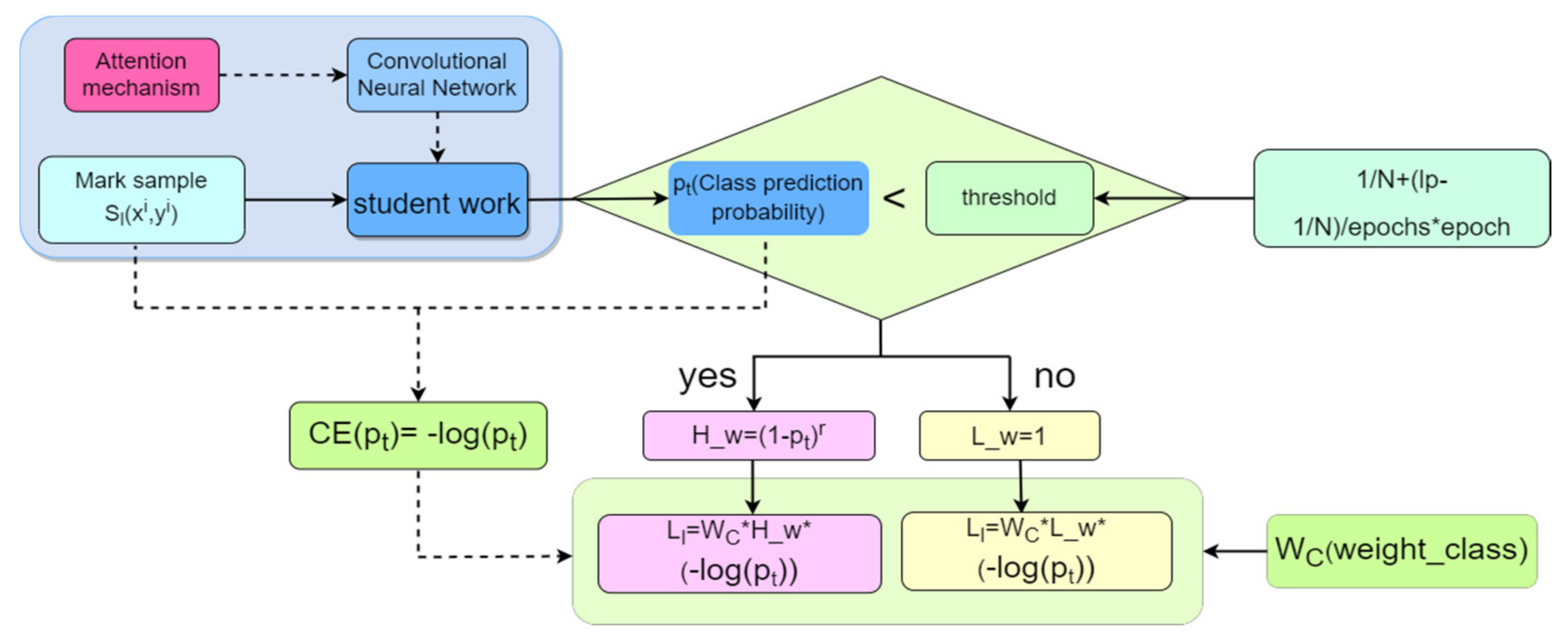
• Based on focal loss, a new loss function is introduced to supervision loss which can effectively notice samples with wrong classifications and pay more attention to the characteristics of samples that easily lead to wrong classification;
• We conduct experiments on two large medical datasets for skin lesion classification and chest diseases and the experimental results show that our model is effective and superior to the current semi-supervised learning method.

2. Related Work

This section describes some basic methods used in our proposed semi-supervised image classification framework. Specifically, Section 2.1 summarizes the previous semi-supervised models and analyzes their advantages and disadvantages. In Section 2.2 we introduce a self-attention mechanism inside the network to make it more autonomous so as to capture the features useful for the current task. Section 2.3 introduces the differences in the internal features of the samples and explores the internal semantic relations. Section 2.4 introduces the previous supervised loss function used to mark data and describes its shortcomings before introducing focal loss.

2.1. Semi-Supervised Learning Based on Consistency Regularization

The consistency-based method involves using the information of unlabeled data effectively by making two prediction results for an image consistent through random enhancement. Most previous work has tried to design an effective method to generate a consistent target close to the real mark of the image. For example, the π model directly takes the network output as the consistency target [18]. The Temporal Ensembling method [29] uses the exponential moving average (EMA) prediction result for unlabeled data as the consistency target, the quality of which can be improved because it comes from the set information of the previous period. However, the Temporal Ensembling method needs to integrate the information of the previous period, which requires a huge prediction matrix and makes training data-heavy. Therefore, the Mean Teacher [30] was brought into being. Instead of maintaining the exponential moving average (EMA) prediction, the Mean Teacher framework uses the exponential average weight of the student model to reconstruct the teacher model. Since the teacher model comes from the integration of the student model, its prediction can also produce a reliable consistency goal. Recently, some work has studied more effective image enhancement functions and how to generate more reliable consistency targets to improve the benefits of consistency regularization. For example, Xie et al. [32,33,34] proved that using better image enhancement methods to create undisturbed samples can greatly improve the performance of model classification. By enhancing the local smoothness of the given input label distribution, the proposed virtual anti-disturbance [10] can prevent the model from straying further and further from the correct path because of the bad target by generating a more reliable consistency target [35] and can improve the existing consistency-based method by exploring the internal relationships among input data [36]. Different from the above work, our goal is to effectively strengthen the performance of the classifier by paying more attention to the main characteristics of differences between different types of samples and introducing a parameter into the supervision loss to make the prediction result for each labeled sample closer to the real label.

2.2. Self-Attention Mechanism

At present, the attention mechanism [30,37,38] has been applied to various tasks in computer vision, such as image classification [38,39] and object segmentation [40]. The channel attention module [37] enhances the channel relationship by squeezing and expanding the block, thus adaptively recalibrating each channel of the current image features according to the current task and then integrating the obtained channel attention weight with the original feature map to effectively utilize some features that play a key role in the current task. Based on the channel attention mechanism, a spatial attention module [38] can be added, which can more comprehensively judge each pixel in a picture in each channel and capture them, which is relevant to the current task. Here, the channel attention module runs in series with the spatial module. Park et al. [30] proposed that the channel and spatial attention modules should be run in parallel and that the obtained channel and spatial relation matrix should be added and fused with the original feature map. In this way, the model can pay more attention to the features that play a decisive role in the current task to improve the discrimination ability of the model.

2.3. Consistency Paradigm of Sample Relationship

In the previous research work on semi-supervised learning based on consistency regularization, the features of labeled and unlabeled samples were learned as much as possible by forcing the two most different predicted values of samples through different disturbances, and no more attention was paid to the semantic relationships between samples. On the premise that human diagnosis usually makes reliable decisions based on previous cases, Liu et al. [36] introduced a novel sample relationship consistency paradigm matrix, which constructed a case-level Gram matrix to simulate the structured relationship between different samples. Given a small batch of input samples with B samples, the activation feature graph of the L layer is defined as ${\mathrm{F}}^{\mathrm{l}}\in {\mathrm{R}}^{\mathrm{B}\times \mathrm{H}\times \mathrm{W}\times \mathrm{C}}$, where H and W are the spatial dimensions of the activation feature graph, and C is the number of channels. Then, the activation feature graph is reshaped into ${\mathrm{A}}^{\mathrm{l}}\in {\mathrm{R}}^{\mathrm{B}\times \mathrm{H}\times \mathrm{W}\times \mathrm{C}}$, and its Gram matrix is calculated as follows:

$${\mathrm{G}}^{\mathrm{l}}=\left(\mathrm{A}{\left(\mathrm{xi},\mathsf{\theta },\mathsf{\eta }\right)}^{\mathrm{l}}\right)\times {\left(\mathrm{A}{\left(\mathrm{xi},\mathsf{\theta },\mathsf{\eta }\right)}^{\mathrm{l}}\right)}^{\mathrm{T}}$$

(1)

where $\mathrm{A}{\left(\mathrm{xi},\mathsf{\theta },\mathsf{\eta }\right)}^{\mathrm{l}}$ represents the activation feature graph of the layer of each sample, respectively, which means the semantic relationship of this sample in the convolutional neural network. Finally, the sample relationship matrix normalized by ${\mathrm{L}}_2$ can be defined as:

$${\mathrm{R}}^{\mathrm{l}}=\left(\frac{{\mathrm{G}}_1^{\mathrm{l}}}{\parallel {\mathrm{G}}_1^{\mathrm{l}}\parallel },\cdots \cdots ,\frac{{\mathrm{G}}_{\mathrm{B}}^{\mathrm{l}}}{\parallel {\mathrm{G}}_{\mathrm{B}}^{\mathrm{l}}\parallel }\right)$$

(2)

This encourages the model to explore additional semantic information from unlabeled data, but we think that matrix ${\mathrm{G}}^{\mathrm{l}}$ may lose some characteristic information because of its multiplication relationship and the reduction in the number of dimensions.

2.4. Supervision Loss

In recent semi-supervised classification models, the classification loss for labeled data always makes the predicted value of the sample closer to the labeled value by minimizing cross-entropy loss [39]. However, the cross-entropy function calculates the total loss of each batch in the sample, so the probability of the sample which may cause individual misjudgment approaching the real label in the later training process is low. Both focal loss [31] and reduced focal loss [40] pay more attention to misclassified samples by adding weight in front of the cross-entropy function. In the subsequent training process, they can effectively reduce the loss and make them closer to the real labels. More importantly, the performance of the classifier model will gradually improve with the training rounds. We think that the “fixation” of the weighting factor will weaken the classification effect of the model with the increase in the number of training rounds.

3. Method

Figure 1 describes our semi-supervised learning framework for medical image classification which integrates attention mechanisms and the intrinsic relationship characteristics of samples into student and teacher models. This enables the model to spontaneously capture features that are more significant in the current classification task and extract richer intrinsic information from samples of unlabeled data. Finally, the improved focus loss is introduced into the supervision loss, so that the minimization goal of the model is mainly dominated by misjudged samples, which effectively improves the performance of the model.

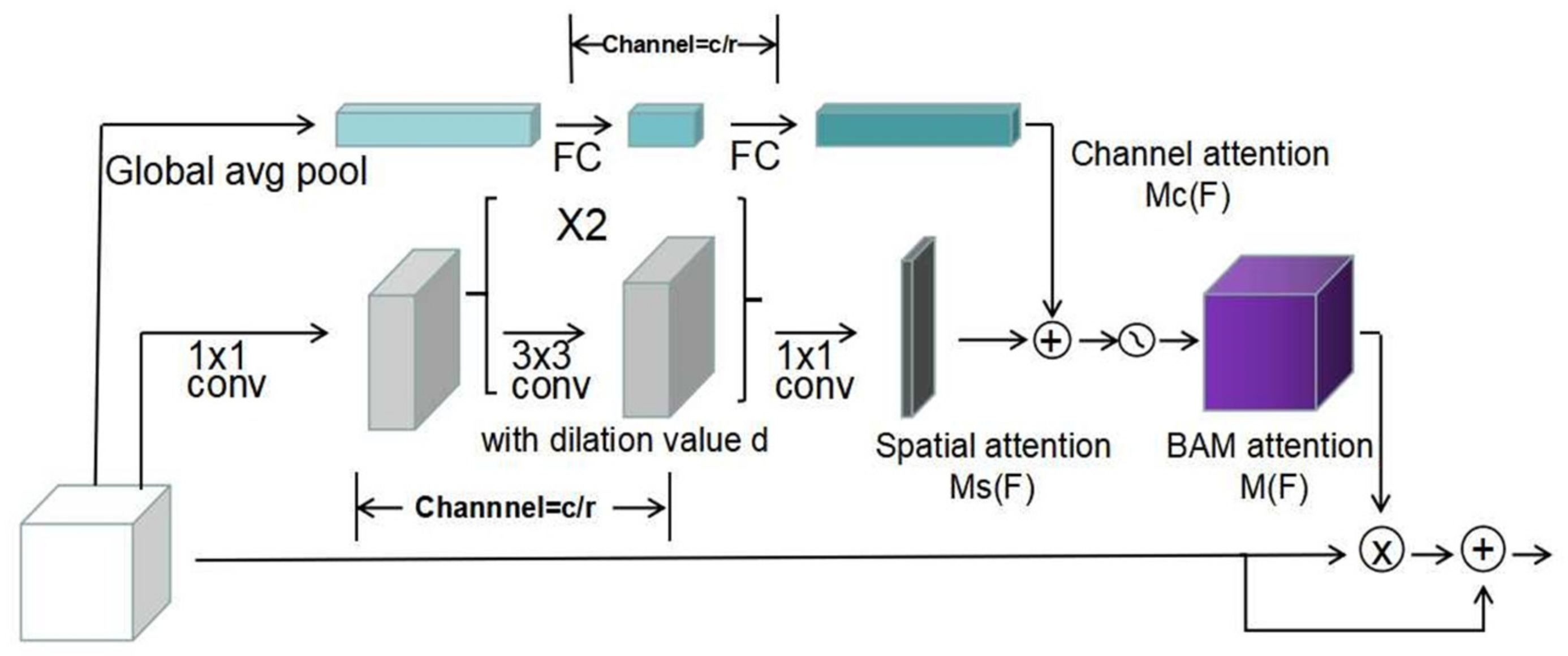
3.1. Channel and Spatial Attention Mechanisms

As depicted in Figure 2, in this paper, we add the attention mechanism proposed in [30] to the convolutional neural network, which is divided into two modules: channel attention and spatial attention. In terms of channel attention, we define the module as:

$${\mathrm{M}}_{\mathrm{c}}\left(\mathrm{F}\right)=\mathrm{BN}\left({\mathrm{W}}_1\left({\mathrm{W}}_0\mathrm{AvgPool}\left(\mathrm{F}\right){+\mathrm{b}}_0\right){+\mathrm{b}}_1\right)$$

(3)

where $\mathrm{F}\in {\mathrm{R}}^{\mathrm{H}\times \mathrm{W}\times \mathrm{C}}$ is the input image, H and W are the length and width of the input feature map, and C is the number of channels of the input feature map.${\mathrm{W}}_0\in {\mathrm{R}}^{\mathrm{C}/\mathrm{r}\times \mathrm{C}}$, ${\mathrm{b}}_0\in {\mathrm{R}}^{\mathrm{C}/\mathrm{r}}$, ${\mathrm{W}}_1\in {\mathrm{R}}^{\mathrm{C}/\mathrm{C}\times \mathrm{r}}$, ${\mathrm{b}}_1\in$ ${\mathrm{R}}^{\mathrm{C}}.$ Firstly, the input characteristic map is reshaped to $\mathrm{F}\in {\mathrm{R}}^{1\times 1\times \mathrm{C}}$ through $\mathrm{AvgPool}\left(\mathrm{F}\right)$, and then through ${\mathrm{W}}_0$ and ${\mathrm{W}}_1$, successively, the calibrated weighting matrix ${\mathrm{M}}_{\mathrm{c}}\left(\mathrm{F}\right)$ of each channel is adaptively obtained through extrusion and expansion. The spatial attention module is as follows:

$${\mathrm{M}}_{\mathrm{s}}\left(\mathrm{F}\right)=\left({\mathrm{f}}_3^{1\times 1}\left({\mathrm{f}}_2^{3\times 3}\left({\mathrm{f}}_1^{3\times 3}\left({\mathrm{f}}_0^{1\times 1}\left(\mathrm{F}\right)\right)\right)\right)\right)$$

(4)

At first, the input sample $\mathrm{F}\in {\mathrm{R}}^{\mathrm{H}\times \mathrm{W}\times \mathrm{C}}$ is subjected to a 1 × 1 convolution for dimension reduction, then two 3 × 3 cavity convolutions to increase its receptive field, and, finally, a 1 × 1 convolution is performed to obtain the weighting matrix ${\mathrm{M}}_{\mathrm{s}}\left(\mathrm{F}\right)$ of each pixel of each image in the calibrated channel. These are combined to generate the final attention feature map.

$$\mathrm{M}\left(\mathrm{F}\right)=\mathsf{\sigma }\left({\mathrm{M}}_{\mathrm{c}}\left(\mathrm{F}\right){+\mathrm{M}}_{\mathrm{s}}\left(\mathrm{F}\right)\right)$$

(5)

Since the two dimensions are different, they need to be adjusted to ${\mathrm{R}}^{\mathrm{H}\times \mathrm{W}\times \mathrm{C}}$ first. The final characteristic diagram is as follows:

$$\mathrm{F}=\left(\mathrm{F}+\mathrm{F} \times \mathrm{M}\left(\mathrm{F}\right)\right)$$

(6)

The intrinsic feature channel hides the basic information of the convolution filter, which is helpful for the network model to learn more useful features for the current task.

3.2. Loss of Consistency of Intrinsic Characteristics

Inspired by the paradigm matrix of sample relation, which encourages the network to explore the semantic relationship between unlabeled samples to improve the expressive ability of the model, the activated feature graph from the deep layer contains more advanced semantic information than the activated feature graph from the middle. As shown in Figure 1, we use the intrinsic sample features before the classification level to construct an intrinsic relationship consistency loss similar to the unsupervised loss. Given a small batch of input samples containing B samples, we define the intrinsic feature graph before the classification level as ${\mathrm{F}}^{\mathrm{l}}\in {\mathrm{R}}^{\mathrm{B}\times 1\times 1\times \mathrm{C}}$, where 1 and 1 are the spatial dimensions of the active feature graph and C is the number of channels. After the intrinsic characteristics of the student model are standardized, the matrix is as follows:

$${\mathrm{K}}_{\mathrm{l}}=\left(\frac{\mathrm{F}{\left(\mathrm{xi},\mathsf{\theta },\mathsf{\eta }\right)}_1^{\mathrm{l}}}{\parallel \mathrm{F}{\left(\mathrm{xi},\mathsf{\theta },\mathsf{\eta }\right)}_1^{\mathrm{l}}\parallel },\cdots ,\frac{\mathrm{F}{\left(\mathrm{xi},\mathsf{\theta },\mathsf{\eta }\right)}_{\mathrm{B}}^{\mathrm{l}}}{\parallel \mathrm{F}{\left(\mathrm{xi},\mathsf{\theta },\mathsf{\eta }\right)}_{\mathrm{B}}^{\mathrm{l}}\parallel }\right)$$

(7)

Similarly, after the intrinsic characteristics of the teacher model are standardized, the matrix is:

$${\mathrm{K}}_{\mathrm{l}}^{\prime }=\left(\frac{\mathrm{F}{\left({\mathrm{xi},\mathsf{\theta }}^{\prime }{,\mathsf{\eta }}^{\prime }\right)}_1^{\mathrm{l}}}{\parallel \mathrm{F}{\left({\mathrm{xi},\mathsf{\theta }}^{\prime }{,\mathsf{\eta }}^{\prime }\right)}_1^{\mathrm{l}}\parallel },\cdots ,\frac{\mathrm{F}{\left({\mathrm{xi},\mathsf{\theta }}^{\prime }{,\mathsf{\eta }}^{\prime }\right)}_{\mathrm{B}}^{\mathrm{l}}}{\parallel \mathrm{F}{\left({\mathrm{xi},\mathsf{\theta }}^{\prime }{,\mathsf{\eta }}^{\prime }\right)}_{\mathrm{B}}^{\mathrm{l}}\parallel }\right)$$

(8)

where $\mathrm{F}{\left(\mathrm{xi},\mathsf{\theta },\mathsf{\eta }\right)}^{\mathrm{l}}$ represents the intrinsic characteristic diagram of each sample, which means the internal relationship of this sample in the convolutional neural network, and the intrinsic characteristic relation matrix requires that the internal relationship characteristics of the same sample should be consistent under different disturbances. Therefore, the loss function of the sample intrinsic relationship matrix is defined as:

$${\mathrm{L}}_{\mathrm{ifr}}={{\displaystyle \sum }}_{\mathrm{x}\in \left\{{\mathrm{S}}_{\mathrm{L}}{,\mathrm{S}}_{\mathrm{U}}\right\}}\frac{1}{\mathrm{B}} \parallel {\mathrm{K}}_{\mathrm{l}}^{\prime }{-\mathrm{K}}_{\mathrm{l}}{\parallel }_2^2$$

(9)

where x is the total set of labeled and unlabeled samples, while ${\mathrm{K}}_{\mathrm{l}}^{\prime }$ and ${\mathrm{K}}_{\mathrm{l}}$ represent the intrinsic characteristic matrix of samples obtained under different weights and disturbances, respectively. By minimizing the loss function model of the intrinsic characteristic matrix of samples, it will be encouraged to capture the intrinsic differentiation characteristics among samples under different weights and disturbances and then help to obtain additional intrinsic information from unlabeled samples. In comparison, the feature map from the deep layer contains more advanced information than that from the middle. Therefore, the characteristic map before the last average pool layer is used to calculate the intrinsic characteristic matrix ${\mathrm{K}}_{\mathrm{l}}$ of the sample.

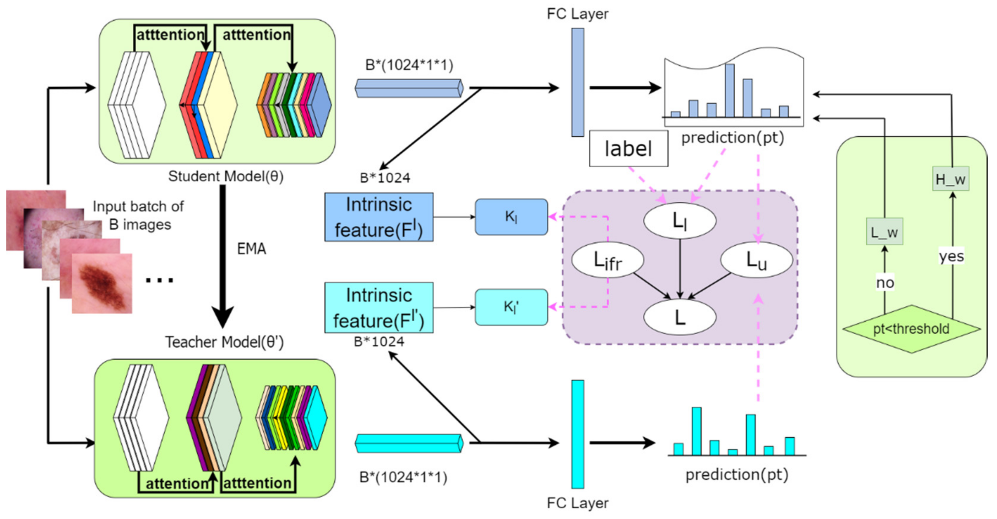
3.3. Semi-Supervised Learning Framework

The semi-supervised loss function [18,30] previously used for classification tasks can be divided into two parts: the supervised loss of labeled samples and the unsupervised consistency loss of total samples. We express labeled datasets and unlabeled datasets as ${\mathrm{S}}_{\mathrm{L}}={\left\{\left({\mathrm{x}}^{\mathrm{i}},{\mathrm{y}}^{\mathrm{i}}\right)\right\}}_{\mathrm{i}=1}^{\mathrm{N}}$ and ${\mathrm{S}}_{\mathrm{U}}={\left\{{\mathrm{x}}^{\mathrm{i}}\right\}}_{\mathrm{i}=\mathrm{N}+1}^{\mathrm{N}+\mathrm{M}}$, respectively, where ${\mathrm{x}}^{\mathrm{i}}$ is an inputted two-dimensional medical image, such as a skin lesion image or a chest disease image, and ${\mathrm{y}}^{\mathrm{i}}$ is an artificially marked image real label using one-hot coding. The overall optimization objectives of the whole framework are as follows:

$$\underset{\mathsf{\theta }}{\min }\left({{\displaystyle \sum }}_{\mathrm{i}=1}^{\mathrm{N}}{\mathrm{L}}_{\mathrm{S}}\left(\mathrm{f}\left({\mathrm{x}}_{\mathrm{i}};\mathsf{\theta }\right){,\mathrm{y}}_{\mathrm{i}}\right){+\mathsf{\lambda }\mathrm{L}}_{\mathrm{U}}\left({\left\{{\mathrm{x}}^{\mathrm{i}}\right\}}_{\mathrm{i}=\mathrm{N}+1}^{\mathrm{N}+\mathrm{M}};\mathrm{f}\left(·\right){,\mathsf{\theta },\mathsf{\eta },\mathsf{\theta }}^{\prime }{,\mathsf{\eta }}^{\prime }\right)\right)$$

(10)

where ${\mathrm{L}}_{\mathrm{S}}$ represents the supervised loss (cross-entropy loss) of labeled samples, ${\mathrm{L}}_{\mathrm{U}}$ represents the unsupervised consistency loss of total samples, $\mathrm{f}\left(·\right)$ represents the classification network, $\mathsf{\theta }$ and ${\mathsf{\theta }}^{\prime }$ are the parameter weights of the student model and teacher model, respectively, and $\mathsf{\eta }$ and ${\mathsf{\eta }}^{\prime }$, respectively, represent two different disturbances of the two models with the same input. $\mathsf{\lambda }$ is a weighting factor used to weigh the supervised loss against the unsupervised loss. Its teacher model parameter weight ${\mathsf{\theta }}^{\prime }$ is the exponential average of the student model weight $\mathsf{\theta }$, and the iterative training of teacher model weight with time is defined as:

$${\mathsf{\theta }}_{\mathrm{t}}^{\prime }{=\mathrm{a}\mathsf{\theta }}_{\mathrm{t}-1}^{\prime }+\left(1-\mathrm{a}\right){\mathsf{\theta }}_{\mathrm{t}}$$

(11)

where $\mathrm{a}$ is the smoothing coefficient super-parameter that controls the weight update rate. In terms of unsupervised loss, to encourage the consistency of the outputs of the student model and the teacher model, we keep the traditional individual consistency mechanism [29] as follows:

$${\mathrm{L}}_{\mathrm{u}}={{\displaystyle \sum }}_{\mathrm{i}=1}^{\mathrm{N}+\mathrm{M}}{\mathrm{E}}_{\mathsf{\eta },{\mathsf{\eta }}^{\prime }}\parallel \mathrm{f}\left({\mathrm{x}}_{\mathrm{i}}{,\mathsf{\theta }}^{\prime }{,\mathsf{\eta }}^{\prime }\right)-\mathrm{f}\left({\mathrm{x}}_{\mathrm{i}},\mathsf{\theta },\mathsf{\eta }\right){\parallel }_2^2$$

(12)

In terms of supervision loss, focal loss [31] is defined as follows:

$$\mathrm{FL}\left({\mathrm{p}}_{\mathrm{t}}\right)=-{\left(1-{\mathrm{p}}_{\mathrm{t}}\right)}^{\mathsf{\gamma }}\log \left({\mathrm{p}}_{\mathrm{t}}\right)$$

(13)

${\mathrm{p}}_{\mathrm{t}}$ is set to:

$${\mathrm{p}}_{\mathrm{t}}=\left\{\begin{array}{cc}\mathrm{p}& \mathrm{if} \mathrm{y}=1\\ 1-\mathrm{p}& \mathrm{otherwise}\end{array}\right.$$

(14)

${\mathrm{p}}_{\mathrm{t}}$ marks the predicted probability value of the sample. In Figure 3, we introduce the super-parameter threshold on the basis of focal loss. Compared with this, the supervision loss is defined as follows:

$${\mathrm{L}}_{\mathrm{l}}=\left\{\begin{array}{cc}{\mathrm{W}}_{\mathrm{C}} \times \mathrm{L}\_\mathrm{w} \times (-\log \left({\mathrm{p}}_{\mathrm{t}}\right))& \mathrm{otherwise}\\ {\mathrm{W}}_{\mathrm{C}} \times \mathrm{H}\_\mathrm{w} \times (-\log \left({\mathrm{p}}_{\mathrm{t}}\right))& \mathrm{if} {\mathrm{p}}_{\mathrm{t}}>\mathrm{threshold}\end{array}\right.$$

(15)

where $\mathrm{L}\_\mathrm{w}=1$ and $\mathrm{H}\_\mathrm{w}={\left(1-{\mathrm{p}}_{\mathrm{t}}\right)}^{\mathsf{\gamma }}$, respectively, represent the weights that should be given to the samples with wrong classification and correct classification. As the number of training rounds increases, the classification performance of the model will be continuously improved and the value of ${\mathrm{p}}_{\mathrm{t}}$ will also increase (it will not exceed the predicted value of 1), so we set the threshold as follows:

$$\mathrm{threshold}=\left(1/\mathrm{N}\right)+\left(\mathrm{lp}-\frac{1}{\mathrm{N}}\right)/\mathrm{epochs} \times \mathrm{epoch}$$

(16)

Since the categories of datasets are unbalanced, ${\mathrm{W}}_{\mathrm{C}}$ is the weight of each category in the total sample, while the tag predicts that the sum of each category is 1, $\mathrm{N}$ is the total number of categories of datasets, epochs is the total number of training rounds, and epoch is the current round.

3.4. Total Loss Function and Details

Our semi-supervised learning framework is based on the consistent regularization machine strategy [18], that is, two predicted values obtained by forcing the same samples to be similar in two random enhancement ways are used as labeled data. Finally, the overall optimization loss function of the whole framework can be described as follows:

$${\mathrm{L}=\mathrm{L}}_{\mathrm{l}}+\mathsf{\lambda }\left({\mathrm{L}}_{\mathrm{u}}{+\mathrm{L}}_{\mathrm{ifr}}\right)$$

(17)

In the formula, the former item is the supervised loss of marked samples, and the latter item is the unsupervised loss, which is a super-parameter to balance the supervised loss and unsupervised loss.

For comparison with the original paper, during the training period, we adopted the same image enhancement technology and set a series of parameters. For example, we adopted two random perturbation forms, including (1) image enhancement, random rotation, translation, horizontal flipping, etc., to randomly transform each sample in each small batch. At the same time, the rotation angle was in the range of −10 to 10, the horizontally and vertically translated pixels ranged from −2% to 2% of the image width, and the input was randomly flipped horizontally and vertically with a probability of 50%. (2) Dropout layer in the network: we added a random dropout layer before the last pool layer in each block of the densenet network [41] that we used, with a dropout rate of 0.2, which is only turned on in the training stage and is turned off in the verification and testing stages.

4. Experiments

In this section, we describe some experiments with two large public medical datasets, namely, the ISIC 2018 skin lesions dataset (single label) and the ChestX-ray14 chest diseases dataset (multi-label), and then discuss the experimental results to evaluate our proposed method.

4.1. Parameter Setting

As the following parameters have been mentioned in the previous model, for comparison with the original paper [36], we improve and recast our model based on SRC-MT common code and implement our method with densenet as the backbone of the network, which is trained by the Adam optimizer [42] with default parameter settings. We set the batch size to 48, and each small batch contains 12 labeled samples and 36 unlabeled samples. In Equation (3), the parameter r is set to 16 [30] and the self-attention module is placed in the pool layer behind each block of the network [30]. In Equation (11), the exponential average attenuation rate a is set to 0.99, just as mentioned in [28,29]. γ in Equation (15) is set to 2, and we imagine the trained classifier as the ideal situation. We set $\mathrm{l}\mathrm{p}$ in Equation (16) to 1 and we define $\mathsf{\lambda }$ in Equation (17) as:

$${\mathsf{\lambda }}_{\mathrm{t}}{=1 \times \mathrm{e}}^{{\left(-5\left(1-\mathrm{t}/\mathrm{T}\right)\right)}^2}$$

(18)

This is used to control the value of λ, to ensure that the training loss will not be dominated by the unsupervised loss at the beginning of network training when the consistency target of labeled data is unreliable [10]. The learning rate is initialized to ${\mathrm{e}}^{-4}$ and decays exponentially with the power of 0.9 after each round.

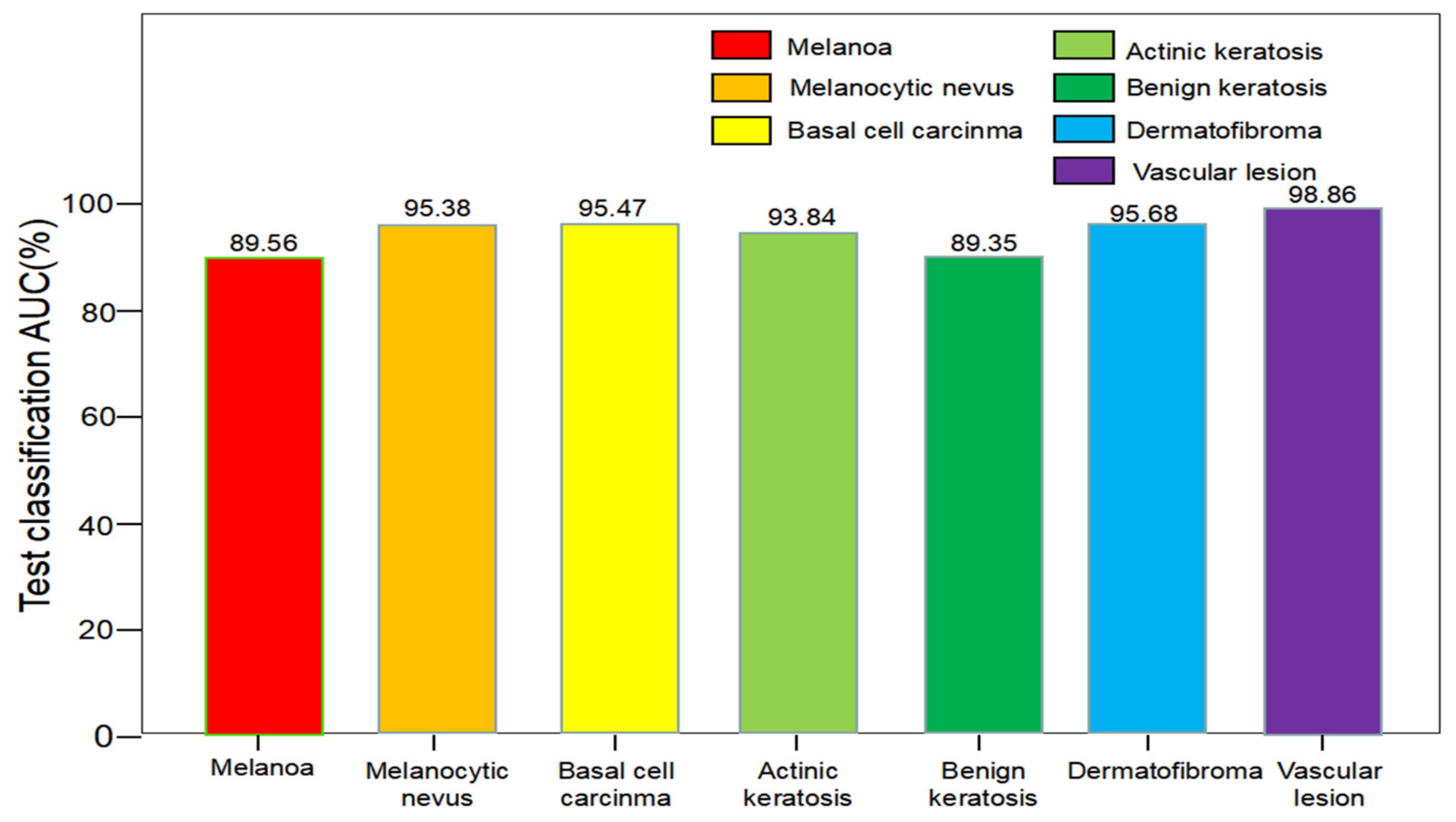
4.2. ISIC 2018 Dataset

The ISIC 2018 dataset is used for single-label classification. It consists of 10,015 skin lesion examination images, which are labeled as instances of seven common skin lesions. We divide the dataset as follows: 70% for training, 10% for verification, and 20% for testing. There are 60 rounds of training, and the ramp factor T is set to 30. Before training, we adjust each image in the dataset to a size of 224 × 224 and normalize it using the statistical data collected from the ImageNet dataset. We use DenseNet121 [4], which is pre-trained on ImageNet, as the backbone of our network, and use AUC—Accuracy, Sensitivity, and Specificity—to evaluate our model.

Table 1. Performance comparison between the ISIC 2018 dataset and previous examples of semi-supervised learning.

Method	Metrics
	AUC	Sensitivity	Accuracy	Specificity
Self-training [8]	90.58	67.63	92.37	93.31
SS-DCGAN [14]	91.28	67.72	92.27	92.56
TCSE [17]	92.24	68.17	92.35	92.51
TE [30]	92.70	69.81	92.26	92.55
MT [18]	92.96	69.75	92.48	92.20
SRC-MT [39]	93.58	71.47	92.54	92.72
Ours	94.02	72.03	92.61	91.78

shows the classification performance of the latest semi-supervised framework with 20% of the labeled data (1400 images). As we can see, the self-training method has more advantages than other methods in terms of Specificity, while its indicators need to be improved. While SS-DCGAN improves AUC by 0.7%, which indicates that the GAN-based method helps to improve the semi-supervised classification framework. On the other hand, the TCSE method indexes show that consistency regularization is effective in utilizing unlabeled data. However, TE integrates the forecasts of different periods and generates a more reliable consistency target, so it performs slightly better than TCSE. The performance of MT AUC proves its superiority in semi-supervised learning. SRC-MT improves four indicators at the same time, which proves that SRC can make full use of unlabeled data information. The AUC and Sensitivity indicators for our method show that it helps the model to make more effective use of unlabeled data and improve the classification of positive samples, while the improved performance of negative samples is poor.

We also studied the influence of the different percentages of labeled data, as shown in

Table 2. Performance comparison of our methods on the ISIC 2018 dataset with different percentages of labeled data.

Method	Percentage		Metrics
	Labeled	Unlabeled	AUC	Sensitivity	Accuracy	Specificity
Upper bound	100%	0	95.43	75.20	95.10	94.94
SRC-MT	5%	95%	87.61	62.04	88.77	89.36
Ours	5%	95%	89.56	64.32	88.56	88.96
SRC-MT	10%	90%	90.31	66.29	89.30	90.47
Ours	10%	90%	91.24	67.56	89.56	90.16
SRC-MT	20%	80%	93.58	71.47	92.54	92.72
Ours	20%	80%	94.02	72.03	92.61	91.78

: under the settings of 5%, 10%, and 20% labeled data, our method achieved 94.02% AUC and 72.03% Sensitivity, but the results were not clear for the other two indicators. These results demonstrate the impact of our method with different labeling ratios for the data.

Figure 4 shows the AUC indicators of our method for each category of the ISIC 2018 dataset, in which the AUC performance of our method reaches 95% in most categories, and the worst performance in Melanoa and Benign keratosis, which may be due to the small number of inter-class characteristics making it difficult for the model to accurately identify it.

4.3. ChestX-ray14 Dataset

The ChestX-ray14 dataset is used for multi-label classification. It contains 112,120 frontal chest X-rays of 30,805 unique patients, each of which is marked with one or more common chest diseases out of a total of 14. In order to make a fair comparison with the previous methods, we divided them into a training set, a verification set, and a test set with the proportions 70%, 10%, and 20%. They were a total of 20 rounds of training, and the slope factor T was set to 10. Before training, we adjusted each image in the dataset to the size of 384 × 384 and normalized it using the statistical data collected from the ImageNet dataset. As this dataset is much larger than ISIC 2018 dataset, DenseNet169 pre-trained on ImageNet was adopted as our network backbone. Referring to the previous work [15], we only used AUC as our model evaluation index.

Table 3. AUC performance comparison of semi-supervised models with different markers on the ChestX-ray14 dataset.

Label Percentage	2%	5%	10%	15%	20%
GraphXNET [15]	53	58	63	68	78
SRC-MT	66.95	72.29	75.28	77.76	79.23
Ours	68.24	73.65	77.62	78.35	79.74

compares the performance of the previous method with ours under the different percentages of labeled data. The observation shows that GraphX^NET performs particularly well with 20% labeled data, but its fluctuations with labeled data are very large, indicating that it largely depends on the size of labeled samples. SRC-MT is not only superior to the GraphX^NET method but also more “stable” given the same scale change of labeled data. However, our method has better AUC performance than SRC-MT in each percentage marking stage, and its stability has not decreased.

Table 4. Semi-supervised model’s AUC performance with respect to different categories in the ChestXray-14 dataset.

Method	Fully Supervised	MT	SRC-MT	Ours
Labeled	100%	20%	20%	20%
Unlabeled	0	80%	80%	80%
Atelectasis	77.32	75.12	75.38	76.12
Cardiomegaly	88.85	87.37	87.70	88.06
Effusion	82.11	80.81	81.58	81.77
Infiltration	70.95	70.67	70.40	70.57
Mass	82.92	77.72	78.03	78.86
Nodule	77.00	73.27	73.64	74.23
Pneumonia	71.28	69.17	69.27	69.56
Pneumothorax	86.87	85.63	86.12	86.32
Consolidation	74.88	72.51	73.11	73.84
Edema	84.74	82.72	82.94	83.13
Emphysema	93.35	88.16	88.98	90.02
Fibrosis	84.46	78.24	79.22	80.43
Pleural Thickening	77.34	74.43	75.63	75.61
Hernia	92.51	87.74	87.27	87.86
Average AUC	81.75	78.83	79.23	79.74

compares our method with MT and SRC-MT to analyze the impact on multi-label classification tasks. As we have observed, with 20% labeled data, our method achieves 79.74% AUC, which is better than that of MT 78.83% and SRC-MT 79.23%. Among 14 kinds of chest diseases, there may be some differences among the categories due to the imbalance of sample classification, but they are generally good, which can prove the effectiveness of our proposed method for multi-label classification.

4.4. Discussion of Parameters (lp)

The parameter lp in the supervision loss indicates the prediction probability value for the model pair and each category after the training. As shown in

Table 5. Effects of different lp parameter values on the performance of our semi-supervised model on the ISIC 2018 dataset.

Parameter (lp)	Metrics
	AUC	Sensitivity	Accuracy	Specificity
0.6	92.24	68.34	91.06	89.65
0.7	92.70	69.75	91.54	90.86
0.8	93.55	71.54	91.98	91.24
0.9	93.86	71.87	92.24	91.66
1.0	94.02	72.03	92.61	91.78

, we also studied the influence of lp hyperparameters in Equation (16) in different conditions. Generally speaking, we adopted different lp values in the range of 0.6 to 1.0 and examined the performance of our network model with 20% labeled data. It can be seen that, with the lp range at 0.8, our model performance is not very sensitive to lp values, and that the larger the lp value is, the better the model’s performance. Therefore, we set the value of lp to 1 in the experiment.

5. Discussion

We conduct experiments on the ISIC 2018 dataset and the ChestX-ray14 dataset and compared them with existing semi-supervised learning methods. Specifically, the experimental results for the two datasets show that, compared with the original methods, our method has improved AUC and Sensitivity, and the AUC performance on the ChestX-ray14 dataset also proved significant. However, for the ISIC 2018 dataset, the Accuracy and Specificity results were not so ideal.

The above experimental results show that it is a good idea for us to automatically capture important features by adding a self-attention mechanism to the backbone network and to weight the supervision loss of labeled samples by exploring intrinsic feature relationships among samples and introducing super-parameters related to the performance of the classifier. However, the experimental results for Accuracy and Specificity show that our method still has shortcomings and we think that the reason for this result may be that the ISIC 2018 dataset has a small number of samples and uneven distribution of positive and negative samples. In the future, we can try to manually generate some images to rectify the imbalance of samples in the hope that we can achieve a good performance on all indicators.

In real life, many datasets may have only a small portion of labeled data, with most of the data remaining unlabeled. Existing semi-supervised models can classify these data. However, we have improved the AUC and Sensitivity metrics by improving the existing methods, and we think that our proposed loss of intrinsic feature consistency and improvement of supervisory loss are still meaningful contributions.

6. Conclusions

In the present work, we have studied the problem of semi-supervised learning in medical image classification that aims to reduce the manual labeling of medical image data. We introduced the self-attention mechanism into the backbone network to focus more on the features that are more relevant to the current task and used the improved version of focal loss to narrow the gap between wrongly classified and correctly labeled samples at the supervision loss point and recommended the intrinsic feature consistency loss of the sample to make more effective use of the unlabeled data. Compared with existing semi-supervised learning methods, our experimental results for two datasets show that our method achieved 94.02% and 72.03% on AUC and Sensitivity indicators, but its Accuracy and Specificity scores were not so good. This shows that our method still has some shortcomings, but it is worth discussing exploring the intrinsic characteristic relationships among samples and controlling the weighting of sample loss by introducing a super-parameter that varies with the performance of the classifier model. In addition, the proposed consistency loss and supervised loss functions of sample intrinsic characteristics can also be combined with other semi-supervised methods.

References

1. Krizhevsky, A.; Sutskever, I.; Hinton, G.E. Imagenet classification with deep convolutional neural networks. Adv. Neural Inf. Process. Syst. 2012, 25. [Google Scholar] [CrossRef]
2. He, K.; Zhang, X.; Ren, S.; Sun, J. Deep residual learning for image recognition. In Proceedings of the IEEE Conference on Computer Vision and Pattern Recognition, Las Vegas, NV, USA, 27–30 June 2016; pp. 770–778. [Google Scholar]
3. Ren, S.; He, K.; Girshick, R.; Sun, J. Faster r-cnn: Towards real-time object detection with region proposal networks. Adv. Neural Inf. Process. Syst. 2015, 28. [Google Scholar] [CrossRef] [Green Version]
4. Sedai, S.; Mahapatra, D.; Hewavitharanage, S.; Maetschke, S.; Garnavi, R. Semi-supervised segmentation of optic cup in retinal fundus images using variational autoencoder. In Proceedings of the International Conference on Medical Image Computing and Computer-Assisted Intervention, Quebec City, QC, Canada, 11–13 September 2017; Springer: Cham, Switzerland, 2017; pp. 75–82. [Google Scholar]
5. Su, H.; Shi, X.; Cai, J.; Yang, L. Local and global consistency regularized mean teacher for semi-supervised nuclei classification. In Proceedings of the International Conference on Medical Image Computing and Computer-Assisted Intervention, Shenzhen, China, 13–17 October 2019; Springer: Cham, Switzerland, 2019; pp. 559–567. [Google Scholar]
6. Feng, X.; Yang, J.; Laine, A.F.; Angelini, E.D. Discriminative localization in CNNs for weakly-supervised segmentation of pulmonary nodules. In Proceedings of the International Conference on Medical Image Computing and Computer-Assisted Intervention, Quebec City, QC, Canada, 11–13 September 2017; Springer: Cham, Switzerland, 2017; pp. 568–576. [Google Scholar]
7. Kamnitsas, K.; Baumgartner, C.; Ledig, C.; Newcombe, V.; Simpson, J.; Kane, A.; Menon, D.; Nori, A.; Criminisi, A.; Rueckert, D.; et al. Unsupervised domain adaptation in brain lesion segmentation with adversarial networks. In Proceedings of the International Conference on Information Processing in Medical Imaging, Boone, NC, USA, 25–30 June 2017; Springer: Cham, Switzerland, 2017; pp. 597–609. [Google Scholar]
8. Bai, W.; Oktay, O.; Sinclair, M.; Suzuki, H.; Rajchl, M.; Tarroni, G.; Glocker, B.; King, A.; Matthews, P.M.; Rueckert, D. Semi-supervised learning for network-based cardiac MR image segmentation. In Proceedings of the International Conference on Medical Image Computing and Computer-Assisted Intervention, Quebec City, QC, Canada, 11–13 September 2017; Springer: Cham, Switzerland, 2017; pp. 253–260. [Google Scholar]
9. Jin, Y.; Cheng, K.; Dou, Q.; Heng, P.A. Incorporating temporal prior from motion flow for instrument segmentation in minimally invasive surgery video. In Proceedings of the International Conference on Medical Image Computing and Computer-Assisted Intervention, Shenzhen, China, 13–17 October 2019; Springer: Cham, Switzerland, 2019; pp. 440–448. [Google Scholar]
10. Miyato, T.; Maeda, S.; Koyama, M.; Ishii, S. Virtual adversarial training: A regularization method for supervised and semi-supervised learning. IEEE Trans. Pattern Anal. Mach. Intell. 2018, 41, 1979–1993. [Google Scholar] [CrossRef] [Green Version]
11. Chartsias, A.; Joyce, T.; Papanastasiou, G.; Semple, S.; Williams, M.; Newby, D.; Dharmakumar, R.; Tsaftaris, S.A. Factorised spatial representation learning: Application in semi-supervised myocardial segmentation. In Proceedings of the International Conference on Medical Image Computing and Computer-Assisted Intervention, Strasbourg, France, 16–20 September 2018; Springer: Cham, Switzerland, 2018; pp. 490–498. [Google Scholar]
12. Nie, D.; Gao, Y.; Wang, L.; Shen, D. ASDNet: Attention based semi-supervised deep networks for medical image segmentation. In Proceedings of the International Conference on Medical Image Computing and Computer-Assisted Intervention, Strasbourg, France, 16–20 September 2018; Springer: Cham, Switzerland, 2018; pp. 370–378. [Google Scholar]
13. Dong, N.; Kampffmeyer, M.; Liang, X.; Wang, Z.; Dai, W.; Xing, E. Unsupervised domain adaptation for automatic estimation of cardiothoracic ratio. In Proceedings of the International Conference on Medical Image Computing and Computer-Assisted Intervention, Strasbourg, France, 16–20 September 2018; Springer: Cham, Switzerland, 2018; pp. 544–552. [Google Scholar]
14. Diaz-Pinto, A.; Colomer, A.; Naranjo, V.; Morales, S.; Xu, Y.; Frangi, A.F. Retinal image synthesis and semi-supervised learning for glaucoma assessment. IEEE Trans. Med. Imaging 2019, 38, 2211–2218. [Google Scholar] [CrossRef]
15. Aviles-Rivero, A.I.; Papadakis, N.; Li, R.; Sellars, P.; Fan, Q.; Tan, R.T.; Schönlieb, C.B. GraphXNET—Chest X-Ray Classification under Extreme Minimal Supervision. In Proceedings of the International Conference on Medical Image Computing and Computer-Assisted Intervention, Shenzhen, China, 13–17 October 2019; Springer: Cham, Switzerland, 2019; pp. 504–512. [Google Scholar]
16. Li, X.; Yu, L.; Chen, H.; Fu, C.-W.; Xing, L.; Heng, P.-A. Transformation-consistent self-ensembling model for semisupervised medical image segmentation. IEEE Trans. Neural Netw. Learn. Syst. 2020, 32, 523–534. [Google Scholar] [CrossRef]
17. Li, X.; Yu, L.; Chen, H.; Fu, C.W.; Heng, P.A. Semi-supervised skin lesion segmentation via transformation consistent self-ensembling model. arXiv 2018, arXiv:1808.03887. [Google Scholar]
18. Laine, S.; Aila, T. Temporal ensembling for semi-supervised learning. arXiv 2016, arXiv:1610.02242. [Google Scholar]
19. Cui, W.; Liu, Y.; Li, Y.; Guo, M.; Li, Y.; Li, X.; Wang, T.; Zeng, X.; Ye, C. Semi-supervised brain lesion segmentation with an adapted mean teacher model. In Proceedings of the International Conference on Information Processing in Medical Imaging, Hong Kong, China, 2–7 June 2019; Springer: Cham, Switzerland, 2019; pp. 554–565. [Google Scholar]
20. Yu, L.; Wang, S.; Li, X.; Fu, C.W.; Heng, P.A. Uncertainty-aware self-ensembling model for semi-supervised 3D left atrium segmentation. In Proceedings of the International Conference on Medical Image Computing and Computer-Assisted Intervention, Shenzhen, China, 13–17 October 2019; Springer: Cham, Switzerland, 2019; pp. 605–613. [Google Scholar]
21. Codella NC, F.; Nguyen, Q.B.; Pankanti, S.; Gutman, D.A.; Helba, B.; Halpern, A.C.; Smith, J.R. Deep learning ensembles for melanoma recognition in dermoscopy images. IBM J. Res. Dev. 2017, 61, 5:1–5:15. [Google Scholar] [CrossRef] [Green Version]
22. Yu, L.; Chen, H.; Dou, Q.; Qin, J.; Heng, P.-A. Automated melanoma recognition in dermoscopy images via very deep residual networks. IEEE Trans. Med. Imaging 2016, 36, 994–1004. [Google Scholar] [CrossRef]
23. Zhang, J.; Xie, Y.; Xia, Y.; Shen, C. Attention residual learning for skin lesion classification. IEEE Trans. Med. Imaging 2019, 38, 2092–2103. [Google Scholar] [CrossRef]
24. Wang, X.; Peng, Y.; Lu, L.; Lu, Z.; Bagheri, M.; Summers, R.M. Chestx-ray8: Hospital-scale chest x-ray database and benchmarks on weakly-supervised classification and localization of common thorax diseases. In Proceedings of the IEEE Conference on Computer Vision and Pattern Recognition, Honolulu, HI, USA, 21–26 July 2017; pp. 2097–2106. [Google Scholar]
25. Ganster, H.; Pinz, P.; Rohrer, R.; Wildling, E.; Binder, M.; Kittler, H. Automated melanoma recognition. IEEE Trans. Med. Imaging 2001, 20, 233–239. [Google Scholar] [CrossRef]
26. Irvin, J.; Rajpurkar, P.; Ko, M.; Yu, Y.; Ciurea-Ilcus, S.; Chute, C.; Marklund, H.; Haghgoo, B.; Ball, R.; Shpanskaya, K.; et al. Chexpert: A large chest radiograph dataset with uncertainty labels and expert comparison. In Proceedings of the AAAI Conference on Artificial Intelligence, Honolulu, HI, USA, 27 January–1 February 2019; Volume 33, pp. 590–597. [Google Scholar]
27. Rajpurkar, P.; Irvin, J.; Zhu, K.; Yang, B.; Mehta, H.; Duan, T.; Ding, D.; Bagul, A.; Langlotz, C.; Shpanskaya, K.; et al. Chexnet: Radiologist-level pneumonia detection on chest x-rays with deep learning. arXiv 2017, arXiv:1711.05225. [Google Scholar]
28. Aviles-Rivero, A.I.; Papadakis, N.; Li, R.; Sellars, P.; Alsaleh, S.M.; Tan, R.T.; Schönlieb, C.-B. Energy Models for Better Pseudo-Labels: Improving Semi-Supervised Classification with the 1-Laplacian Graph Energy. arXiv 2019, arXiv:1906.08635. [Google Scholar]
29. Tarvainen, A.; Valpola, H. Mean teachers are better role models: Weight-averaged consistency targets improve semi-supervised deep learning results. Adv. Neural Inf. Process. Syst. 2017, 30. [Google Scholar]
30. Park, J.; Woo, S.; Lee, J.Y.; Kweon, I.S. Bam: Bottleneck attention module. arXiv 2018, arXiv:1807.06514. [Google Scholar]
31. Lin, T.Y.; Goyal, P.; Girshick, R.; He, K.; Dollar, P. Focal loss for dense object detection. In Proceedings of the IEEE International Conference on Computer Vision, Venice, Italy, 22–29 October 2017; pp. 2980–2988. [Google Scholar]
32. Xie, Y.; Zhang, J.; Xia, Y. Semi-supervised adversarial model for benign–malignant lung nodule classification on chest CT. Med. Image Anal. 2019, 57, 237–248. [Google Scholar] [CrossRef]
33. Yun, S.; Han, D.; Oh, S.J.; Chun, S.; Choe, J.; Yoo, Y. Cutmix: Regularization strategy to train strong classifiers with localizable features. In Proceedings of the IEEE/CVF International Conference on Computer Vision, Seoul, Korea, 27 October–2 November 2019; pp. 6023–6032. [Google Scholar]
34. French, G.; Oliver, A.; Salimans, T. Milking cowmask for semi-supervised image classification. arXiv 2020, arXiv:2003.12022. [Google Scholar]
35. Liu, L.; Tan, R.T. Certainty driven consistency loss on multi-teacher networks for semi-supervised learning. Pattern Recognit. 2021, 120, 108140. [Google Scholar] [CrossRef]
36. Liu, Q.; Yu, L.; Luo, L.; Dou, Q.; Heng, P.A. Semi-supervised medical image classification with relation-driven self-ensembling model. IEEE Trans. Med. Imaging 2020, 39, 3429–3440. [Google Scholar] [CrossRef]
37. Hu, J.; Shen, L.; Sun, G. Squeeze-and-excitation networks. In Proceedings of the IEEE Conference on Computer Vision and Pattern Recognition, Salt Lake City, UT, USA, 18–22 June 2018; pp. 7132–7141. [Google Scholar]
38. Woo, S.; Park, J.; Lee, J.Y.; Kweon, S. Cbam: Convolutional block attention module. In Proceedings of the European Conference on Computer Vision (ECCV), Munich, Germany, 8–14 September 2018; pp. 3–19. [Google Scholar]
39. De Boer, P.T.; Kroese, D.P.; Mannor, S.; Rubinstein, R.Y. A tutorial on the cross-entropy method. Ann. Oper. Res. 2005, 134, 19–67. [Google Scholar] [CrossRef]
40. Sergievskiy, N.; Ponamarev, A. Reduced focal loss: 1st place solution to xview object detection in satellite imagery. arXiv 2019, arXiv:1903.01347. [Google Scholar]
41. Huang, G.; Liu, Z.; Van Der Maaten, L.; Weinberger, K.Q. Densely connected convolutional networks. In Proceedings of the IEEE Conference on Computer Vision and Pattern Recognition, Honolulu, HI, USA, 21–26 July 2017; pp. 4700–4708. [Google Scholar]
42. Kingma, D.P.; Ba, J. Adam: A method for stochastic optimization. arXiv 2014, arXiv:1412.6980. [Google Scholar]
Figure 1. Overview of our semi-supervised framework for medical image classification. The teacher’s weight θ is updated to the exponential moving average (EMA) of the student’s weight θ . The objective function of optimizing the student model includes the supervised loss ( L l ) on the marked set and two unsupervised consistency losses ( L ifr and L u ) on the unlabeled set and the marked set, respectively. By minimizing the three losses, the whole framework can fully mine the features of labeled samples and unlabeled ones, thereby accurately classifying them.
Applsci 12 06726 g001
Figure 2. The attention module structure of this paper consists of two modules: channel attention and spatial attention. The two modules run in parallel, and the weighed matrixes of each channel of the sample features and of each image pixel in the channel are obtained spontaneously and then integrated into the original sample features.
Applsci 12 06726 g002
Figure 3. A detailed description of our semi-supervised framework supervision loss.
Applsci 12 06726 g003
Figure 4. AUC performance of each category for the ISIC 2018 dataset.
Applsci 12 06726 g004