1. Introduction
Cancer is a serious health issue around the world. It is the second leading cause of death, following cardiovascular diseases [
1]. Among the various kinds of cancer, brain tumors (BTs) are a life-threatening type due to their heterogeneous features, aggressive nature, and small survival rate. BTs are classified into distinct types based on their texture, location, and shape [
2]. Based on the type of tumor, physicians can predict and diagnose patient endurance and make decisions regarding the right treatment, which could range from surgery, succeeded by chemotherapy and then radiotherapy, to playing a waiting game method that ignores invading processes. Therefore, tumor grading is a significant factor in treatment monitoring and planning [
3,
4].
Magnetic Resonance Imaging (MRI) is a non-invasive, pain-free medical imaging process that utilizes high-quality images of human body organs in 3D and 2D formats [
5]. It is extensively utilized because it is the most precise method for categorizing and identifying cancer, owing to its high-resolution images of the brain tissues [
6,
7]. However, identifying the cancer variety with MRI images is difficult and prone to error. In particular, the accuracy is based on the experience of the radiologist, and it is significant to note that it is a time-consuming process [
8]. Additionally, accurate analysis aids the patient in initiating the right treatment promptly and living a longer life [
9]. This creates a high demand in the Artificial Intelligence (AI) domain for developing and designing a novel and creative Computer Assisted Diagnosis (CAD) process that focuses on easing the work pressure of the analysis and categorization of tumors and functions as a useful tool for radiologists and doctors [
10].
CAD methods are useful for neuro-oncologists in various aspects. CAD methods pave the way in the classification and early detection of BTs [
11]. Doctors, with the help of CAD, can perform highly precise categorizations compared to those dependent on visual comparisons. MRIs contain useful data about the position, shape, type, and size of BTs and do not expose the patient to dangerous ionizing radiation. MRIs offer high contrast of soft tissues compared to computerized tomography (CT) scans. Therefore, joined with the CAD model, MRIs may help rapidly identify tumors’ size and location. Developments in computers have designed strong tools which can help to attain more precise diagnoses. These developments in deep learning-related systems have led to a massive enhancement in medical image analysis and decision making. Particularly deep neural network (DNN)-related technologies utilized by well-trained experts [
12].
Due to the rapid advancement of deep learning (DL) methods and their capability to classify medical images in a better way, CAD is a widely used methodology of diagnosis among medical imaging experts. Expanding research in applying DL to the categorization of multiple diseases within the limitations of existing technologies is presently a leading focus of radiology research scholars. Of the multitude of deep machine learning (ML) methods, CNNs are widely utilized for the medical image examination of distinct diseases and, thus, extensively used by researchers.
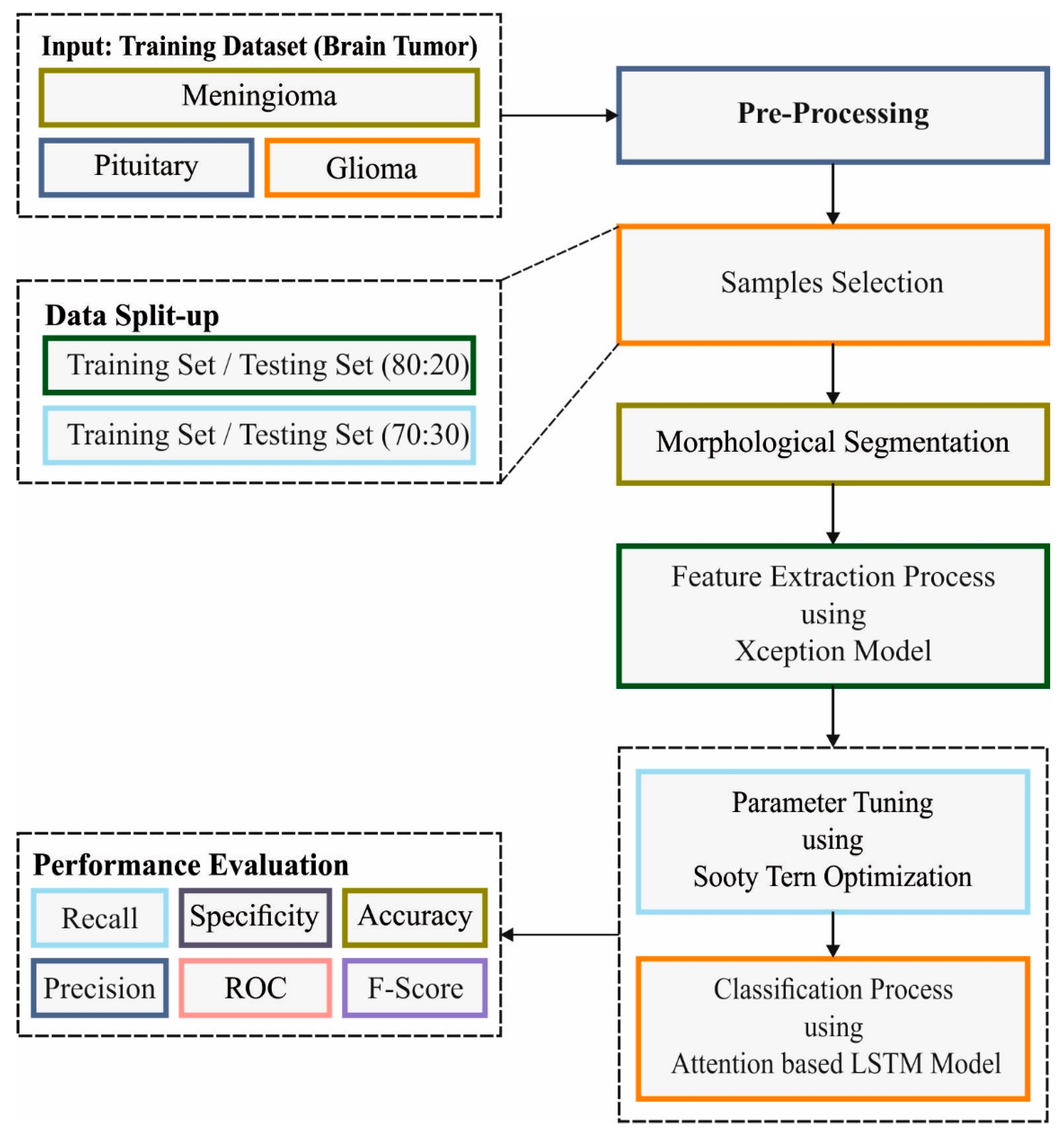
This study designs an evolutional algorithm with a deep learning-driven brain tumor MRI image classification (EADL-BTMIC) model. The presented EADL-BTMIC model applies bilateral filtering (BF) based noise removal and skull stripping as a pre-processing stage. Additionally, the morphological segmentation process is carried out to determine the affected regions in the image. In addition, sooty tern optimization (STO) with the Xception model is exploited for feature extraction purposes. Finally, the attention-based long short-term memory (ALSTM) technique is exploited for classifying BT into distinct classes. A detailed experimental analysis is carried out to examine the performance of the EADL-BTMIC model. In short, this paper’s contribution is summarized as follows:
An intelligent EADL-BTMIC model comprising pre-processing, morphological segmentation, Xception-based feature extraction, STO parameter tuning, and ALSTM classification using MRI images is presented. To the best of our knowledge, the EADL-BTMIC model has never been presented in the literature.
A novel STO algorithm with the Xception model is applied for the hyperparameter tuning process, which helps in boosting the overall BT classification performance.
2. Related Works
The authors in [
13] developed a BT classification method based on the hybrid brain tumor classification (HBTC) model. The presented model reduces the intrinsic difficulties and enhances the classification performance. Additionally, many ML models such as multilayer perception (MLP), J48, meta bagging (MB), and random tree (RT) are used for the classification of cyst, glioma, menin, and meta tumors. The authors in [
14] presented a multi-level attention model to classify BT. The presented multi-level attention network (MANet) comprises spatial and cross-channel attention that concentrates on tumor region prioritization and manages cross-channel temporal dependency existing in the semantic feature sequence attained from the Xception backbone. Nayak et al. [
15] presented a CNN-based dense EfficientNet using min–max normalization for recognizing 3260 T1-weighted contrast-enhanced brain MRI images into four categories (glioma, meningioma, pituitary, and no tumor). The developed network is a version of EfficientNet with dense and drop-out layers appended. In addition, data augmentation with min–max normalization is integrated to increase the contrast of tumor cells.
Abd El Kader et al. [
16] developed a differential deep convolutional neural network (differential deep-CNN) architecture to categorize a variety of BTs, involving normal and abnormal MR. A further differential feature map from the original CNN feature map can be derived by utilizing a differential operator in the deep-CNN model. The derivation procedure results in increasing the performance of the presented technique based on the result of the evaluation parameter. Masood et al. [
17] introduced a custom Mask Region-based CNN (Mask RCNN) with a densenet-41 backbone structural design viz., trained through transfer learning (TL) for accurate segmentation and classifying of brain cancers.
In [
18], the authors proposed a Fully Automated Heterogeneous Segmentation using SVM (FAHS-SVM) for brain cancer segmentation dependent upon DL technologies. The study presents the cerebral venous system separation into MRI images by adding a novel, fully automated technique dependent upon morphological, relaxometry, and structural details. The segmentation function can discriminate with a higher level of uniformity among anatomy and the neighboring brain tissues. ELM is a kind of learning model that comprises more than one hidden node layer. Mohsen et al. [
19] combined a deep neural network with the discrete wavelet transform (DWT). The useful feature extracting mechanism and principal components analysis (PCA) and performance assessment were very effective on the performance measure.
Gab Allah et al. [
20] explored the efficiency of a new method to classify brain cancer MRI using VGG19 feature extracting combined with one of three kinds of the classifier. A progressive, growing generative adversarial network (PGGAN) augmentation module was utilized for producing a ‘realistic’ MRI of BT and assisted in resolving the shortcomings of the image required for DL. In Bodapati et al. [
21], a 2-channel DNN structure is presented for tumor classifier viz. further generalizable. At first, local feature representation is extracted from the convolutional block of Xception and InceptionResNetV2 networks and is vectorized by the presented pooling-based models. An attention model is presented, which focuses more on the tumor region and less on the non-tumor region, ultimately assisting in distinguishing the kind of tumor from the images. Rehman et al. [
16] introduce CNNs (VGGNet, AlexNet, and GoogLeNet) for categorizing BTs, namely pituitary, glioma, and meningioma. Then, the study examines the transfer learning technique that freezes and fine-tunes using MRI slices of BT data.
3. The Proposed Model
In this study, a novel EADL-BTMIC model was established to recognize and categorize the MRI images to identify BTs accurately. The EADL-BTMIC model primarily applies BF and the skull stripping process as a pre-processing stage. Additionally, the morphological segmentation process is carried out to determine the affected regions in the image. The STO with the Xception model is exploited for feature extraction purposes. Furthermore, the ALSTM model is exploited to classify BT into distinct classes.
Figure 1 showcases the overall working process of the EADL-BTMIC technique.
3.1. Image Pre-Processing
At the introductory level, the EADL-BTMIC model primarily applies BF and the skull stripping process as a pre-processing stage. The BF technique has the benefits of less noise, being easy to design, automated censoring, and rotation symmetry. The input image might have noises, including Gaussian, salt pepper noise, and so on. Noise removal applications preserve the information in the input dataset in a similar manner. The BF technique is applied for de-noising the input image. This can be attained by combining two Gaussian filters, i.e., the intensity domain, the one that is operating, and the spatial domain, another one that operates. For weight, the spatial and intensity distance are applied in the algorithm. The output at
pixel position is defined by using Equation (1):
From the above equation, the normalization constant can be represented as
,
represent a pixel spatial neighborhood
, and parameters
are governing weight from the domain of intensity and spatial start to fall off.
The BF has been applied in volumetric de-noising, texture elimination, tone mapping, and other applications, such as de-noising the image. We can generate simple conditions for down-sampling the procedures and achieve acceleration by expressing in the augmented space; with the two simple non-linearity, the BF was performed as linear convolution.
3.2. Image Segmentation
Next to image pre-processing, the morphological segmentation process is carried out to determine the affected regions in the image [
22]. Pixel values greater than the specified threshold are marked as white, whereas the remaining regions are mapped as black; it allows different regions to be created around the disease. Next, an erosion process of morphology is utilized for extracting white pixels. In this work, the wavelet transformation technique was utilized to generate data, features, and operators into frequency components that allow each component to be studied discretely. The wavelet transformation function has been utilized for the effective segmentation of the brain MRI. Each wavelet is generated from a simple wavelet function using the scaling and translation process. The wavelet function is specified over a restricted time interval within the average value of null.
3.3. Feature Extraction
In this work, the STO with the Xception model is exploited for feature extraction purposes. The DL technology is a familiar application developed from the ML approach with increasing multilayer FFNN. In the application of constrained hardware properties, multiple layers in traditional NN are constrained by learned parameters, and the relationship between the layers needs maximal computational time. With the formation of an advanced end system, it could be possible to train deep methodologies through multi-phase NN. The DL technology is developed from CNNs using a higher rate of function in huge applications such as speech examination, object prediction, image processing, and ML techniques. Additionally, CNN is a multilayer NN [
23]. Moreover, CNN benefits from FE limiting the pre-processing step to a greater amount. Hence, it is not necessary to conduct a study to identify the features of an image. The CNN is composed of classification, Input, Relu, Pooling, Dropout, Convolution, and Fully Connected (FC) layers. In our study, the DL-based Xception module is used to extract the features from the facial image.
The Xception model is similar to the inception module, where the inceptions are substituted with depthwise separate Conv. layer. Especially, Xception architecture is created based on the linear stack of a depthwise separate convolutional layer using a linear residual attached. In this method, pointwise and depthwise layers have been employed. In the depthwise layer, a spatial convolution layer manually occurs in the pointwise layer and channel of the input dataset, where a 1 × 1 convolution map the outcomes of new channel space in the applications of the depthwise convolution layer.
Here, the STO algorithm is utilized to fine-tune the hyperparameters involved in the Xception model [
24]. In this study, the STO algorithm is preferred over other optimization algorithms for the following reasons. The STO algorithm is capable of exploration, exploitation, and local optima avoidance. It can solve challenging constrained problems and is very competitive compared with other optimization algorithms. The STO technique was simulated by the attack performance of sooty tern birds. Usually, the sooty terns live from the groups. It can utilize its intelligence for locating and attacking the target. The most important features of sooty terns are migration and assault behaviors. The subsequent offer insights as to sooty tern birds:
The sooty tern moved from the group in migration. To avoid a collision, the primary places of sooty terns were distinct.
In the groups, a sooty tern with a minimal fitness level nevertheless traveled a similar distance to the fittest amongst them.
The sooty terns with minimal fitness are updated in their initial places on the basis of the fittest sooty terns.
The sooty tern must meet three requirements for the migration: SA was utilized for computing a novel searching agent place for avoiding collisions with their neighborhood searching agents (for instance, sooty terns).
In which
signifies the place of sooty terns which do not collide with other terns.
implies the existing place of sooty terns.
refers to the existing iteration, and
indicates the migration of sooty terns from the solution space. Next, the collision evasion, the searching agent converges from the path of the finest neighbor.
whereas
signifies the special place of searching agents (that is, sooty tern).
illustrates the optimum place for searching agents, and
represents the arbitrary variable and is calculated as:
In which
denotes some arbitrary number from the range of
and one. Upgrading equivalent to the optimum searching agent. Finally, the sooty terns can revise their place in relation to the optimum searching agents.
In which
denotes the variance amongst the searching agents and an optimum fittest searching agents. The sooty tern alters its speed and attack angle under the migration. It can obtain altitude by flapping its wings. It produced spherical performance from the air but attacks prey that was described under
In which, stands for the radius of all the spiral turns, denotes the value from the range of , and the and define the constant value.
3.4. Image Classification
In the final stage, the ALSTM model is exploited for the classification of BT into distinct classes. The RNN is a class of NNs where the output of feed-forward traditional ANN is provided as novel input to neurons dependent upon novel input value. The resultant value at some neurons
is dependent upon their input at moment
. This improves the dynamism of the network method. Considering there is a connection between two input values, this method was determined as a memory network method [
4,
7,
25,
26]. In RNN, input data were considered connected to everyone. The LSTM is also the most famous RNN network method, whereas the structure was established to vanish gradient problems. At this point,
implies the input value at time
, and
signifies the resultant value at time
.
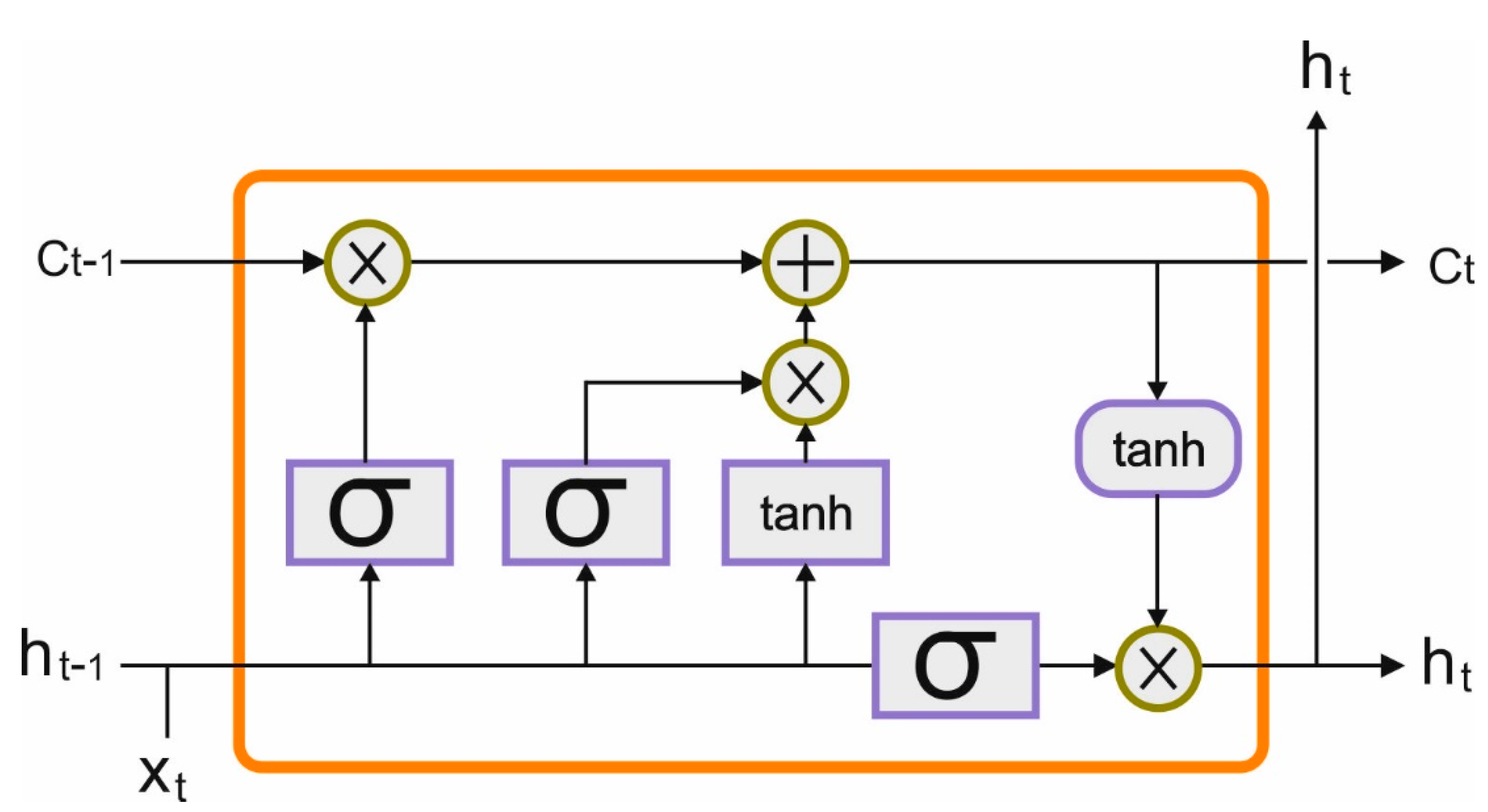
Figure 2 depicts the framework of the LSTM technique.
The structure of the LSTM network node contains 3 fundamental gates, namely the forget gate
, input gate
, and output gate
. However, the input, as well as output gates, signify the data entered and data exit the node at time
correspondingly. The forgetting gate chooses the data to be forgotten related to the preceding status data
and existing input
. These 3 gates choose that upgrade the present memory cell
and present latency
value. During the LSTM node, the connections amongst the gates were computed mathematically utilizing the following formula:
In the LSTM network structure procedures, the representation vectors take as an input in the primary data to the final data. Consider
represent a matrix consisting of a hidden vector
that the LSTM produced, where the size of the hidden layer is represented as
and the length of the given data is denoted by
. Moreover,
represents a vector of ls and
embedding vector. The attention model produces an attention a weighted hidden representation
and weight vector
In the equation, the projection parameters are characterized by and . signifies a weighted representation of data with a given aspect, and a vector consisting of attention weight is indicated as . The attention model enables the model to capture the essential part of data while considering different aspects.
4. Performance Validation
In this study, the performance validation of the EADL-BTMIC model is carried out using the Figshare dataset [
24]. The details related to the dataset are shown in
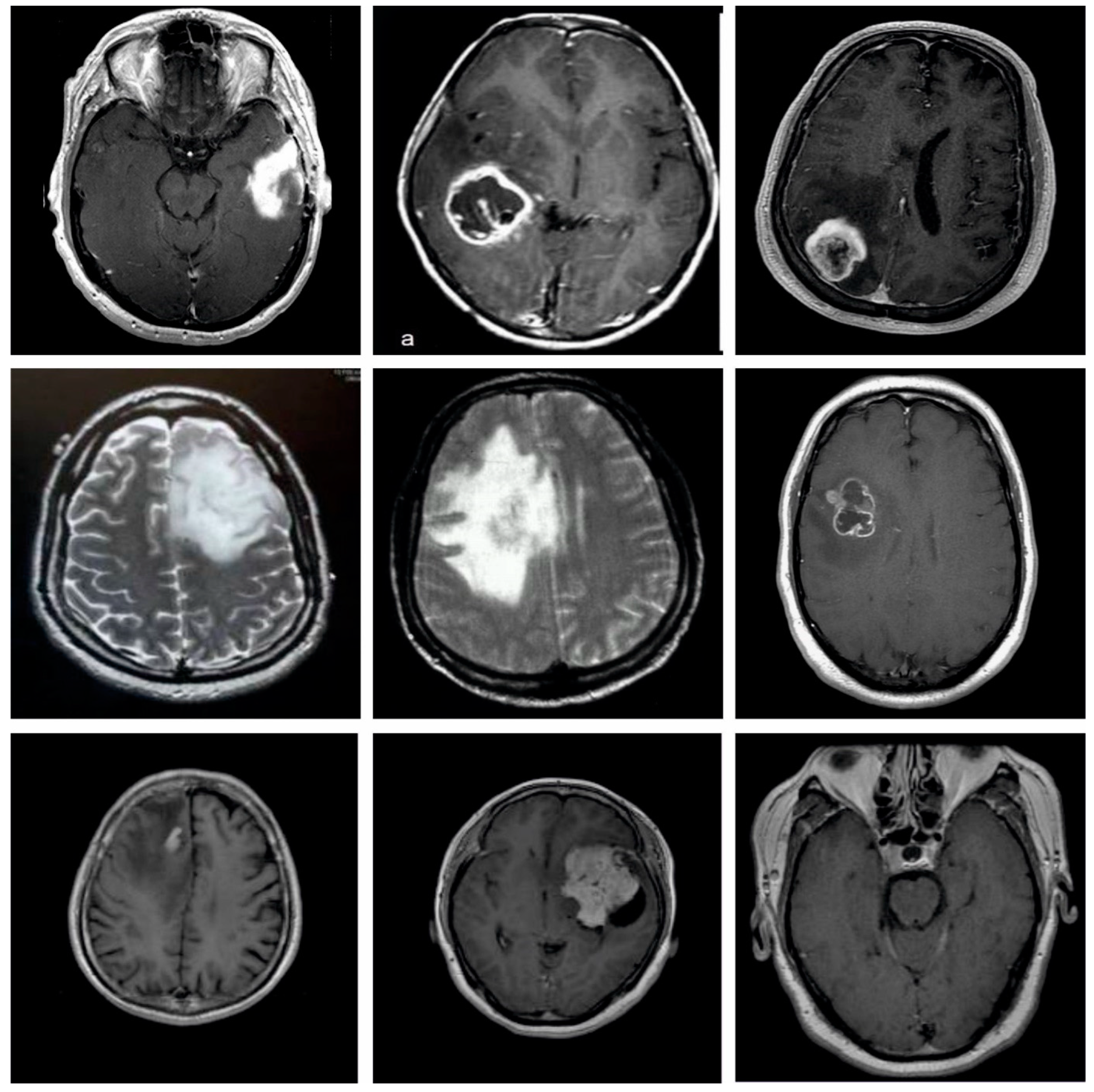
Table 1. A few sample images are illustrated in
Figure 3. The dataset holds 3064 T1-weighted contrast-enhanced images with 3 kinds of BT. The dataset includes 708 images in the Meningioma class, 930 images in the Pituitary class, and 1426 images in the Glioma class. In this study, the experimental validation occurs in two distinct ways by splitting the dataset into two aspects based on the size of the training and testing data: 80% of training with 20% of testing data and 70% of training with 30% of testing data. The proposed model is simulated using Python 3.6.5 tool. The parameter settings are given as follows: learning rate: 0.01, dropout: 0.5, batch size: 5, epoch count: 50, and activation: ReLU.
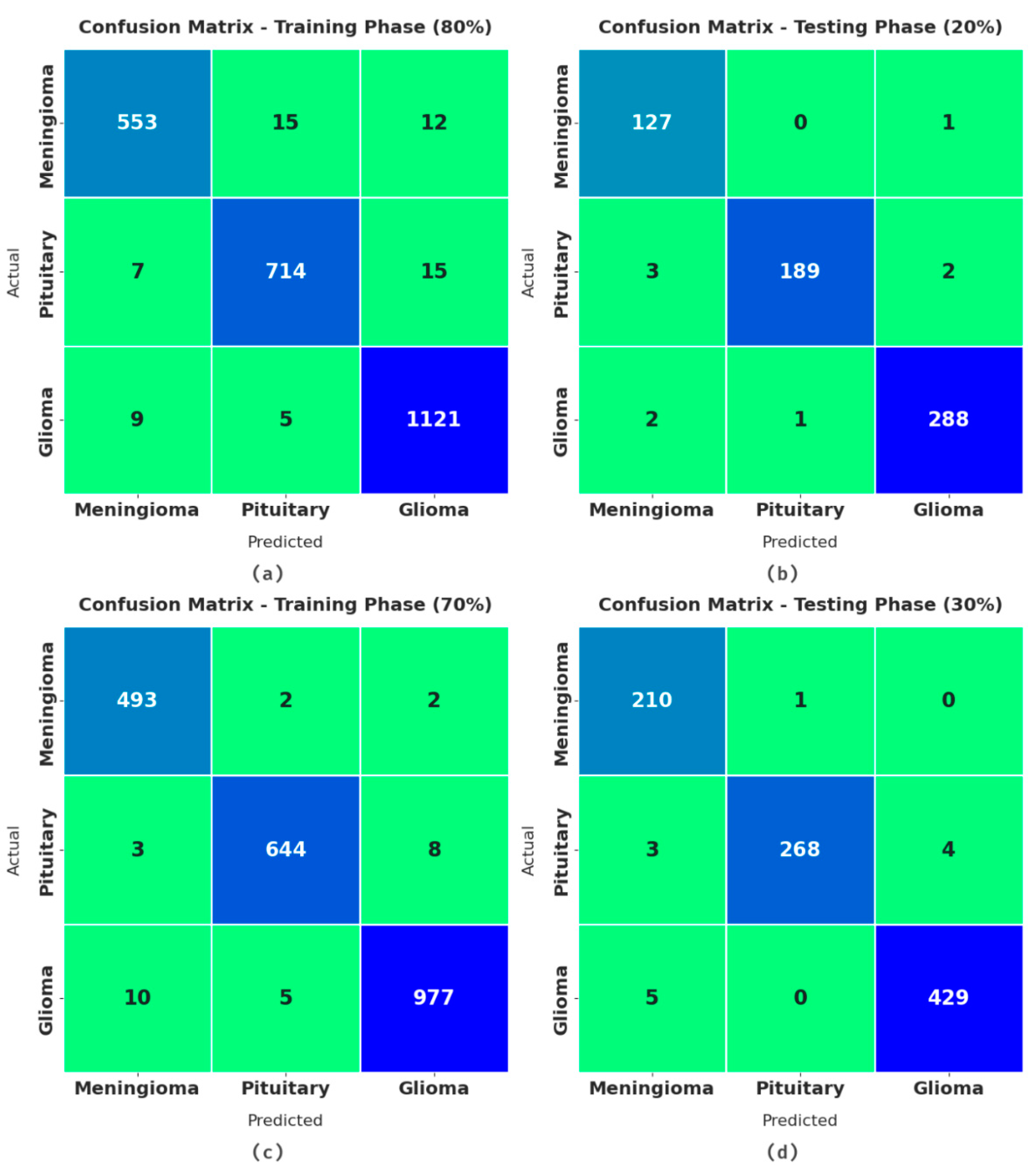
Figure 4 demonstrates the confusion matrices formed by the EADL-BTMIC model on test data. With 80% of TR data, the EADL-BTMIC model identified 553, 7144, and 1121 samples into MEN, PIT, and GLI classes, respectively. In addition, with 20% of TS data, the EADL-BTMIC methodology identified 127, 189, and 288 samples into MEN, PIT, and GLI classes, correspondingly. Additionally, with 70% of TR data, the EADL-BTMIC system identified 493, 644, and 977 samples into MEN, PIT, and GLI classes, correspondingly. Finally, with 30% of TS data, the EADL-BTMIC technique identified 210, 268, and 429 samples into MEN, PIT, and GLI classes, respectively.
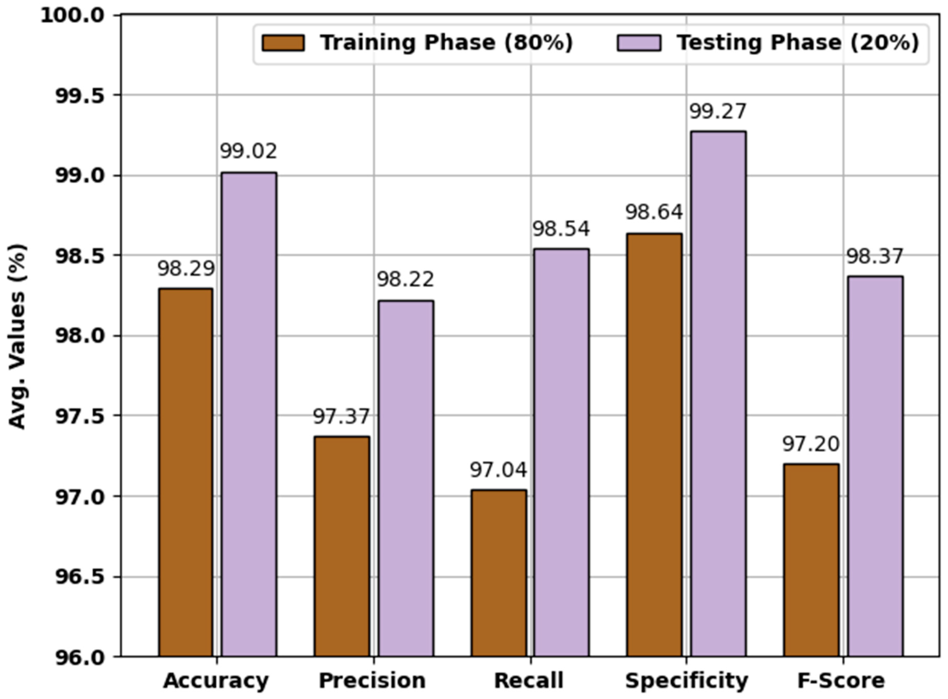
Table 2 and
Figure 5 depict the overall classifier results of the EADL-BTMIC model on 80% of training (TR) data and 20% of testing (TS) data. The experimental values exposed that the EADL-BTMIC technique exhibited effectual outcomes. For instance, with 80% of TR data, the EADL-BTMIC model obtained increased
,
,
,
, and
of 98.29%, 97.37%, 97.04%, 98.64%, and 97.20%, respectively. At the same time, with 20% of TS data, the EADL-BTMIC methodology reached enhanced
,
,
,
, and
of 99.02%, 98.22%, 98.54%, 99.27%, and 98.37%, correspondingly.
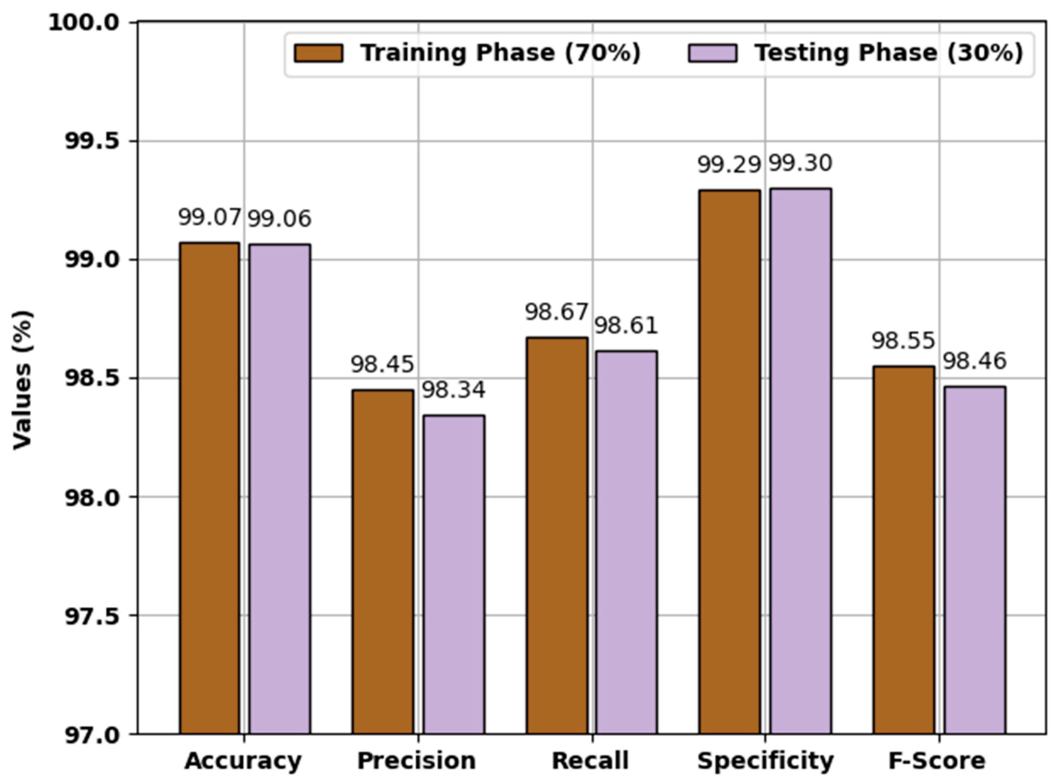
Table 3 and
Figure 6 display the overall classifier results of the EADL-BTMIC technique on 70% of TR data and 30% of TS data. The experimental values revealed that the EADL-BTMIC technique illustrated effectual outcomes.
For sample, with 70% of TR data, the EADL-BTMIC technique attained enhanced , , , , and of 99.07%, 98.45%, 98.67%, 99.29%, and 98.55%, correspondingly. Simultaneously, with 30% of TS data, the EADL-BTMIC approach reached increased , , , , and of 99.06%, 98.34%, 98.61%, 99.30%, and 98.46%, correspondingly.
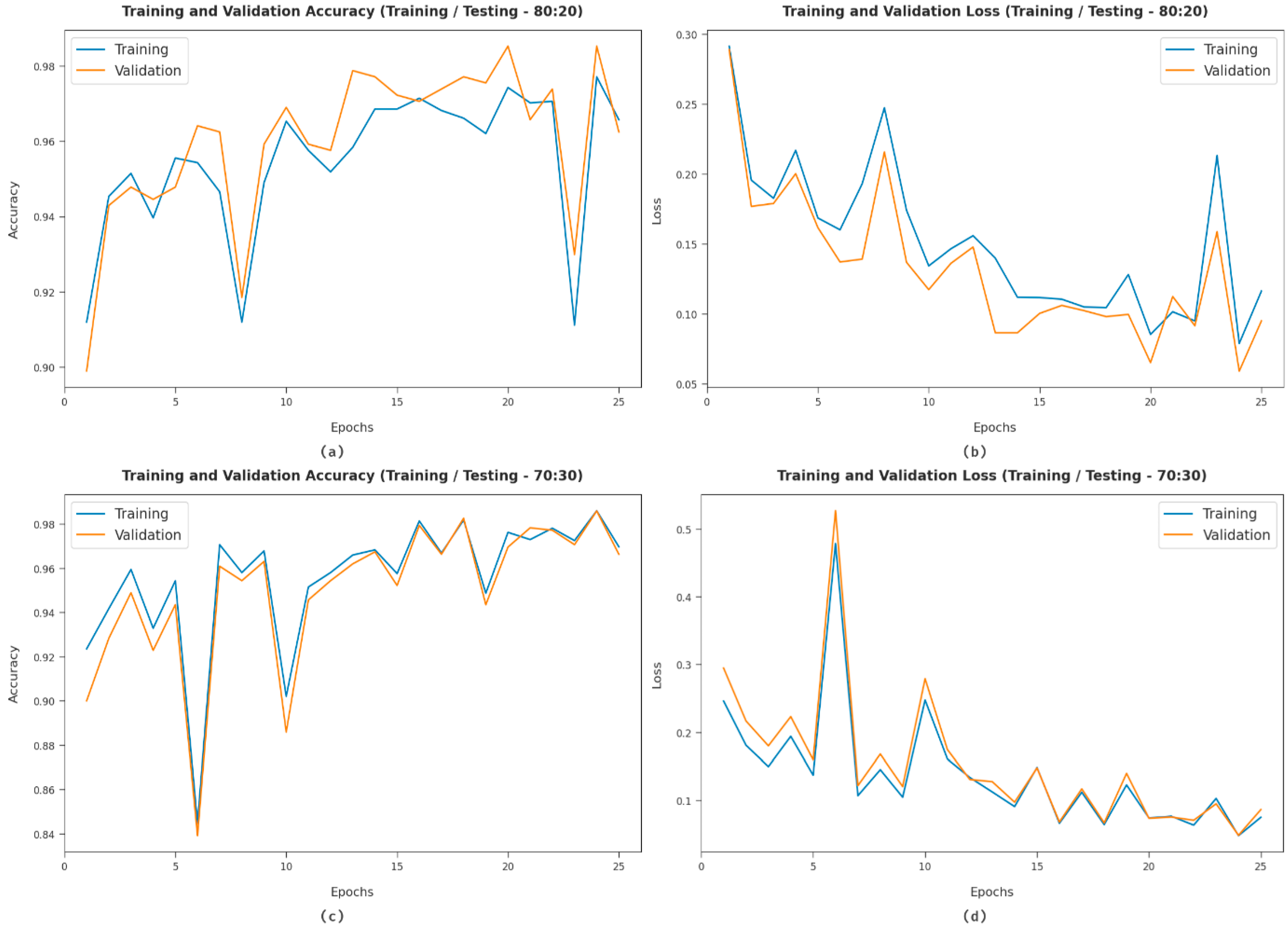
Figure 7 offers the accuracy and loss graph analysis of the EADL-BTMIC approach on a distinct set of TR/TS datasets. The outcomes demonstrated that the accuracy value is enhanced, and the loss value tends to reduce with a higher epoch count. It is also observed that the training loss is minimal, and validation accuracy is superior on distinct sets of TR/TS datasets.
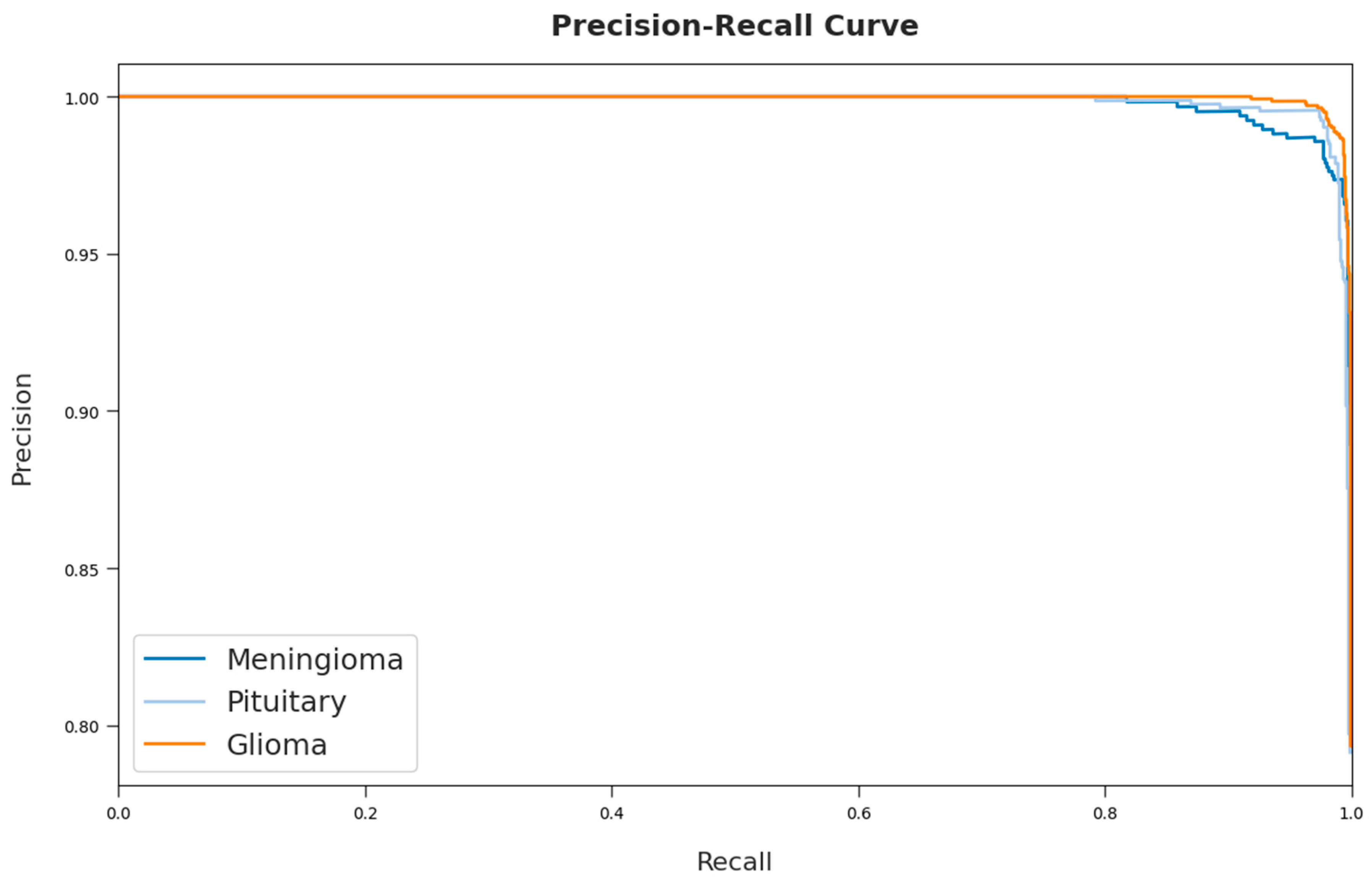
A brief precision-recall examination of the EADL-BTMIC model on the test dataset is portrayed in
Figure 8. By observing the figure, it is noticed that the EADL-BTMIC model has accomplished maximum precision-recall performance under all classes.
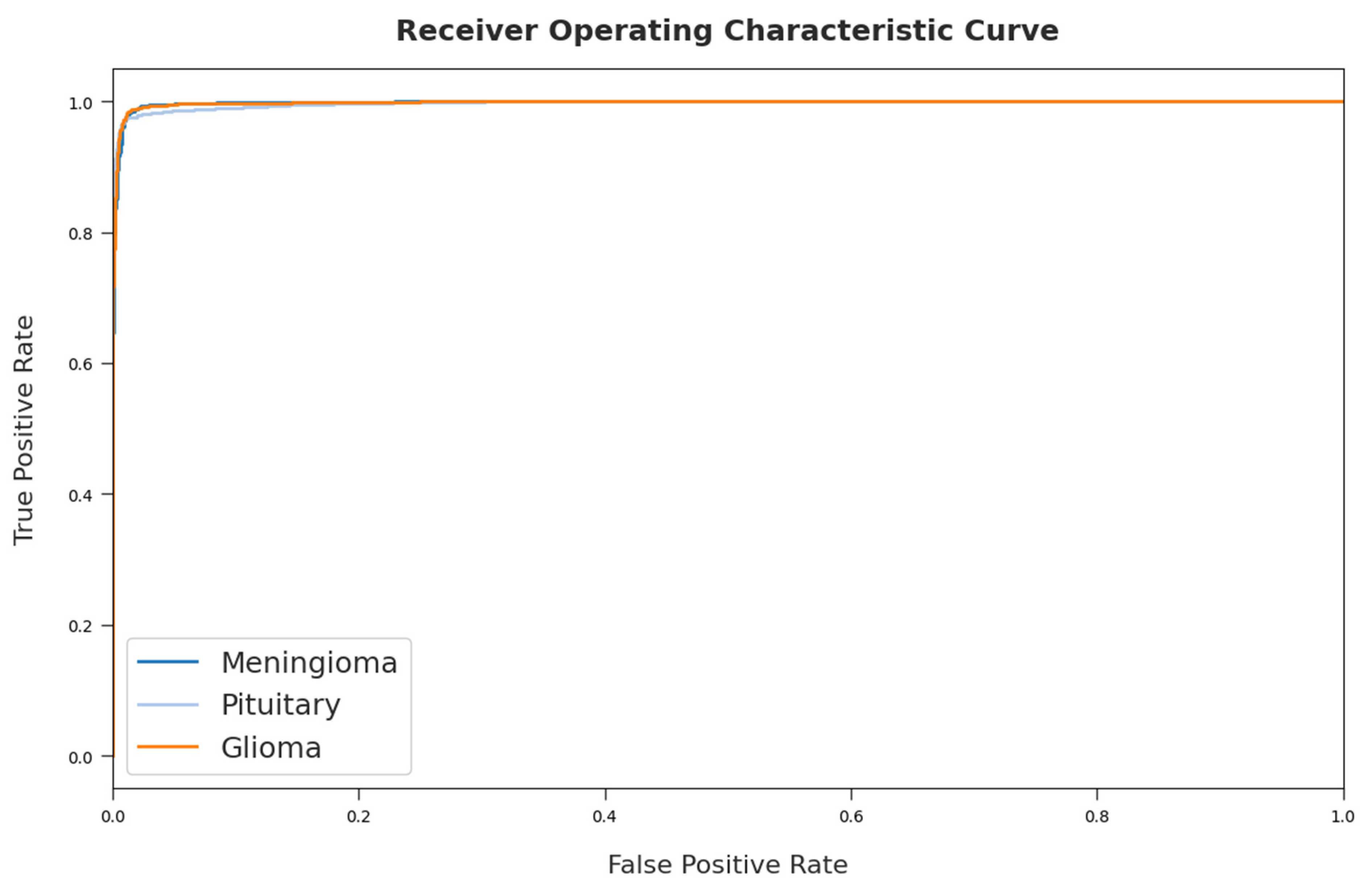
A detailed ROC investigation of the EADL-BTMIC model on the test dataset is portrayed in
Figure 9. The results indicated that the EADL-BTMIC model exhibited its ability to categorize three different classes, such as meningioma, pituitary, and glioma, on the test dataset.
Table 4 provides a comprehensive comparison study of the EADL-BTMIC model with other models [
15,
17].
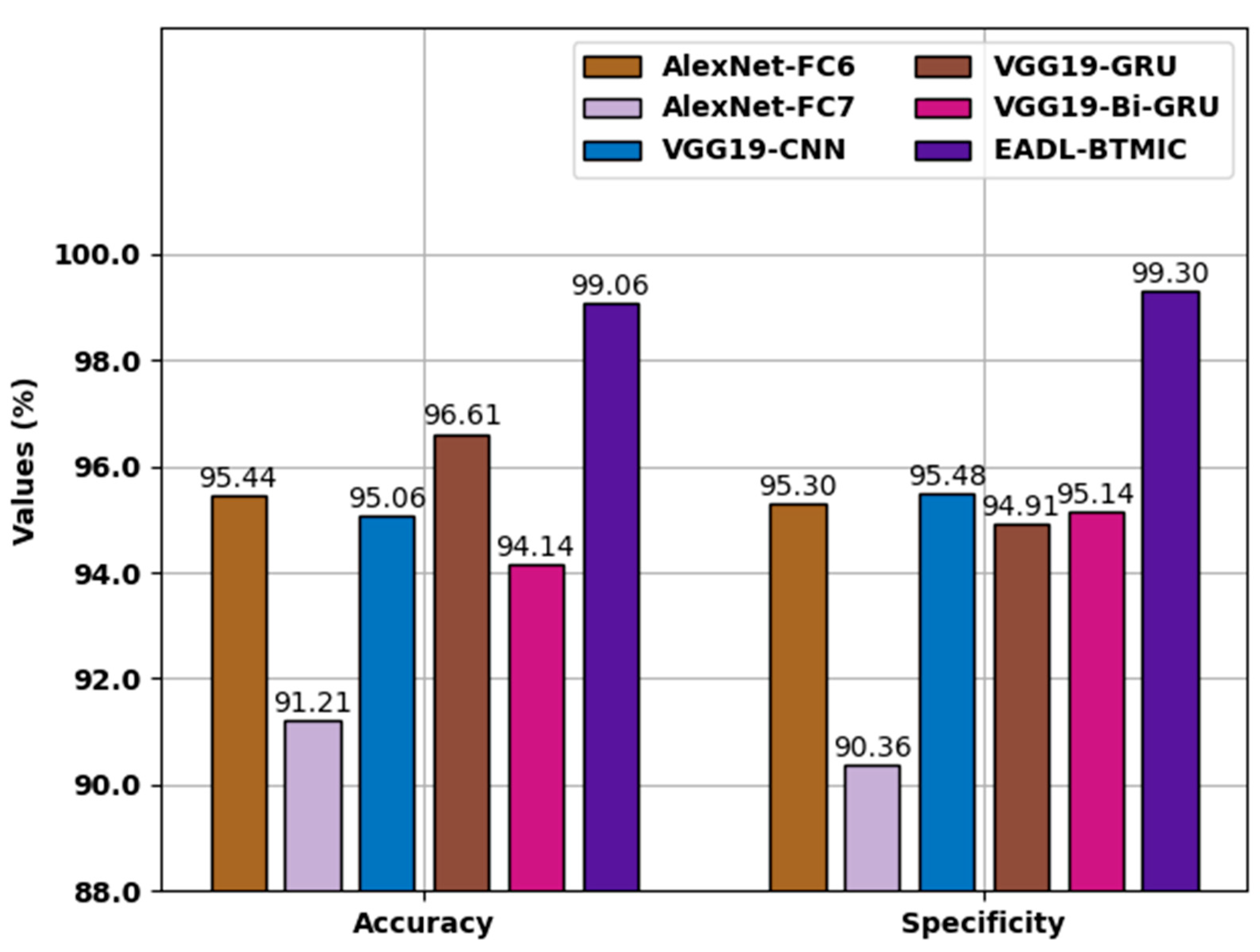
Figure 10 demonstrates a brief
and
assessment of the EADL-BTMIC approach with existing models. The figure indicates that the AlexNet-FC7 method has shown lower performance with minimal
and
of 91.21% and 90.36%, respectively. Followed by the Alexnet-FC6, VGG19-CNN, VGG19-GRU, and VGG19-Bi-GRU models, which accomplished moderately closer values of
and
. However, the EADL-BTMIC model has gained maximum
and
of 99.06% and 99.30%, respectively.
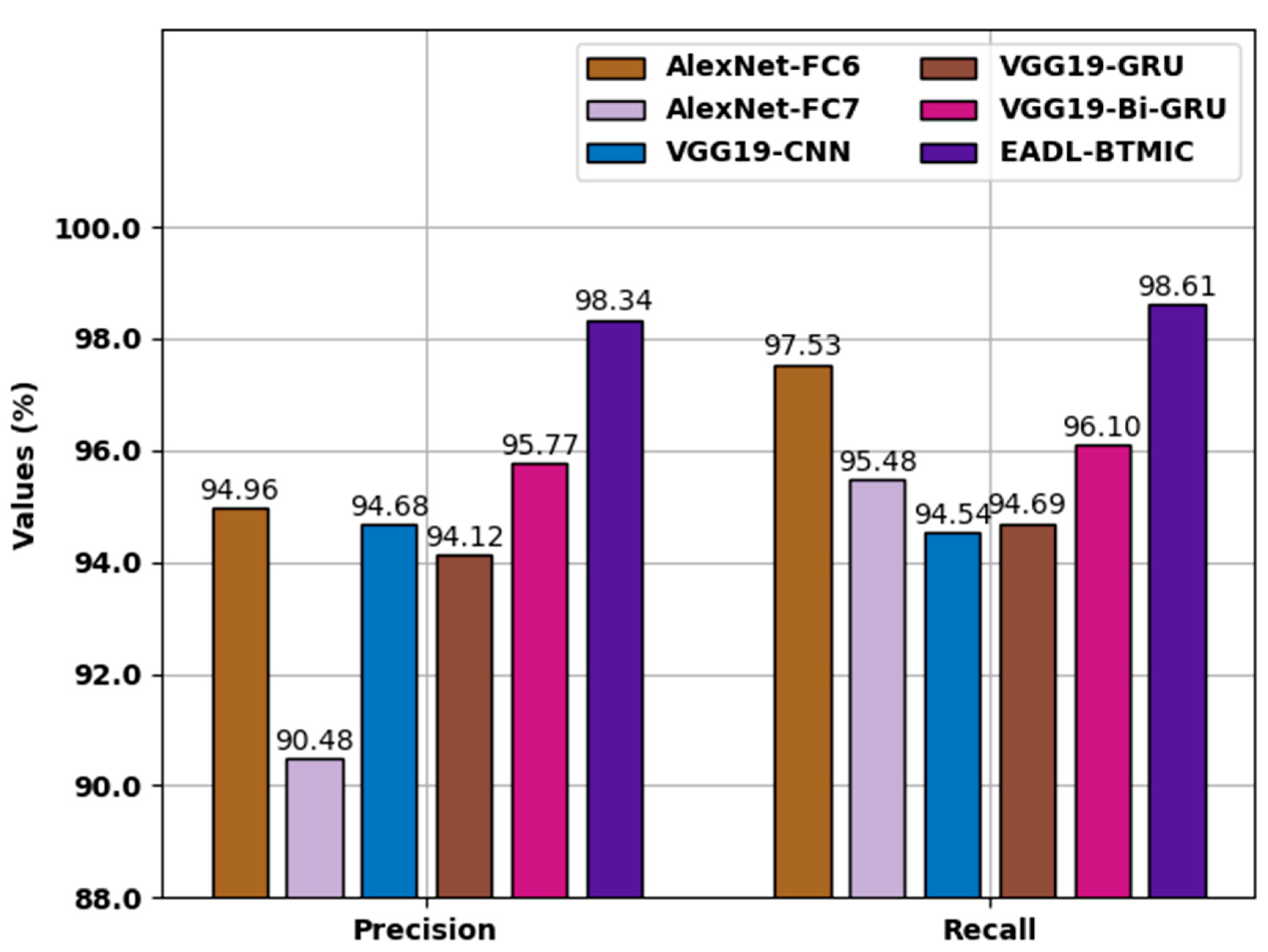
Figure 11 illustrates a detailed
and
analysis of the EADL-BTMIC system with recent methods. The figure shows that the AlexNet-FC7 algorithm has shown lower performance with minimal
and
of 90.48% and 95.48%, correspondingly. Afterward, the Alexnet-FC6, VGG19-CNN, VGG19-GRU, and VGG19-Bi-GRU techniques accomplished moderately closer values of
and
. Finally, the EADL-BTMIC technique gained maximal
and
of 98.34% and 98.61%, correspondingly.
The above-mentioned results and discussion ensured that the EADL-BTMIC model resulted in enhanced classification outcomes over other methods.


 ,
, 


