DETECT-LC: A 3D Deep Learning and Textural Radiomics Computational Model for Lung Cancer Staging and Tumor Phenotyping Based on Computed Tomography Volumes

Abstract

Lung Cancer is one of the primary causes of cancer-related deaths worldwide. Timely diagnosis and precise staging are pivotal for treatment planning, and thus can lead to increased survival rates. The application of advanced machine learning techniques helps in effective diagnosis and staging. In this study, a multistage neurobased computational model is proposed, DETECT-LC learning. $DETECT$-$LC$ handles the challenge of choosing discriminative CT slices for constructing 3D volumes, using Haralick, histogram-based radiomics, and unsupervised clustering. ALT-CNN-DENSE Net architecture is introduced as part of $DETECT$-$LC$ for voxel-based classification. $DETECT$-$LC$ offers an automatic threshold-based segmentation approach instead of the manual procedure, to help mitigate this burden for radiologists and clinicians. Also, $DETECT$-$LC$ presents a slice selection approach and a newly proposed relatively light weight 3D CNN architecture to improve existing studies performance. The proposed pipeline is employed for tumor phenotyping and staging. $DETECT$-$LC$ performance is assessed through a range of experiments, in which $DETECT$-$LC$ attains outstanding performance surpassing its counterparts in terms of accuracy, sensitivity, F1-score and Area under Curve (AuC). For histopathology classification, $DETECT$-$LC$ average performance achieved an improvement of 20% in overall accuracy, 0.19 in sensitivity, 0.16 in F1-Score and 0.16 in AuC over the state of the art. A similar enhancement is reached for staging, where higher overall accuracy, sensitivity and F1-score are attained with differences of 8%, 0.08 and 0.14.

1. Introduction

Cancer is considered one of the principal causes of death, impeding the possibility of increasing life expectancy worldwide. According to GLOBOCAN estimates of cancer incidence and mortality in 2020, lung cancer is responsible for around 18% of cancer-related deaths. Newly diagnosed lung cancer cases are estimated to be 2.2 million cases. Lung cancer ranks first in men and third in women in terms of incidence [1]. According to North American Association of Central Cancer Registries (NAACCR), it was projected that 235,760 lung cancer cases out of 1,898,160 new cancer cases will be attributed to lung cancer in the United states of America (USA) [2] in 2021. It is also projected that lung cancer will account for 131,880 out of 608,570 new deaths will be attributed to in the USA [2] in 2021. Meanwhile, lung cancer mortality manifests an accelerating long-term decline, which doubled from 2.4% during 2009 through 2013 to 5% during 2014 through 2018 for both sexes [2]. Non-small cell lung cancer (NSCLC), specifically, has attained a significant gain of 5 to 6% in survival for every stage of diagnosis. Non-small cell lung cancer (NSCLC) represents 80 to 85% of lung cancers [2].

Several factors have been found to contribute to the reported survival gains in the USA. These factors include rising medical care access by individuals due to the Patient Protection and Affordable Care Act and Medicaid expansion in 2014 [3]. More importantly, the developments in diagnostics and lung cancer staging [4] fields have led to increased survival in early stage cancers. Lung cancer staging is crucial for therapy planning and thus has a significant positive prognostic effect [4]. Medical imaging is one of the fundamental steps for effective staging. Different modalities are available for lung imaging and screening, such as Magnetic Resonance Imaging (MRI), Computed Tomography (CT) and Positron Emission Tomography (PET) scans. However, CT remains the standard imaging modality for preoperative staging. CT imaging has the advantages of lower cost and shorter examination time, together with its comparable performance [5] relative to other imaging modalities.

Recently, machine learning (ML) and deep learning (DL) have shown epic potential in enhancing clinical decision making [6]. In oncology, ML and DL are applied in the diagnosis and staging phase, as well as the follow-up and treatment evaluation phase [7]. The immense advances in ML techniques and the availability of computationally powerful devices enable the effective processing of volumetric imaging data for diagnostic and staging purposes [8].Volumetric data, for CT scans, is composed of two dimensional (2D) stacked images, that gives better representation of the lung. Such enhanced representation is generally related to improved performance [9]. However, the election of meaningful 2D slices for 3D volume reconstruction, has a considerable impact on the performance. In this paper, DETECT-LC pipeline is proposed for Non-small cell lung cancer (NSCLC) diagnosis and staging. The pipeline incorporates:

• A simple automatic segmentation technique using hounsfield unit values and subsequent thresholding with acceptable performance.
• A semi-supervised 2D slice election approach, which depends on textural features. The adopted clustering-based approach eliminates the need for extensive human intervention, allowing for faster processing.
• A simple 3D DL network architecture ALT-CNN-DENSE Net for effective lung cancer staging and tumor phenotyping. The performance of the proposed network surpasses the performance of the state of the art.

This paper is organised as follows: a brief background on lung cancer staging standard will be given in the next section. Similar studies that performed staging and/or malignancy detection will be presented in Section 3. In Section 4, the proposed staging pipeline will be described DETECT-LC. The benchmark datasets used to test the performance of DETECT-LC are depicted in Section 5, with our obtained results and subsequent discussion. Conclusions are finally drawn in Section 6.

2. Background

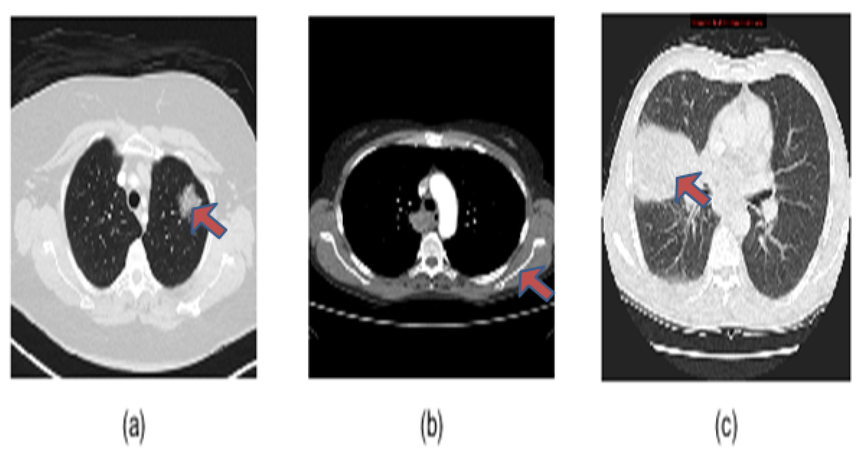
In this study, we will focus on NSCLC diagnosis and staging. NSCLC includes three main subtypes namely adenocarcinoma, squamous cell carcinoma, and large cell carcinoma. Despite the subtypes differences regarding their onset cell sites, they are grouped together due to their similarity in terms of treatment and prognosis. Figure 1 illustrates the manifestations of the three NSCLC subtypes on CT scans. The characteristics of these subtypes on CT scans [10] can be summarized as follows:

• Adenocarcinoma (ADC) early manifestation is in mucous cells and shows as rounded or irregular lung nodules of higher attenuation. These nodules are usually present at the outer parts of the lung.
• Squamous Cell Carcinoma (SCC) appears first in squamous cells at the inside lining of the lung airways. These tumors are often white in color. Typically, SCC spread centrally in the hilar cavity but can extend peripherally to the chest walls, as indicated in Figure 1.
• Large cell (undifferentiated) carcinoma (LCC) has the tendency to grow rapidly anywhere in the lung, which makes its survival rate low. Additionally, it lacks the presence of distinctive features except for large nuclei with modest amount of cytoplasm microscopically.

Figure 1. NSCLC radiopathological subtypes manifestations (marked) on CT scans: (a) Adenocarcinoma (b) Squamous Cell Carcinoma (c) Large Cell (undifferentiated) Carcinoma.

Figure 1. NSCLC radiopathological subtypes manifestations (marked) on CT scans: (a) Adenocarcinoma (b) Squamous Cell Carcinoma (c) Large Cell (undifferentiated) Carcinoma.

Within each carcinoma subtype, staging is crucial for effective treatment and follow up planning. The International Association for the Study of Lung Cancer (IASLC) recommends a standard procedure for cancer stage classification based on TNM staging [11]. The assigned cancer category relies on three aspects: the size of the primary tumor (T), the number and location of regional lymph nodes (N), and the presence or absence of metastasis (M). The proposed classification system aims to provide a uniform system for consistent reproducible stage, which is necessary for optimizing treatment. According to the 8th Edition TNM staging update [11], there are 13 stages depending on different combinations of T, N and M variations. In this study, we will focus on four broad stage categorizations, namely stage I, stage II, stage IIIA and stage IIIB. Detailed definition of the stages can be found in the 8th Edition TNM staging update [11]. These stages represent localised and regional cancer spread with higher expected survival rates [12]. Hence, timely accurate staging is of immense importance to help optimize the therapeutic outcome.

3. Related Work

Oncology computer aided diagnostic tools have evidently evolved over the years. ML-based tissue and tumor segmentation models have been widely proposed as auxiliary diagnostic tools. Two examples of the recent work on segmentation are Nazir et al. [13] and Nishio et al. [14]. In Nazir et al. [13] approach, adaptive global threshold is applied for lung segmentation. The threshold is elected based on CT image histogram. Following segmentation, laplacian pyramids are used for image decomposition and reconstruction. Adaptive Sparse representation is used for image fusion. Nishio et al. [14] used transfer learning pretrained on an artificial dataset LUNA16. The artificial dataset was generated with the aid of Generative Adversial Network and 3D graph cut. The pretrained segmentation model is constructed by nnUnet, where it showed 0.09 higher dice similarity score than without transfer learning.

Despite that lung segmentation is an important step for subsequent diagnosis, tools that perform solely segmentation fail to utilize the full capability of ML. Hence, various studies were directed towards providing a complete solution for pathology diagnosis and/or stage assessment. To this end, Chaunzwa et al. [15] compared the performance of fully connected VGG16 Convolution Neural Network (CNN) classification to traditional ML classifiers. The classification models were used to differentiate between ADC and SCC. The traditional classifiers relied on 512 and 4096 feature vectors output from VGG16 architecture. The highest performance was achieved through a deep-radiomics approach, where a 4096 feature vector is obtained from the last fully connected layer. Principal component analysis and Least Absolute Shrinkage and Selection Operator (LASSO) method were used to generate and select the most relevant features. Then, k-Nearest Neighbors (kNN) (k = 5) is applied for classification. Marentakis et al. [16] conducted an extensive comparison between various approaches: two classifiers radiomics (kNN and SVM), four recent CNN architectures, CNN with Long Short Term Memory (LSTM) and combinatorial approach (CNN + LSTM + radiomics). LSTM was used to incorporate spatial coherence of CT slices into the model. LSTM + Inception attained the highest accuracy and AuC. Another study based on radiomics is the work of Khodbashki et al. [17]. A set of 1433 radiomics features were generated from wavelet decomposition and LOG filtered images. Wrapper and Multivariate regression feature selection algorithms were applied to classify histopathological subtypes. Traditional learning was also adopted by Yang et al. [18]. A total of 788 radiomic features were extracted then various features selection methods were used to select the most informative features. Logistics Regression (LR), Support Vector Machines (SVM), and Random Forest (RF) were applied for histology (SCC and ADC) determination.

Other studies were directed towards staging, such as the work of Yu et al. [19]. Image segmentation and features extraction are done using 3D-Slicer software and Pyradiomics package respectively. SMOTE oversampling was applied to balance the dataset. Random Forest was used for staging. The model did not perform well on multi-class staging, hence binary (early-late) staging was performed resulting in accuracy of 75%. Choi et al. [20] also performed binary staging with a serial two phase system. U-net autoencoder network is used for latent variables extraction and image reconstruction. Then, CNN architecture is used for binary classification. U-net + CNN outperformed U-net + traditional machine learning classifiers. Paing et al. [21] performed T-staging using Back Propagation Neural Network (BPNN). Five classifiers were applied on merged benchmark datasets. BPNN achieved the highest accuracy of 90.6% with 28 geometric, intensity and textural nodule features. Another study that implemented cascaded deep networks is that of Moitra et al. [22]. Maximally stable extremal regions (MSER) and speeded up robust features (SURF) were extracted from enhanced images. The extracted features are fed to a 1D CNN-RNN model for multi-staging. The model achieved the highest accuracy compared to RF, SVM and Multilayer Perceptron.

Some of the previous work relied on manual intervention and/or expert knowledge for Region of Interest (RoI) specification such as the work of Choi et al. [20]. Human intervention provides validation for this step. However, fully automating the processing pipeline would mitigate the burden off clinicians and radiologists. Hence, automating the step of RoI specification is needed. The expected benefit is to enhance the performance of diagnostic systems and free clinicians and radiologists to handle more critical tasks. Also, most of the presented studies were directed towards histology classification or binary staging [15,16,19,20], whereas multiclass staging can be considered more crucial. Multiclass staging is important for adapting the medical care provision plans and providing better prognosis. Also, the stratification of survival rates varies considerably with the respective stage [12]. Thus, studies are needed to address this higher complexity classification problem of multistaging to be able to provide precise treatment plans. Additionally, some of the available studies did not utilize the spatial coherence information available in 3D CT volumes [21] missing the holistic context of the slices. Neglecting the connectivity properties of CT image pixels may disadvantage the staging decision. Another limitation in 2D slice-based classification, which offers a slice by slice class, is that it does not produce a patient-level decision. Such limitation restricts these studies diagnostic value, as it does not provide an overall diagnosis per patient. Thus, 3D volumetric decision support systems are called for to produce patient decision. On the other hand, studies that used 3D volumes utilized computationally expensive architectures [15,22]. Another issue with processing 3D volumes is selecting informative slices from the CT series. Slice selection is critical to construct informative 3D volumes. Selection eliminates the effect of irrelevant slices on performance and reduces computational time. However, this issue was not inspected, to our knowledge, in the literature [15,20,22]. Despite the existing shortcomings, the employment of ML and deep learning in lung cancer decision support systems show substantial prospect in various applications [23]. Such potential encourages further developments that consider the issues and limitations in current studies in attempt to improve the tumor phenotyping and staging performance. Therefore, this study aims to tackle the existing described issues through our proposed framework. It provides an automatic threshold-based segmentation approach, a semisupervised slice selection approach and a newly proposed relatively lightweight 3D CNN architecture.

4. Materials and Methods

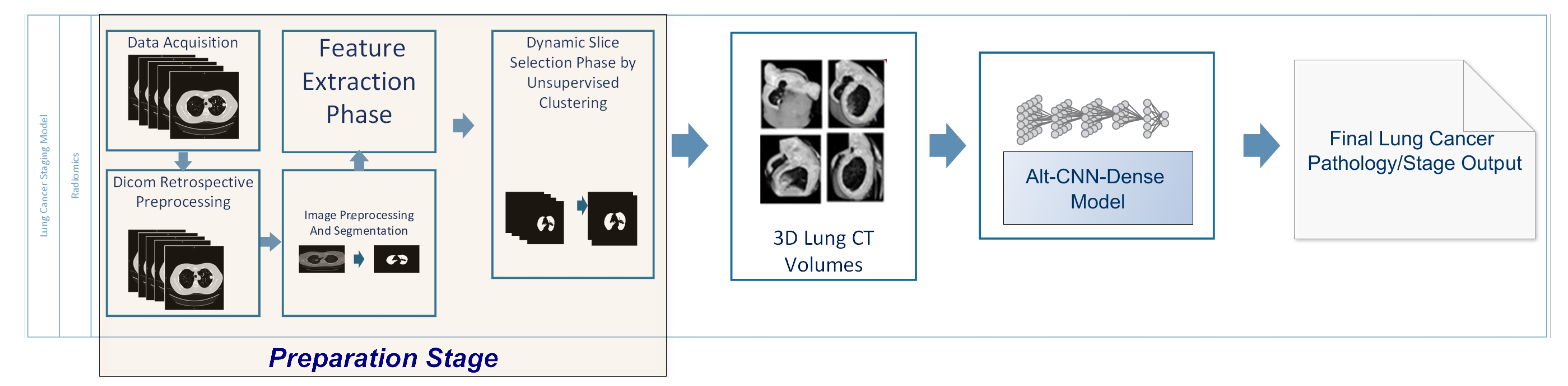
In this study, a 3D volumetric multi-stage computational pipeline is proposed (shown in Figure 2) for Lung Cancer pathology phenotyping and staging integrating 3D DEep Learning and TExtural Radiomics applied on CT volumes (DETECT-LC). The pipeline is used for producing carcinoma subtype or stage class.

In order to reduce the computation power required for processing 3D volumes and enhance the effectiveness of the proposed CNN model, a semi-supervised slice selection procedure is suggested. The selection procedure assists in constructing informative and concise 3D volumes. The created 3D volumes are input to the new ALT-CNN-DENSE Model architecture. The model outputs the corresponding class. Figure 2 depicts the flow of the decision process through the different computational pipeline phases. A detailed description of each phase is provided.

4.1. Dataset Acquisition

Three publicly available benchmark datasets from TCIA Repository [24] are used to train, validate and test $DETECT$-$LC$. The datasets are NSCLC Radiomics [25], NSCLC Radio-Genomics, NSCLC Radiomics-Genomics [26]. Several studies have been experimented with these datasets, which allows state of the art comparison with our model. In addition, it includes thoracic cavity binary segmentation masks, which enables the validation of our simple segmentation approach.

NSCLC Radiomics (Lung 1) includes 422 non-small cell lung cancer (NSCLC) patients’ pre-treatment CT scans. After the applied preprocessing, the dataset is set to be 395 volumes. On average, there are 123 slice/patient. Clinical data is provided together with the CT scans.

NSCLC Radiomics-Genomics (Lung 3) holds pre-treatment CT scans, gene expression, and clinical data of 89 non-small cell lung cancer (NSCLC) patients. The included patients were treated with surgery.

NSCLC Radio-Genomics is a cohort of 211 patients, where imaging data are also paired with gene mutation, RNA sequencing data from samples of surgically excised tumor tissue. Also, clinical data including survival outcomes are provided.

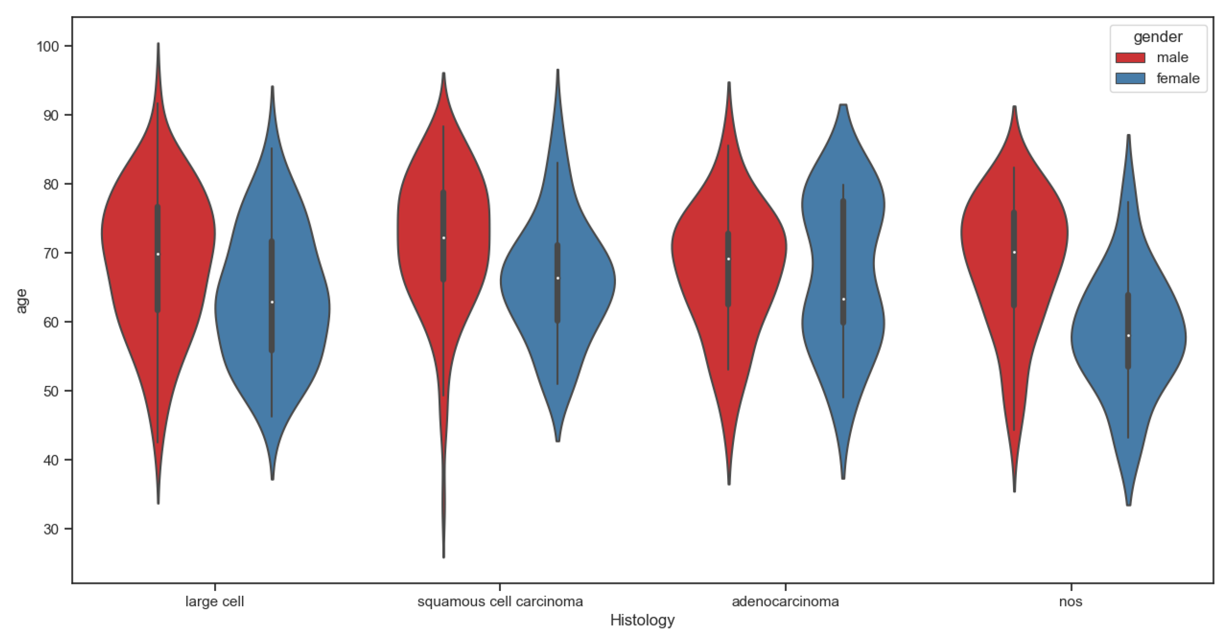
For each dataset, the distribution of patients across the various histology groups and stages is shown in

Table 1. Stage and Pathology (ADC, SCC, NOS and LCC) Distribution in the Non-Small Cell Lung Cancer Benchmark Datasets.

NSCLC Radiomics (Lung 1)
	ADC	SCC	NOS	LCC
I	11	23	44	15
II	8	23	4	5
IIIA	14	44	15	36
IIIB	18	62	NA	57
NSCLC Radiomics-Genomics
	ADC	SCC	NOS
I	5	9	25
II	23	23	9
IIIA	3	4	NA
IIIB	5	6	NA
NSCLC Radio-Genomics
	ADC	SCC	NOS
I	73	18	2
II	22	12	NA
IIIA	15	5	1
IIIB	2	NA	1
UD	60	NA	NA

UD: Unspecified.

. In addition, the age distribution of subjects across stages I, II, IIIA and IIIB (gender differentiated) is illustrated in Figure 3. The violin plot shows no significant difference in terms of age between different stage groups (p = 0.067, Mann-Whitney U test).

The datasets included carcinoma subtypes and stages that are out of the scope of the specified classes. Hence, their respective records were eliminated. The typical data used in our experiments are outlined in Table 1.

4.2. Data Preprocessing

DICOM retrospective preprocessing is applied on CT slices in order to convert slice domain from imaging machine domain to CT Hounsfield Unit (HU) domain. Domain transformation relies on the differences in the absorption/attenuation coefficients of radiation (X-ray beam) within tissues. The HU value of a tissue can be computed based on the linear attenuation of the tissue ($\mu$) relative to the attenuation of water (${\mu }_{water}$) and air (${\mu }_{air}$) under standard temperature and pressure as expressed in Equation (1).

$$HU=1000\times \frac{\mu -{\mu }_{water}}{{\mu }_{water}-{\mu }_{air}}$$

(1)

The radiodensity of water is considered to be zero HU and air is −1000 HU. In order to generate grayscale images during CT reconstruction, the intensity values are transformed to HU CT values. Equation (2) is used for transformation, where m is the rescale slope and c is the rescale intercept. The rescale values are available as part of each CT slice metadata.

$$HU=mx+c$$

(2)

Following HU conversion, a binary image (mask) is generated for each slice depending on HU values. Multilevel thresholding is applied based on established HU spectral bands [27], where the lung HU values range from −900 to −400. The mask helps highlight the lung tissue area for further processing. In addition, Gaussian filter is applied on the original slices to remove the noise. The noise might have been generated from electromagnetic waves and heat or light from surroundings.

4.3. Radiomics-Based Semi-Supervised Slice Selection

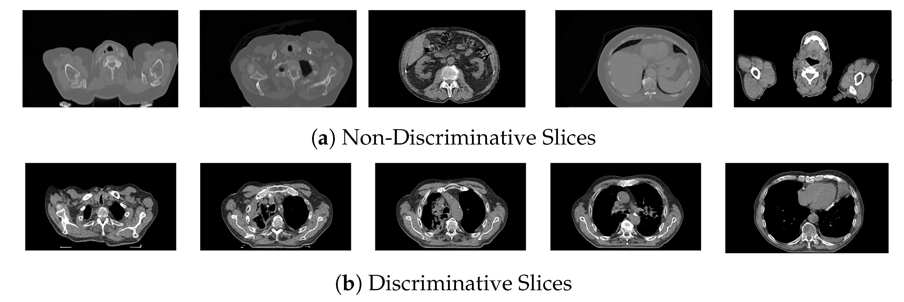
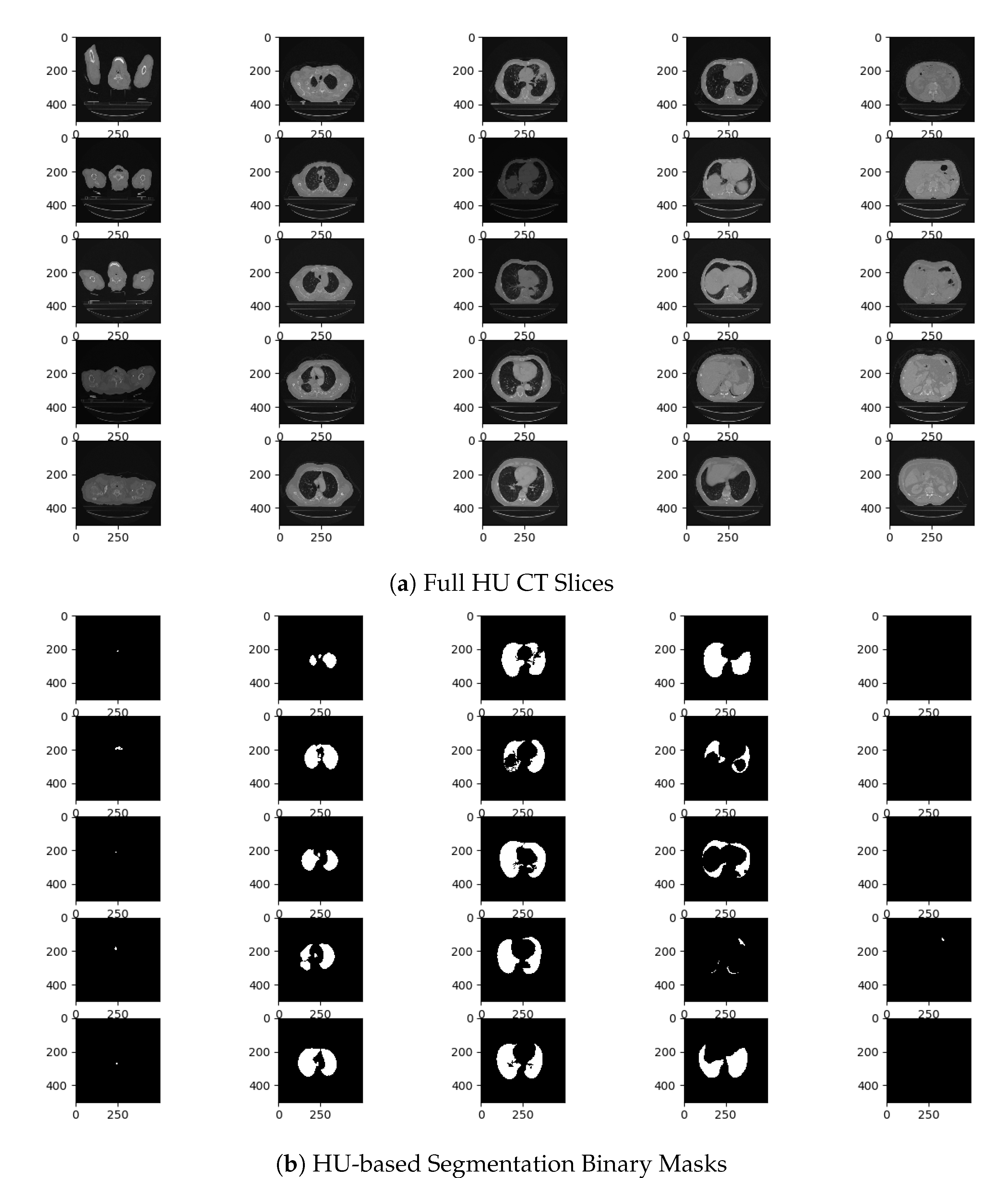
CT scan volumes can be of large number of slices, which leads to high computation time and complexity. Aside from the high computation complexity, another critical issue is the information content of the slices. CT volumes comprise slices of the whole thoracic cavity area. It includes discriminative and non-discriminative lung slices. Figure 4 shows sample slices, exemplar slices in Figure 4a is of low value to the current study as it will not give any additional information to the learning model. In fact, these slices may add noise degrading the performance of the classification model. On the contrary, the exemplar slices in Figure 4b are the ones that need to be selected as they show lung tissue clearly. Another issue is that the exact location (index) of informative slices varies individually per patient, which means that manual selection would be time consuming. Also, static predefined range for the targeted slices will hinder the learning process as the range of informative slices varies considerably. Hence, the slice selection is required to input informative slices to the classifications’ models. The slices are not labelled as discriminative and non-discriminative lung slices; hence, unsupervised clustering is used to group the slices based on a set of extracted features. Unsupervised learning provides an adequate solution to the issue of unlabeled slices, as it divides the slices into their natural groupings based on the extracted features.

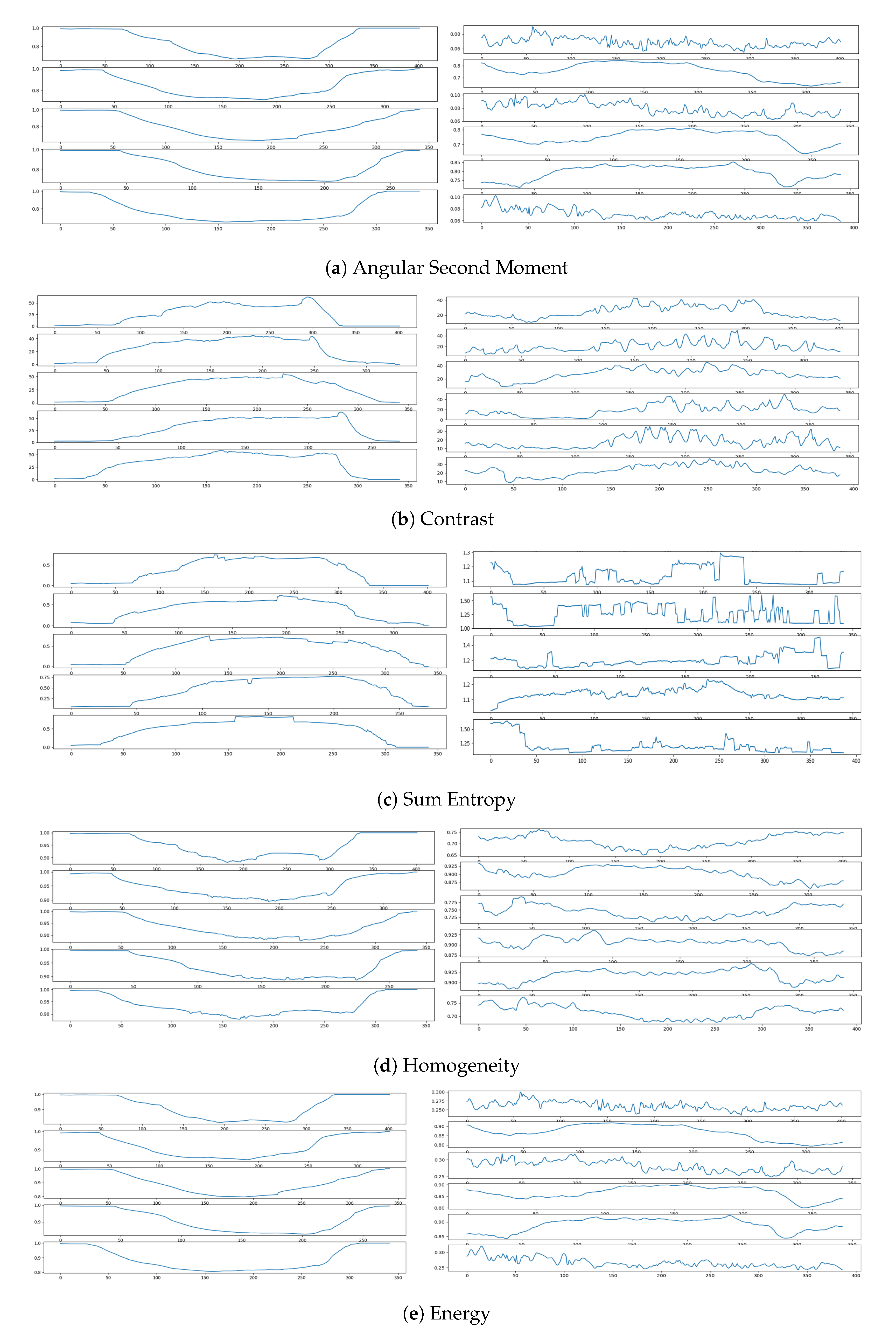
For the purpose of feature extraction, Haralick texture features [28] and Histrogram-based features [29] are extracted from each slice and its binary mask. The features capture the structural and spatial characteristics of the slices. The extracted features help differentiate between discriminative and non-discriminativelung slices. Haralick features are extracted from the normalized Gray-Level Co-occurrence Matrix (GLCM). Each GLCM element $p(i,i)$ represents the co-occurrence of a pair of grey levels $(i,j,d,\theta )$ in neighboring pixels, where i denotes the grey level in the reference pixel, j denotes the grey level in the neighbor pixel, d is the interpixel distance set to one and $\theta$ is the angle of offset between neighbouring pixels set to zero. The number of (quantized) grey levels is denoted as G. Five features are extracted from the produced GLCM, namely Angular Second Moment ($ASM$), contrast (C), Sum Entropy ($SE$), Homogeneity (H) and Energy (E). The equations given below present the calculation of the Haralick features.

$$\begin{array}{cc}& ASM={\sum }_{i=1}^G{\sum }_{j=1}^{G}p{(i,j)}^2\end{array}$$

(3)

$$\begin{array}{cc}& C={\sum }_{i=1}^G{\sum }_{j=1}^G{(i-j)}^{2}p{(i,j)}^2\end{array}$$

(4)

$$\begin{array}{cc}& SE=-{\sum }_{i=1}^G{\sum }_{j=1}^{G}p(i,j){log}_{2}p(i,j)\end{array}$$

(5)

$$\begin{array}{cc}& H={\sum }_{i=1}^G{\sum }_{j=1}^G\frac{p(i,j)}{1+{(i-j)}^2}\end{array}$$

(6)

$$\begin{array}{cc}& E=\sqrt{ASM}\end{array}$$

(7)

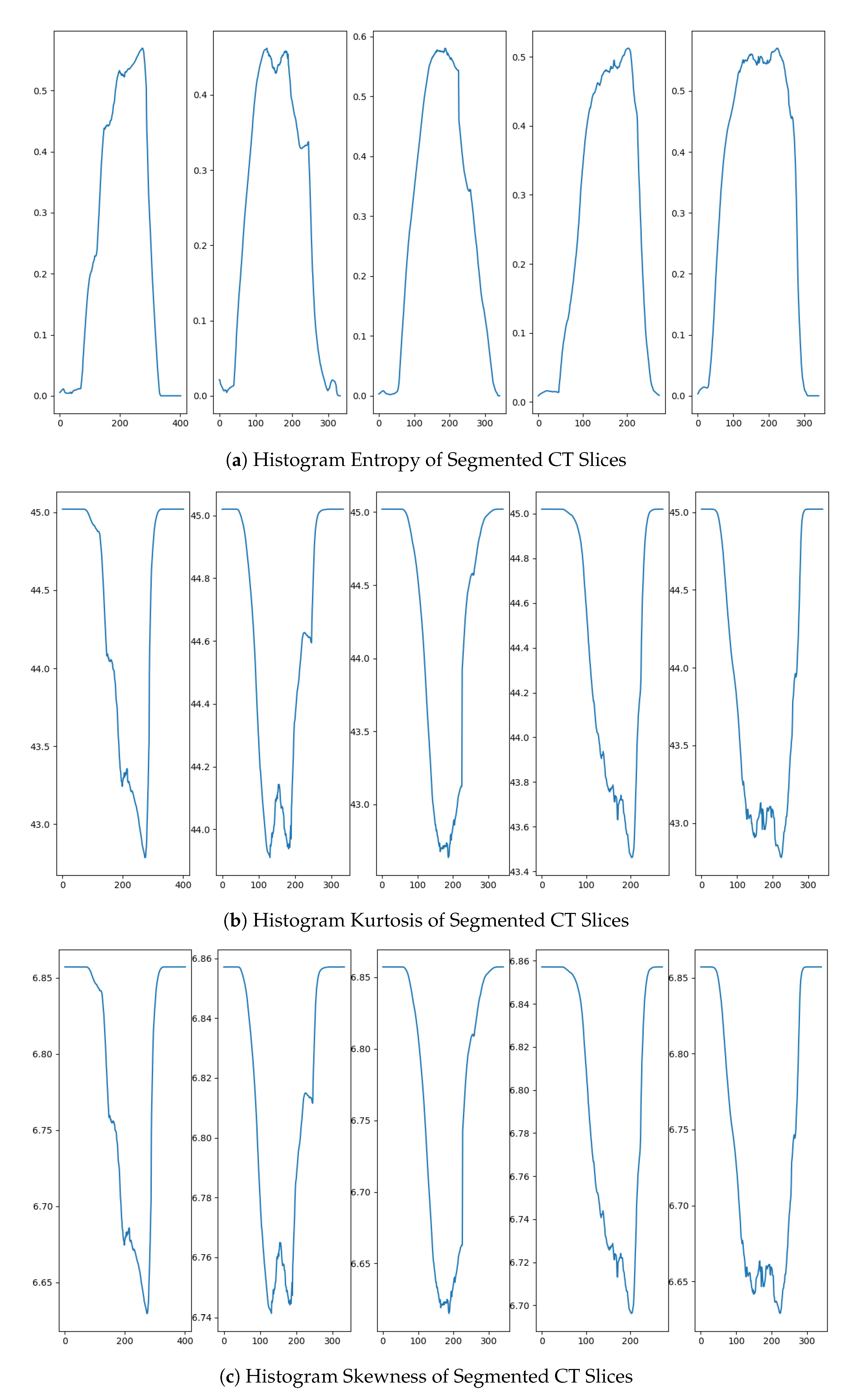
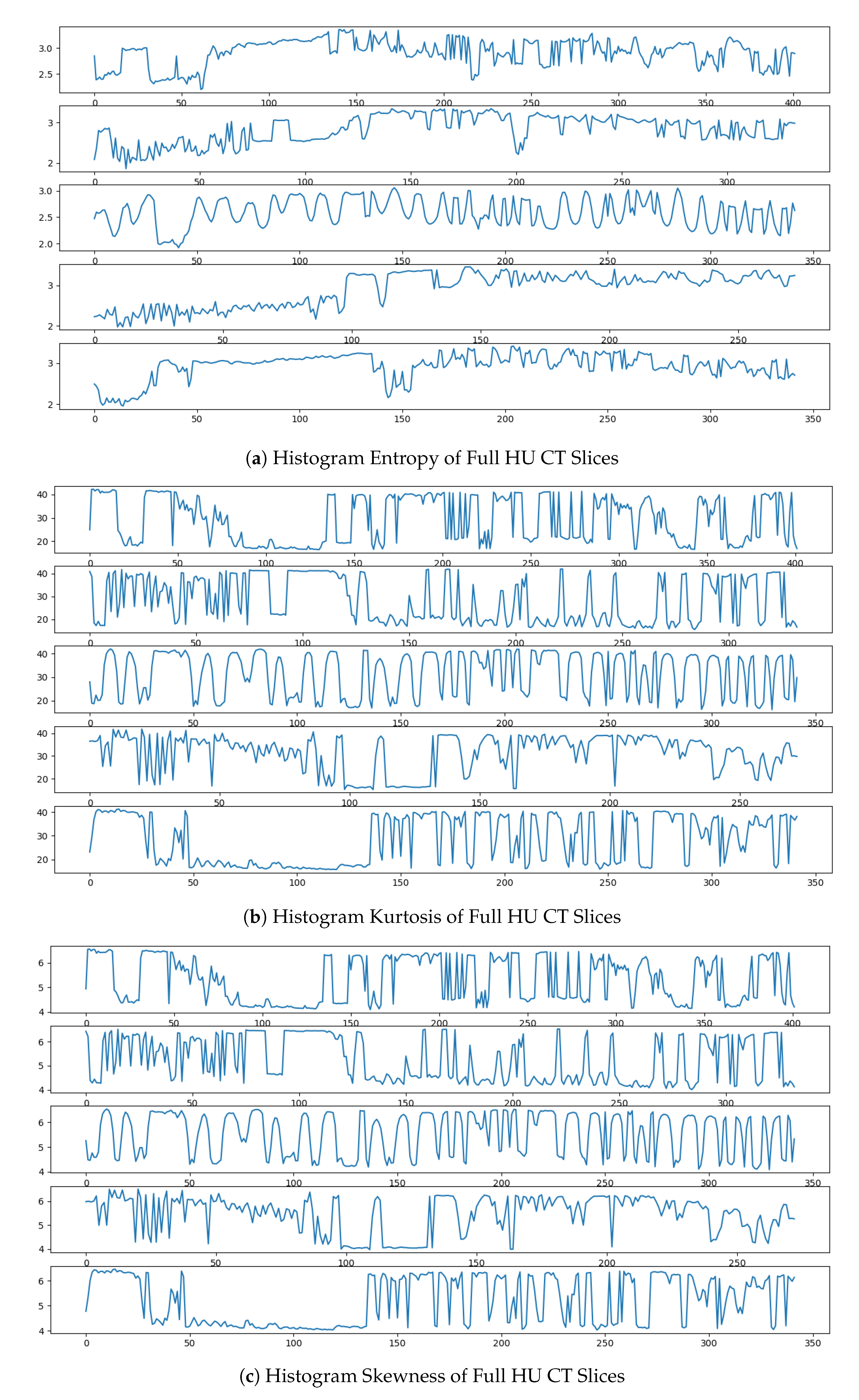
For Histogram-based features, three descriptive statistical measures are computed for each histogram. Histogram Entropy ($E{n}_H$) measuring the uncertainty and disagreement of the distribution is calculated according to the equation shown below. Kurtosis ($K_H$) and Skewness ($S{k}_H$) measures are calculated. Kurtosis ($K_H$) detect whether the data are heavy-tailed or light-tailed relative to a normal distribution. Skewness ($S{k}_H$) checks the lack of symmetry. The measures are evaluated given the following equations, where N is the number if bins, w is the bin width, $pr$ is the bin probability and $Ct$ is the bin count.

$$\begin{array}{cc}& E{n}_H=-{\sum }_{i=1}^{N}p{r}_{i}log(p{r}_i/w_i)\end{array}$$

(8)

$$\begin{array}{cc}& K_H={\sum }_{i=1}^N\frac{{(C{t}_i-\overline{C}t)}^4/N}{{\sigma }^4}\end{array}$$

(9)

$$\begin{array}{cc}& S{k}_H={\sum }_{i=1}^N\frac{{(C{t}_i-\overline{C}t)}^3/N}{{\sigma }^3}\end{array}$$

(10)

After feature extraction, a range of clustering algorithms, such as modified k-means variant [30], agglomerative [31], Spectral [32], and BIRCH [33] are applied to create different data partitions (clusters). The applied approach is outlined in Algorithm 1. Since there is substantial variability in the slices that are to be considered for selection or omission as shown in Figure 4, the targeted number of clusters to best partition the data cannot be determined beforehand. Therefore, the number of clusters fit for the data is verified experimentally. The quality of the clusters are evaluated to elect the partition of the best usability to DETECT-LC pipeline through well established clustering quality metrics.

Algorithm 1 Radiomics-based semi-supervised slice selection

1: procedureSS( $C{T}_s$) 2:     $\mathbf{for}\mathbf{each}SinC{T}_s$ 3:     $ApplyDICOMretrospectiveprocessing$ 4:     $PerformHU-basedlungparenchymasegmentationgeneratingbinarymask{S}_{LP}$ 5:     $\mathbf{end}\mathbf{for}$ 6:     $\mathbf{for}\mathbf{each}{S}_{LP}$ 7:     $GenerateHaralickTexturefeatures\mathit{ASM},\mathit{C},\mathit{SE},\mathit{H},\mathit{E}$ 8:     $GenerateHistogramTexturefeaturesE{n}_H,K_H,S{k}_H$ 9:     $GenerateFeatureVector:\mathit{ASM},\mathit{C},\mathit{SE},\mathit{H},\mathit{E},E{n}_H,K_H,S{k}_H$ 10:     $\mathbf{end}\mathbf{for}$ 11:     $Applyclustering:k-means,Agglomerative,BIRCH,andSpectralClustering$ 12:     $\mathbf{return}Outputclusters$ 13: end procedure

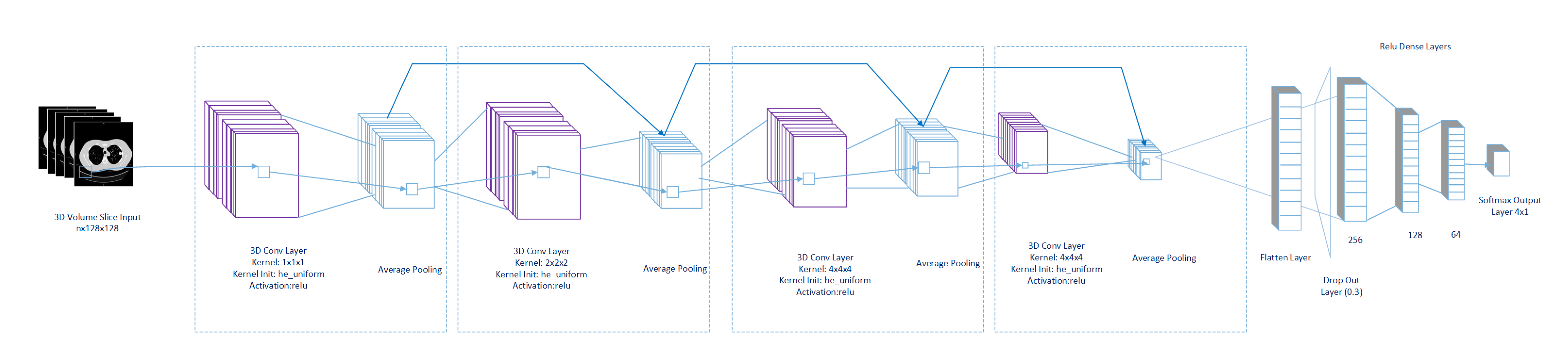
4.4. ALT-CNN-DENSE Net Architecture

After the selection phase, the slices are constructed into 3D volumes and input to the proposed ALT-CNN-DENSE Net model. The proposed architecture is illustrated in Figure 5, where it depicts the characterizing blocks of alternating convolution and average pooling layers followed by a drop out layer and multiple dense layers. The structure of the network architecture is detailed in

Table 2. ALT-CNN-DENSE Net Architecture Layers Description.

Layer	Output
conv3d (Conv3D)	(v, 40, 128, 128, 1)
average_pooling3d	(v, 20, 64, 128, 1)
conv3d_1 (Conv3D)	(v, 20, 64, 128, 8)
average_pooling3d_1	(v, 10, 32, 128, 8)
conv3d_2 (Conv3D)	(v, 10, 32, 128, 16)
average_pooling3d_2	(v, 5, 16, 128, 16)
conv3d_3 (Conv3D)	(v, 5, 16, 128, 32)
average_pooling3d_3	(v, 3, 8, 64, 32)
conv3d_4 (Conv3D)	(v, 3, 8, 64, 64)
average_pooling3d_4	(v, 2, 4, 32, 64)
conv3d_5 (Conv3D)	(v, 2, 4, 32, 128)
average_pooling3d_5	(v, 1, 2, 16, 128)
flatten (Flatten)	(v, 4096)
dropout (Dropout)	(v, 4096)
dense (Dense)	(v, 1024)
dense_1 (Dense)	(v, 256)
dense_2 (Dense)	(v, 128)
dense_3 (Dense)	(v, 64)
Output	(v, n)

v: varies with input volume.

. ALT-CNN-DENSE Net uses 3D kernels for the convolution process on the input CT volumes, which enables the extraction of both spatial and spectral features [34]. Such capability provides an advantage over 1D and 2D CNNs. However, this comes at the cost of increased complexity. Thus, the sequence of blocks of alternating convolution (CONV) and pooling layers are devised for dimensionality reduction and subsequent complexity moderation. Pooling eliminates redundant and irrelevant information reducing overfitting. Also, it provides spatial translation invariance [35]. In addition to the known advantages of pooling, the downsampling generates bird’s eye view feature maps for the following CONV layers. The generated feature maps aid the early detection of 3D primitives reducing the CNN depth. The CONV layers comprise different filter sizes to extract the multiscale inter-slices granule details in each volumetric input. The architecture has inherited the residual connectivity from RESNET. Average pooling layers as well as global average layer was taken from InceptionV3. Residual connections allow gradients to flow through a network directly, without passing through activation functions. At this point, the convolved features are passed between layers with the residual. This has the advantage to compensate any loss in the features between extensive mathematical calculations of layers as well as preserve spatial and temporal features in slices at the same time. Average pooling is used instead of Max pooling to guarantee that pixels with their surroundings relations are taken into consideration and not ignored. Average pooling maintains inter and intra-slices locality spatiotemporal information, unlike in Max Pooling where specific features are selected despite of location. The position of the tumor is critical for lung tumor phenotyping and cancer staging, which explains why average pooling gives higher performance with the problem considered here.

The flatten layer is added to convert the extracted features from the previous Convolution-AveragePooling (CNN-AVP) block to a 1D vector. The features vector is fed into a fully connected network of a set of dense layers. A drop out layer is added to reduce overfitting and improve generalization error. The deep dense layers concatenate the feature maps from all of the previous nodes and forward them to the following layers. New comprehensive feature maps are created from the fully connected dense network, which is expected to improve the CNN performance [36]. The softmax layer of this network outputs (n) classifications. To sum up, the developed architecture offers advantages of architecture depth reduction, extraction of both spatial and spectral features, generation of multiscale feature maps, reduced risk of overfitting and features reuse.

5. Results and Discussion

The experimental findings of each phase of $DETECT$-$LC$ pipeline are presented. First, the results of the preparation stage, including preprocessing, feature extraction and unsupervised slice selection steps are reported. After data preparation, the performance of ALT-CNN-DENSE Net is tested.

5.1. Experimental Tools and Setup

Preprocessing and slice selection are performed using pyRadiomics v3.1 and keras preprocessing packages, while ALT-CNN-DENSE Net implementation, training, testing and validation are done using Python language v3.7.6 with Keras package v2.3 (TensorFlow v2.1 backend). Also, numpy v1.18.4 and OpenCV v4.2.0 packages are used. Experiments are conducted on core i7, 2.21 GHz processor with 16 GB RAM and NIVIDIA TESLA v100-sxm2-16gb. Curves and diagrams have been created and exported using matplot and Microsoft Visio.

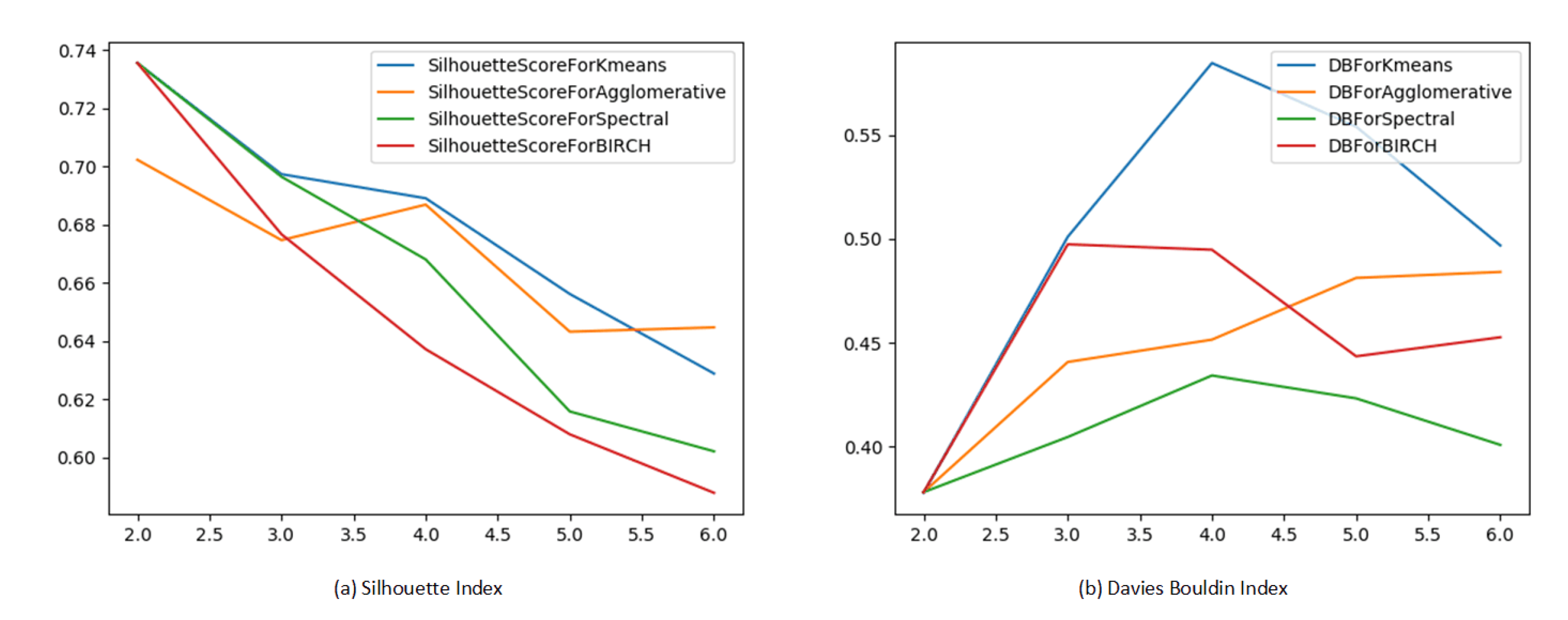
The performance of the simple HU-based segmentation approach is evaluated against the thoracic cavity segmentation masks provided with the datasets. Dice similarity coefficient [37] is used for segmentation evaluation. It quantifies the overlap between two binary segmentation masks, where a value of 0 indicates no overlap and a value of 1 indicates complete overlap. For the clustering-based slice selection phase, the quality of the produced partitions is evaluated by two well-established clustering evaluation indices. The performance metrics used are Silhouette index (Sil) and Davies Bouldin (DB) index [38], which measure the intra-clutser and inter-cluster distances. The purpose is to select the clusters with the highest compactness and best separability from the other clusters (i.e., higher Silhouette index and lower Davies Bouldin value). A range of cluster numbers are tested with the different clustering algorithms to determine the best suited algorithm and number of clusters based on Sil and DB values. Then, the appropriate number of clusters is affirmed through the elbow method [39].

All CNN architectures are trained from scratch using Adam optimizer with starting learning rate of 0.0001. ReLU activation is used to help overcome the vanishing gradient problem. The percentage splits of the datasets into training, validation and testing are 0.55, 0.15 and 0.3 respectively. Inputs are divided into batches of size 5. Validation accuracy and mean-squared-error are monitored for each epoch. In addition, the learning rate is reduced by almost a factor of 0.15 for every two consecutive epochs without improvement in validation. The best model is defined as having the maximum validation accuracy then it is stored and applied on the testing. Boot strapping with replacement is applied and the reported results represent the average of 10 runs. The performance of the CNN classification models is evaluated using four performance measures and confusion matrix [40]. The metrics are accuracy (Acc), sensitivity (Sn), F1-Score and AUC. Confusion matrices are displayed to show the classification distribution across class labels to aid the visualization of the pipeline performance.

5.2. Preparation Stage Results

Based on the adopted multilevel thresholding procedure, a binary mask is generated for each slice, as shown in Figure 6.

The mask images clearly outline the lung tissue in the middle lung slices and manifest a constant image for peripheral lung slices. The presented output manifest the success of the thresholding approach in generating segmentation masks for the lung tissue. Dice coefficient is calculated for the three datasets and the results are shown in

Table 3. HU-based segmentation evaluation using dice ($D_C$) coefficient on the TCIA NSCLC datasets.

Dataset	${\mathit{D}}_{\mathit{C}}$
NSCLC Radiomics (Lung 1)	0.79
NSCLC Radiomics-Genomics	0.85
NSCLC Radio-Genomics	0.89

. The achieved $D_C$ values presents acceptable performance as the recommended $D_C$ value for a good overlap is >0.700 according to Zijdenbos et al. [37]. Hence, the HU-based mask generation approach is considered satisfactory, especially that the masks are used solely for textural analysis and subsequent slice selection.

For each slice S, $ASM$, C, $SE$, H, E, $E{n}_H$, $K_H$ and $S{k}_H$ features are extracted from the full HU CT slices and their corresponding binary masks $S_{LP}$. In Figure 7, Haralick features values variation across slices of five patients are depicted. The diagrams elucidate that the features generated from the binary masks between peripheral slices and middle slices better differentiate discriminative vs non-discriminative features. For instance, $ASM$ takes a value of one for constant images denoting non-discriminative lung slices. Similarly, contrast feature C has a constant value of zero for all peripheral non-informative lung slices, while it varies with the middle informative lung slices. Histogram based features depict the same pattern, which is clear when comparing Figure 8 and Figure 9. Thus, the features extracted from the binary masks are the ones selected to be input to the clustering algorithm.

The performance of modified k-means variant [30], agglomerative [31], Spectral [32], and BIRCH [33] clustering is evaluated. Figure 10 shows the Sil index and DB index of each clustering algorithm varying with cluster number. Considering Sil index, k-means presents the best performance across all cluster numbers. While in terms of DB, it is equivalent to BIRCH clustering at two clusters. Nevertheless, k-means is employed for the purpose of slice selection for its intrinsic advantages such as scalability to large datasets and adaptiveness to data points cluster assignment [41].

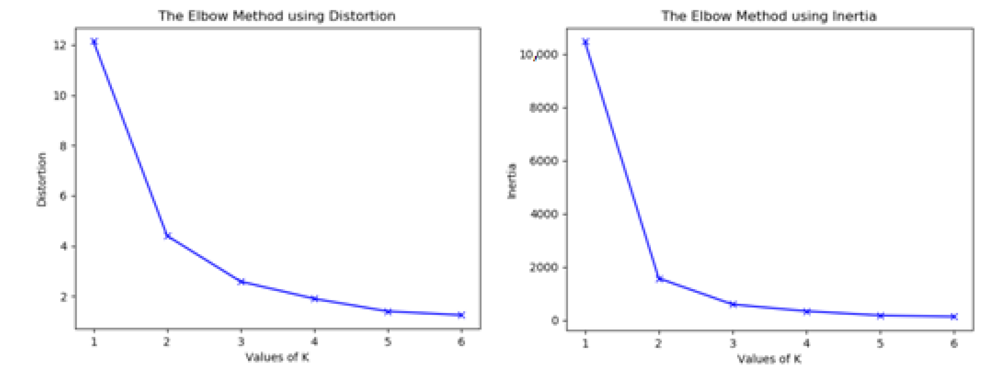
The best number of clusters is decided through the elbow method, as illustrated in Figure 11. From the shown diagrams, the optimum number of clusters can be chosen to be two or three. However, in view of the Sil and DB indices values in Figure 10, we opt to two clusters. The choice of two clusters also naturally corresponds to the open/closed lung partitions. Given the resultant clusters, the n slices nearest to the cluster centroid are selected per patient. The chosen slices are used to construct the 3D volumetric structures (nifti files), which are input to ALT-CNN-DENSE Net for training, validation and testing.

5.3. Voxel-Based Classification Results

The discriminating ability of the proposed ALT-CNN-DENSE Net and $DETECT$-$LC$ pipeline is assessed using two scenarios: NSCLC carcinoma subtypes classification (ADC, SCC and NOS) and lung cancer staging (I, II, IIIA and IIIB). The focus of this study is on ADC, SCC and NOS as they comprise 80% of the diagnosed subtypes [42] and are commonly available for all the study datasets. The described classifications are produced on NSCLC radiomics, NSCLC radiomics-genomics, and NSCLC radio-genomics datasets. Each dataset is split for training and testing purposes. The percentage split per class is around 55% for training, 15% for validation and around 30% for testing.

An ablation study is conducted to signify the contribution of ALT-CNN-DENSE Net in $DETECT$-$LC$ pipeline to the final classification output. Hence, the output of $DETECT$-$LC$ full pipeline is compared against our proposed radiomics preparatory stage (RPS) and off the shelf 3D ResNet-50 and Inception V3. The performance of ALT-CNN-DENSE Net is compared with RESNET-50 and Inception V3 due the inherent similarities between them. An additional experiment for NSCLC-Radiomics dataset is conducted, where a set of slices are statically selected with predefined indices. The slices are selected at the middle of the CT series depending on the size of the series. This approach is used instead of the proposed radiomics unsupervised approach to determine the value of the preparatory stage. The results of this experiment are reported as Static Selection (SS) + ALT-CNN-DENSE Net. NSCLC-Radiomics dataset is chosen for this experiment as it comprises the largest number of patients volumes and slices.

5.3.1. Lung Cancer Pathology Phenotyping

Pathology phenotyping is carried out on the three datasets separately and the results are reported accordingly in

Table 4. Lung Cancer Phenotyping Performance Evaluation on NSCLC Radiomics (Lung 1).

Model	Acc	Sn	F1-Score	AUC
SS + ALT-DENSE	0.60	0.61	0.62	0.41
RPS + ResNet-50	0.67	0.62	0.64	0.58
RPS + InceptionV3	0.89	0.7	0.81	0.71
$DETECT$-$LC$	0.96	0.93	0.93	0.83

,

Table 5. Lung Cancer Phenotyping Performance Evaluation on NSCLC Radiomics-Genomics.

Model	Acc	Sn	F1-Score	AUC
RPS + ResNet-50	0.67	0.62	0.64	0.58
RPS + InceptionV3	0.86	0.9	0.71	0.8
$DETECT$-$LC$	0.92	0.87	0.91	0.88

and

Table 6. Lung Cancer Phenotyping Performance Evaluation on NSCLC Radio Genomics.

Model	Acc	Sn	F1-Score	AUC
RPS + ResNet-50	0.82	0.73	0.71	0.51
RPS + InceptionV3	0.82	0.61	0.7	0.6
$DETECT$-$LC$	0.93	0.88	0.92	0.89

.

All the performance metrics in Table 4, Table 5 and Table 6 portray the superior performance of $DETECT$-$LC$, compared to SS+ALT-DENSE Net, RPS + ResNet-50 and RPS+ Inception V3 counterparts. The superior performance highlights the importance of each phase. $DETECT$-$LC$ achieves higher performance when compared to RPS + ResNet-50 on all datasets with a minimum difference of 0.11, 0.15 and 0.21 in terms of accuracy (Acc), sensitivity (Sn) and F1-score respectively on NSCLC Radio Genomics. The minimum AUC difference of 0.25 is on NSCLC Radiomics. A smaller improvement is attained against RPS + Inception V3; nevertheless it managed to score a minimum of 0.06, 0.2 and 0.08 improvement in terms of Acc, F1-score and AUC, respectively. As for the manual static slice selection comparison, an immense performance gap is observed where $DETECT$-$LC$ outperformed SS + ALT-DENSE Net with 0.29, 0.32, 0.31 and 0.42 gap for Acc, Sn, F1-score and AUC respectively. Another parameter worth noting in this experiment is training convergence time, as SS + ALT-DENSE Net recorded seven hours of training time against 48 min for $DETECT$-$LC$. These findings highlight the inability of ALT-DENSE Net to extract distinguishing features from the statically selected slices. This is due to the fact that they contain non-discriminative (closed) lung slices, which dramatically degrades the performance of ALT-CNN-DENSE Net.

$DETECT$-$LC$ is contrasted to state of the art studies, which experimented on the TCIA NSCLC datasets. Marentakis et al. [16], Chaunzwa et al. [15] and Khodbashki et al. [17] worked on NSCLC Radiomics dataset, whereas Yang et al. [18] studied the performance of their model on a merged dataset of NSCLC Radiomics, NSCLC Radiogenmoics and a private dataset from China Institute. The best results for these related studies are detailed in

Table 7. State of the Art Tumor Phenotyping Results on TCIA NSCLC Datasets.

Model	Acc	Sn	F1-Score	AUC
Chaunzwa et al. [15]	0.77	0.56	NA	0.71
Marentakis et al. [16]	0.74	0.81	0.76	0.78
Khodbashki et al. [17]	0.87	0.70	0.71	0.75
Yang et al. [18]	0.74	0.77	NA	0.78
$DETECT$-$L{C}_{avg}$	0.94	0.89	0.92	0.87

. $DETECT$-$LC$ outperforms the state of the art with an overall accuracy improvement ranging from 9 to 22%. Despite that Khodbashki et al. [17] manifest the best overall accuracy among the reported studies from the literature, it presented a sensitivity (Sn) value of 0.60 for ADC class. This was explained by the limited number of patients in ADC class; however, $DETECT$-$LC$ managed to attain a Sn of 0.83 on the same class. When comparing the average performance of $DETECT$-$LC$ on the three datasets to the state of the art, it is found that $DETECT$-$LC$ surpasses them with a minimum of 0.07, 0.08, 0.16 and 0.09 of Acc, Sn, F1-Score and AUC, respectively.

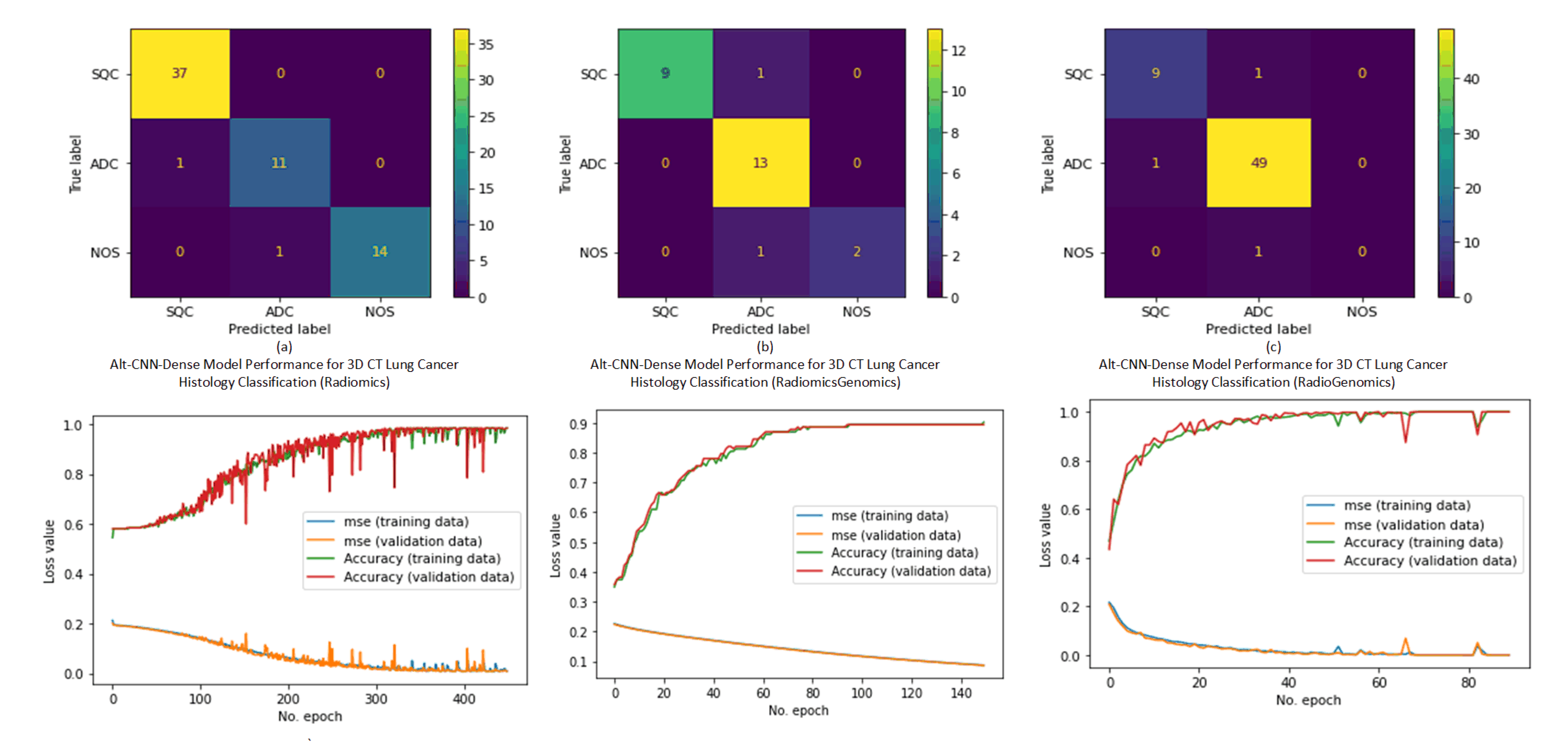
The confusion matrices of sample runs are outlined in Figure 12. The confusion matrices and the reported performance metrics show comparable performance across the three datasets. Moreover, the learning curves show minor differences between the training and validation curves, ruling out the possibility of overfitting.

5.3.2. Lung Cancer Staging

Similar results are realized with the staging scenario as shown in

Table 8. Lung Cancer Staging Performance Evaluation on NSCLC Radiomics (Lung 1).

Model	Acc	Sn	F1-Score	AUC
SS + ALT-DENSE Net	0.51	0.54	0.53	0.41
RPS + ResNet-50	0.56	0.59	0.57	0.47
RPS + InceptionV3	0.8	0.6	0.77	0.52
$DETECT$-$LC$	0.97	0.89	0.96	0.75

,

Table 9. Lung Cancer Staging Performance Evaluation on NSCLC Radiomics-Genomics.

Model	Acc	Sn	F1-Score	AUC
RPS + ResNet-50	0.66	0.65	0.52	0.41
RPS + InceptionV3	0.77	0.5	0.62	0.5
$DETECT$-$LC$	0.91	0.88	0.95	0.85

and

Table 10. Lung Cancer Staging Performance Evaluation on NSCLC Radio Genomics.

Model	Acc	Sn	F1-Score	AUC
RPS + ResNet-50	0.72	0.67	0.62	0.51
RPS + InceptionV3	0.83	0.57	0.61	0.55
$DETECT$-$LC$	0.93	0.88	0.92	0.84

. However, the performance measures of SS + ALT-DENSE and RPS+ResNet-50 indicate lower performance compared to the phenotyping scenario. Such a finding may be attributed to the fact that the data is stratified into four classes instead of three. On average, compared to RPS + ResNet-50 and RPS+ Inception V3 on the three datasets, $DETECT$-$LC$ records higher performance. The differences reached 0.29, 0.25, 0.37 and 0.35 in terms of Acc, Sn, F1-score and AUC, respectively against RPS + ResNet-50. Also, it achieves higher performance compared to RPS+ Inception V3 with 0.14, 0.38, 0.33 and 0.35 on the Radiomics-Genomics dataset.

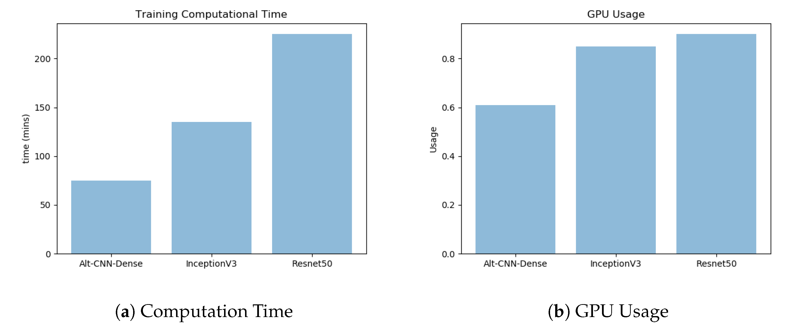
Other performance aspects that are noted are the model building and training time together with the GPU usage. Figure 13 shows the enhanced performance of ALT-CNN-DENSE Net given both performance aspects. The improvement can be attributed to the reduced architecture depth resulting from the successive early pooling layers combined with the residuals connections.

Table 11. State of the Art Staging Results on TCIA NSCLC Datasets.

Model	Acc	Sn	F1-Score	AUC
Moitra et al. [22]	0.87	NA	NA	NA
Choi et al. [20]	0.86	0.80	NA	0.82
Paing et al. [21]	0.91	0.77	0.80	0.85
$DETECT$-$L{C}_{avg}$	0.94	0.88	0.94	0.81

sketches the performance of the related studies applied on TCIA NSCLC Datasets and $DETECT$-$LC$ average staging results. Moitra et al. [22] performed TNM staging on NSCLC Radiogenomics dataset. Choi et al. [20] used NSCLC Radiogenomics and NSCLC Radiomics-Genomics datasets as training and validation sets for binary staging, whereas Paing et al. [21] experimented with the three datasets for seven classes T-staging only. The results of Paing et al. [21] were provided as collective averages. Although $DETECT$-$LC$ results cannot be directly compared with those of Choi et al. [20] and Paing et al. [21] due to the difference in staging approach, their results are reported for completeness and to give a clear estimate of $DETECT$-$LC$ performance. For instance, despite the simplified binary staging approach of Choi et al. [20], $DETECT$-$LC$ managed to attain higher performance metrics. Compared to Moitra et al. [22] on NSCLC Radiogenomics dataset, $DETECT$-$LC$ surpassed it with 7% in Acc. For staging results, $DETECT$-$LC$ average performance outperforms the next higher model with 0.03 of Acc, 0.08 of Sn and 0.14 of F1-Score.

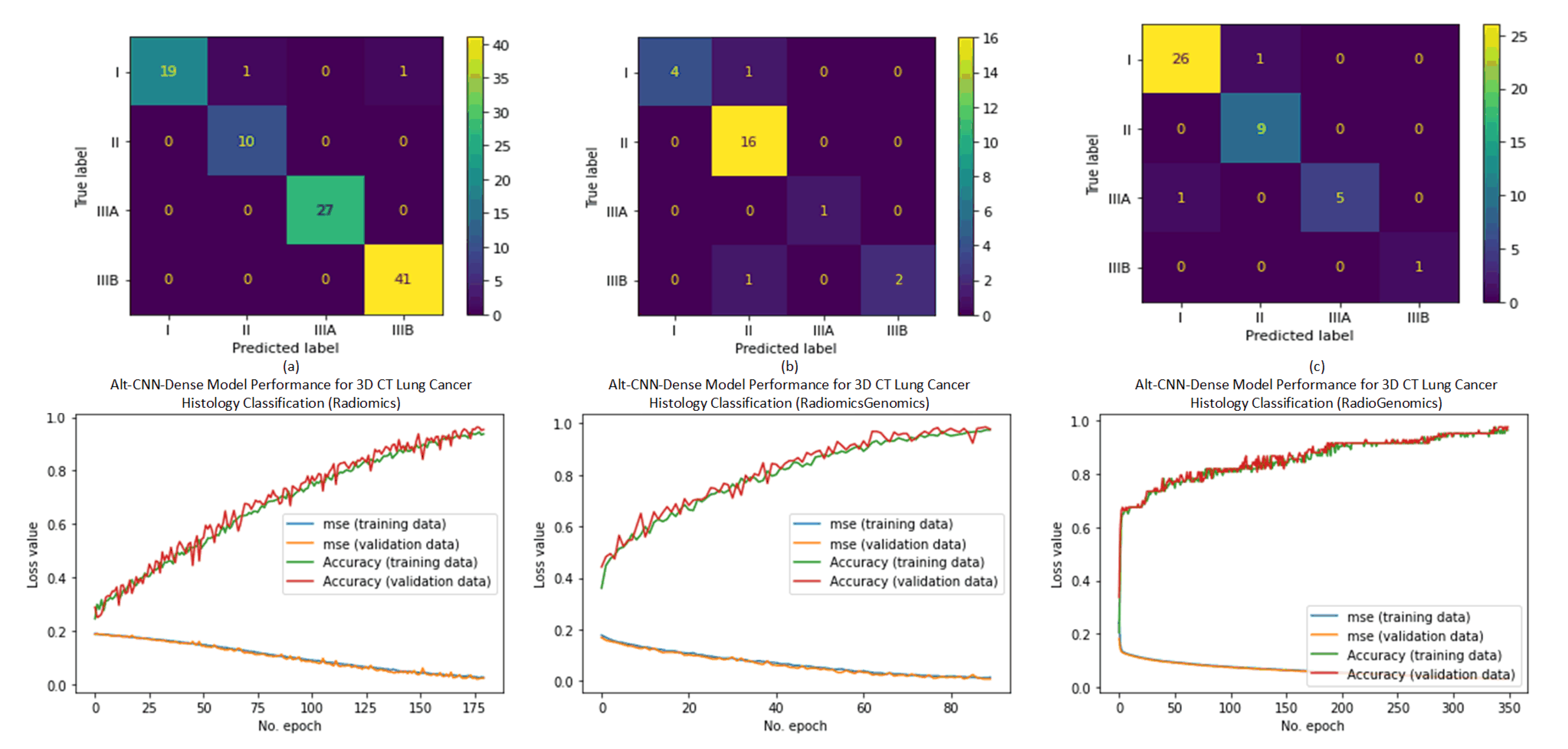
In Figure 14, the sample confusion matrices elucidate the ability of ALT-CNN-DENSE Net to discriminate minority classes. It is particularly evident with Stage IIIB in Radiogenomics and Radiomics-Genomics datasets, where the number of training and testing samples is challenging. This proves that the ALT-CNN-DENSE Net can handle imbalanced data with highly skewed distributions. The learning curves exhibit a similar pattern to phenotyping curves.

To sum up, our proposed model manifested acceptable performance compared to the state of the art, which illustrates its success in handling the problem considered here, as well as other engineering problems [43,44,45,46].

6. Conclusions

In this study, a multistage computational model $DETECT$-$LC$ is proposed for lung cancer tumor phenotyping and staging based on 3D CT volumes. $DETECT$-$LC$ handles the challenge of choosing discriminative CT slices for constructing 3D volumes. Haralick radiomics and k-means clustering are used for this purpose. Then, ALT-CNN-DENSE Net is developed for distinguishing the pathology and stage classes. For phenotyping, $DETECT$-$LC$ gets a minimum accuracy of 0.92, sensitivity of 0.87, F1-score of 0.91 and AuC of 0.88 with the smallest dataset NSCLC Radiomics-Genomics. Similarly for staging, the least results are obtained with NSCLC Radiomics-Genomics dataset with values 0.91, 0.88, 0.95 and 0.85 for Acc, Sn, F1-score and AuC, respectively. $DETECT$-$LC$ shows a robust consistent performance across the three experimented TCIA NSCLC datasets with minor differences in performance. Also, the performance assessment conveyed the capacity of the pipeline to classify small highly imbalanced datasets exceeding the performance of the state of the art. Generally, $DETECT$-$LC$ is shown to have superior performance relative to various similar solutions. Hence, $DETECT$-$LC$ can provide an ample solution to different recognition tasks. As future work, data integration between different organs’ CT will be considered to detect metastasis. Also, the staging study can be enlarged to include Stage IV. Also, other data types can be integrated with CT, such as genomes, in order to build a Radio-Genomic model and improve the diagnosis results. In addition, the model can be embedded in a user-friendly desktop application to aid doctors and non-medical experts in analyzing Lung CTs to expand its usability.