Optimal Robust LQI Controller Design for Z-Source Inverters

Abstract

This paper investigates the linear quadratic integral (LQI)-based control of Z-source inverters in the presence of uncertainties such as parameter perturbation, unmodeled dynamics, and load disturbances. These uncertainties, which are naturally available in any power system, have a profound impact on the performance of power inverters and may lead to a performance degradation or even an instability of the system. A novel robust LQI-based design procedure is presented to preserve the performance of the inverter against uncertainties while a proper level of disturbance rejection is satisfied. The stability robustness of the system is also studied on the basis of the maximum sensitivity specification. Moreover, the bat algorithm is adopted to optimize the weighting matrices. Simulation results confirm the effectiveness of the proposed controller in terms of performance and robustness.

1. Introduction

The substantial progress of modern power inverters is well underway for the penetration of renewable energy sources into power systems and many other industrial applications [1]. The Impedance Source Inverters (also called Z-Source Inverters or ZSIs) form a class of high-performance, highly reliable, and highly efficient yet low-cost inverters equipped with an X-shaped impedance circuit that enables shoot-through state [2,3]. Hence, they can overcome the limitations of traditional inverters and fulfill both buck and boost capability in a single-stage topology without the necessity for any kind of delays [4,5]. Therefore, the output voltage can be adjusted freely to provide a wider voltage gain range without any additional cost or distortion [6]. Additionally, besides the advent and advance of new pulse width modulation (PWM) methods, all the traditional PWM schemes can be used to drive the inverter bridge and control the ZSIs [7]. These interesting features have paved the ZSI’s way for penetrating into different industrial applications such as photovoltaic power generation [8], wind energy [9], electric vehicles (EV) [10], motor drive [11], and battery energy storage [12].

Multiple new versions of ZSIs are proposed in the literature to improve their performance and consolidate their position in the industry, which can be classified into four general categories: constant boost ratio, improved boost ratio, multilevel and multiplex, and parameter optimization topologies. The first category can be further subdivided into six classes:

• Basic topology
• Improved topologies
• Neutral point topologies
• Reduced leakage current topologies
• Quasi topologies
• Other topologies

The second category can be further subcategorized into four classes:

• Switched components topologies
• Tapped inductor topologies
• Cascaded quasi topologies
• Coupled inductor topologies (such as the T-source inverter, gamma-source inverter, Y-source inverter (YSI), improved YSI, $\Delta$-source inverter, trans-quasi ZSI, improved trans-quasi ZSI, and transformer ZSI)

Multilevel topologies consist of three, four, or more-level cascaded and dual-input or dual-output topologies. Finally, parameter optimization topologies involve high-frequency transformer-isolated ZSI, inductor ZSI, extended quasi YSI, low dc-link voltage spikes YSI, and other optimized topologies.

The ZSI possesses a non-minimum phase characteristic with a real right-half plane zero, which imposes special constraints on the performance of the control system [13]. It is well known that real non-minimum phase zeros lead to an undershoot and also overshoot in the transient response, increase the harmonic distortions, and jeopardize system stability, thereby making the control problem complicated. Besides, parameter scanning of the pole-zero map reveals that altering system parameters cannot completely eliminate the non-minimum phase zeros [14]. Hence, in contrast with two-stage inverters, the ZSI closed-loop control is not an easy task. Over recent years, a variety of single-loop, dual-loop, and nonlinear control actions have been successfully applied generally using state-space averaging or small-signal modeling techniques [15]. The single-loop methods commonly employ the feedback by the input voltage [15], capacitor voltage [16], or dc-link voltage [17] to the closed-loop control of ZSIs through traditional PI controllers. A PID controller is proposed in [18] to provide a constant capacitor voltage with an excellent transient performance besides enhanced disturbance rejection. Variations of the dc-link voltage caused can be further suppressed by using dual-loop methods with an additional PI control loop [19]. Finally, nonlinear control approaches, for instance, the neural network control [20], sliding mode control [21,22], fuzzy control [23], model predictive control [24], and adaptive control [25] have also been presented.

Given the uncertain and time-varying nature of some regulator parameters such as load or storage elements, it is of vital importance to seek for control methods which can deal efficiently with performance requirements, disturbances, and uncertainties. Conventional controllers have a simple and efficient structure but are still not robust against perturbations. The robust control methods, such as $H_{\infty }$ [26], $\mu$-synthesis [27], quantitative feedback theory [28], linear matrix inequality (LMI)-based approaches [29], and sliding mode control [30] have been applied to overcome both structured and unstructured uncertainties of different converters. Among these robust control techniques, the linear quadratic integral (LQI)-based control offers optimal control for uncertain systems with given weighting matrices $\mathcal{D}$ and $\mathcal{R}$ [31].

To the best of the authors’ knowledge, it can be concluded from the literature that there is no published work addressing the LQI-based control of the ZSIs. Hence, considering the uncertain and non-minimum phase nature of the system, an LQI-based robust controller is designed to achieve an optimal robust performance against uncertainties and load disturbances in which controller parameters are tuned using the bat optimization algorithm. Most importantly, the stability robustness of the proposed method is also investigated on the basis of the maximum sensitivity specification. By considering the inverter in different operating states and using state-space averaging (SSA), a non-minimum phase model with a right-hand-plane real zero is derived for the inverter. To fairly assess the performance obtained by the proposed controller, the results are compared with those obtained through PI and state feedback (SF) controllers within dual-loop schemes. The simulation results reveal that despite the perturbed condition and non-minimum phase issue, the synthesized controller preserves no overshoot and less undershoot transient response with an acceptable disturbance rejection.

The rest of this paper is organized as follows: circuit analysis and the uncertain model of the inverter are represented in Section 2. Section 3 explicates the synthesis procedure of the proposed controller. Simulation results are presented in Section 4. Eventually, conclusions are summarized in Section 5.

2. Circuit Analysis

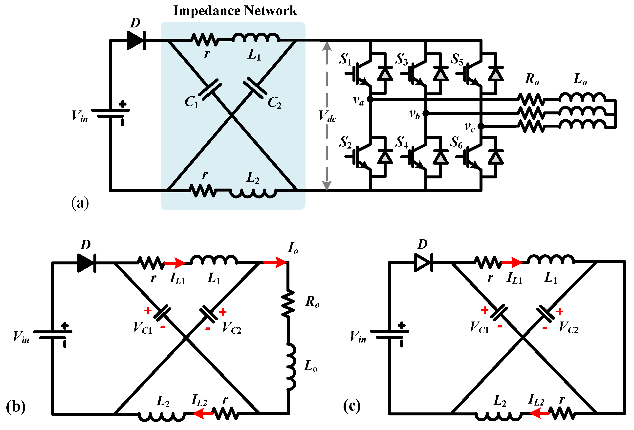
Figure 1a illustrates a three-phase voltage-fed ZSI consisting of power source, impedance network, switches, and AC load. The embedded X-shape network with two split inductors and capacitors adds an additional state to ZSIs and enables ZSIs to boost output voltage by changing the shoot-through duty cycle. Figure 1 depicts the topology of a ZSI in different switching states: the non-shoot-through mode (including six active modes when the DC voltage is impressed across the three-phase load and two conventional zero modes when the load terminals are shorted through either the lower or upper three switching devices, respectively) and shoot-through mode, during which the load terminals are shorted in seven different ways by any phase, with combinations of any two-phase legs and all three-phase legs. All these cases can be modeled mathematically using three state variables ($\mathrm{x}$): the inductor current in the impedance network $i_L$, the capacitor voltage in the impedance network $v_C$, and the output current $i_o$, i.e., $\mathrm{x}={[i_L,v_C,i_o]}^T$. $R_o$ and $L_o$ model the inverter load, while r denotes the parasitic resistance of the inductors. Due to the symmetrical structure of the impedance network ($C_1=C_2=C$, $L_1=L_2=L$), it is obvious that $v_{C1}=v_{C2}=v_C$ and $i_{L1}=i_{L2}=i_L$.

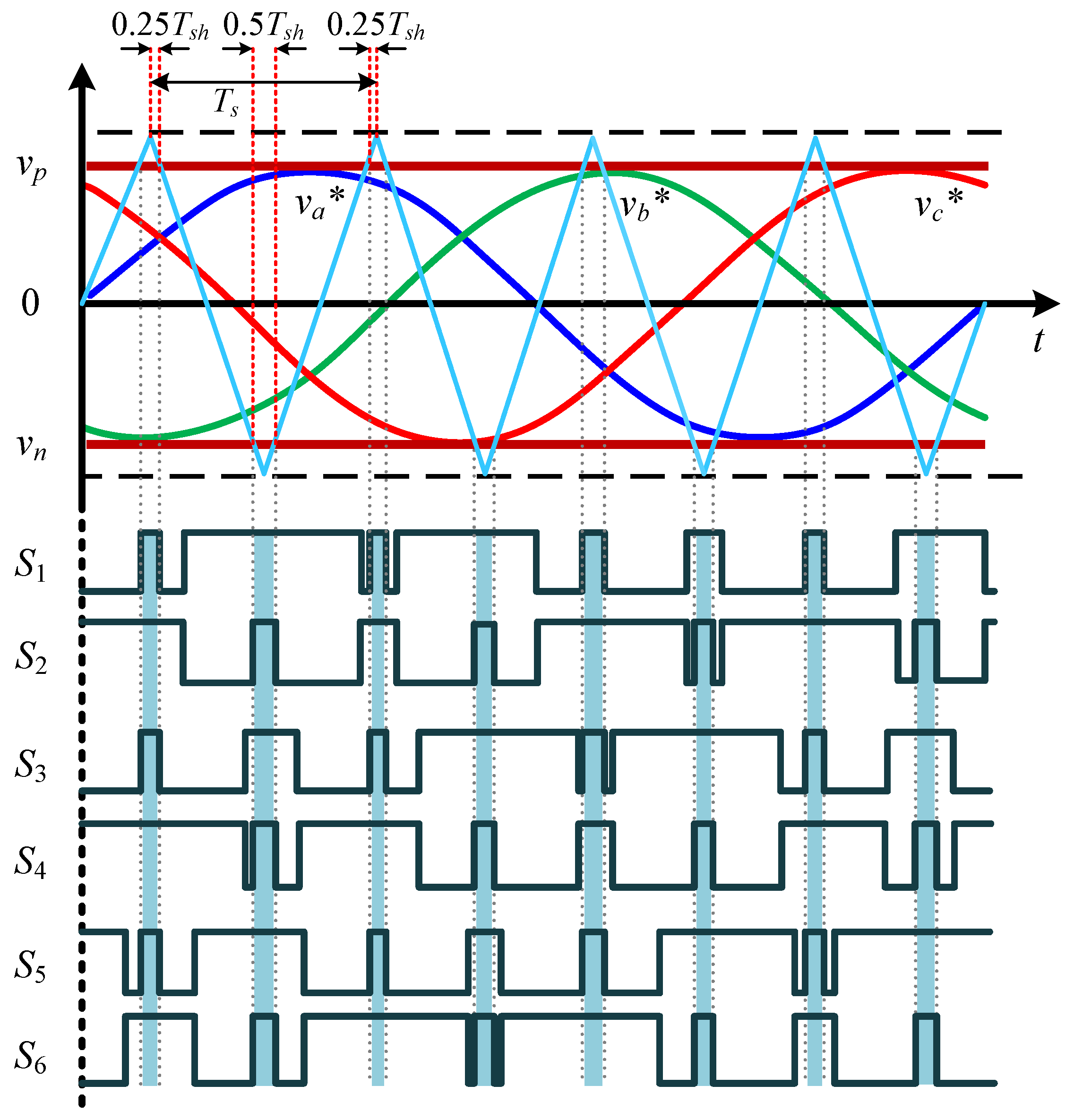
The shoot-through mode is inserted only into the zero states, whereas the active states remain unchanged, and hence the AC output voltage of the inverter remains similar to a traditional inverter besides the traditional PWM techniques can be adopted with slight modification to the zero states. Figure 2 describes the simple boost PWM modulation method, where the shoot-through zero vectors are evenly allocated into each phase without changing the total zero-vector time interval. Thus, the active-vector time is unchanged while the dc-link voltage is enhanced because of the introduction of shoot-through zero vectors. Here, $f=1/T_s$ denotes the switching frequency in which $T_s=T_n$ (non-shoot-through interval)$+T_{sh}$ (shoot-through interval), and the ratio $d=T_{sh}/(T_{sh}+T_n)$ is called the shoot-through duty cycle.

2.1. Non-Shoot-Through Mode

Figure 1b depicts the non-shoot-through mode, during which the inductors and input source transfer energy to the capacitors and load. The bridge can be seen as an equivalent current source (with zero current flowing in the zero mode). It can be mathematically expressed by the state space model expressed in (1).

$$\dot{\mathrm{x}}=\underset{A_n}{\underbrace{\left[\begin{array}{ccc}-\frac{r}{L}& -\frac{1}{L}& 0\\ \frac{1}{C}& 0& -\frac{1}{C}\\ 0& \frac{2}{L_o}& -\frac{R_o}{L_o}\end{array}\right]}}\mathrm{x}+\underset{B_n}{\underbrace{\left[\begin{array}{c}\frac{1}{L}\\ 0\\ -\frac{1}{L_o}\end{array}\right]}}{V}_{in}$$

(1)

In this mode, voltages across inductors and the dc-link are $V_L=V_{in}-V_C$ and $V_{dc}=V_C-V_L=2V_C-V_{in}$, respectively. In this mode, the duty cycle is equal to $1-d$.

2.2. Shoot-Through Mode

In this mode, as shown in Figure 1c, the output terminals of the inverter are shorted by a combination of upper and lower switches. During this mode, the diode is reversely biased, no voltage appears across the load and inductors are charged by the energy already stored in the capacitor. The boosting capability of the inverter is in fact due to this energy transfer according to the shoot-through duty ratio. In this mode, voltages across inductors and the dc-link are $V_L=V_C$ and $V_{dc}=0$, respectively. The state space equation of this mode can be written as (2).

$$\dot{\mathrm{x}}=\underset{A_{sh}}{\underbrace{\left[\begin{array}{ccc}-\frac{r}{L}& \frac{1}{L}& 0\\ -\frac{1}{C}& 0& 0\\ 0& 0& -\frac{R_o}{L_o}\end{array}\right]}}\mathrm{x}.$$

(2)

This equation does not have the term $B_{sh}\mathrm{u}$ because the inverse bias of the diode in Figure 1c results in $B_{sh}=0$. In this mode, the duty cycle is equal to d.

By using the SSA method, the overall state space equation can be computed as given by (3). Then, substituting (1) and (2) in (3) yields (4).

$$\dot{\mathrm{x}}=(A_n\times (1-d)+A_{sh}\times d)\mathrm{x}+(B_n\times (1-d)+B_{sh}\times d)V_{in}$$

(3)

$$\dot{\mathrm{x}}=\left[\begin{array}{ccc}-\frac{r}{L}& \frac{2d-1}{L}& 0\\ -\frac{2d-1}{C}& 0& -\frac{1-d}{C}\\ 0& \frac{2(1-d)}{C}& -\frac{R_o}{L_o}\end{array}\right]\mathrm{x}+\left[\begin{array}{c}\frac{1-d}{L}\\ 0\\ -\frac{1-d}{L_o}\end{array}\right]V_{in}.$$

(4)

By ignoring the parasitic resistances of inductors, i.e., $r=0$, the first row of (4) in the steady-state, $\dot{\mathrm{x}}=0$, gives (5).

$$V_C=\frac{1-D}{1-2D}{V}_{in}$$

(5)

where, D is the steady-state value of d. Therefore, the average voltage across dc-link can be calculated as (6).

$$V_{dc}=(1-D)\times (2V_C-V_{in})+D\times 0=\frac{1-D}{1-2D}{V}_{in}.$$

(6)

On the other hand, using Equation (5), the peak dc-link voltage can be expressed as (7).

$$v_{dc}=2V_C-V_{in}=\frac{1}{1-2D}{V}_{in}=B{V}_{in}$$

(7)

which means that the dc-link voltage is the boosted version of $V_{in}$ with $B=1/(1-2D)$ as the boosting factor. On the basis of (7), the peak output voltage of the ZSI can be reached as (8).

$$v_{ac}=M\frac{v_{dc}}{2}=MB\frac{V_{in}}{2}$$

(8)

where M denotes the modulation index. Hence, contrary to traditional inverters, the ZSI can buck-boost voltage to a desired level by offering an extra adjustable parameter, i.e., the boosting factor B.

2.3. Small Signal Model

The SSA method is known as a powerful tool, which provides a simple yet precise model for the small signal analysis of inverters [6,7]. Applying small signal perturbation for a given equilibrium point ($I_L$, $V_C$, $I_o$, D, M) and using the SSA model given by (4) yields (9),

$$\frac{d}{dt}\left[\begin{array}{c}{\widehat{i}}_L\\ {\widehat{v}}_C\\ {\widehat{i}}_o\end{array}\right]=\left[\begin{array}{ccc}-\frac{r}{L}& \frac{2(D+\widehat{d})-1}{L}& 0\\ -\frac{2(D+\widehat{d})-1}{C}& 0& -\frac{1-(D+\widehat{d})}{C}\\ 0& \frac{2(1-(D+\widehat{d}))}{L_o}& -\frac{R_o}{L_o}\end{array}\right]\left[\begin{array}{c}{I}_L+{\widehat{i}}_L\\ V_C+{\widehat{v}}_C\\ I_o+{\widehat{i}}_o\end{array}\right]+\left[\begin{array}{c}\frac{1-(D+\widehat{d})}{L}\\ 0\\ -\frac{1-(D+\widehat{d})}{L_o}\end{array}\right]V_{in}$$

(9)

where ${\widehat{i}}_L$, ${\widehat{v}}_C$, ${\widehat{i}}_o$ and $\widehat{d}$ are perturbations of state and control variables. Assuming the steady-state and removing second order terms, (9) can be simplified as given by (10).

$$\frac{d}{dt}\left[\begin{array}{c}{\widehat{i}}_L\\ {\widehat{v}}_C\\ {\widehat{i}}_o\end{array}\right]=\left[\begin{array}{ccc}-\frac{r}{L}& \frac{2D-1}{L}& 0\\ -\frac{2D-1}{C}& 0& -\frac{1-D}{C}\\ 0& \frac{2(1-D)}{L_o}& -\frac{R_o}{L_o}\end{array}\right]\left[\begin{array}{c}{\widehat{i}}_L\\ {\widehat{v}}_C\\ {\widehat{i}}_o\end{array}\right]+\left[\begin{array}{c}\frac{2V_C-V_{in}}{L}\\ \frac{I_o-2I_L}{C}\\ \frac{2V_C-V_{in}}{L_o}\end{array}\right]\widehat{d}$$

(10)

By solving (10) using Laplace transforms, the transfer functions at any given operating point can be obtained. For instance, the transfer functions of voltage across the capacitors to the shoot through the duty ratio can be obtained as given by (11), where $K_1=I_o-2I_L$ and $K_2=2V_C-V_{in}$.

$$\frac{{\widehat{v}}_C}{\widehat{d}}=\frac{K_{1}L{L}_o{s}^2+\left[K_1(L{R}_o+L_{o}r)+K_2(1-2D)L_o+K_2(1-D)L\right]s+K_{1}r{R}_o+K_2(1-2D)R_o+K_2(1-D)r}{CL{L}_o{s}^3+C(R_{o}L+r{L}_o)s^2+(Cr{R}_o+{(2D-1)}^2{L}_o+2{(1-D)}^{2}L)s+{(2D-1)}^2{R}_o+2{(1-D)}^{2}r}$$

(11)

As can be readily seen from (11), by applying the appropriate changes to the shoot-through duty cycle, d, the capacitor voltage can be regulated according to the connected load.

2.4. Extended Model

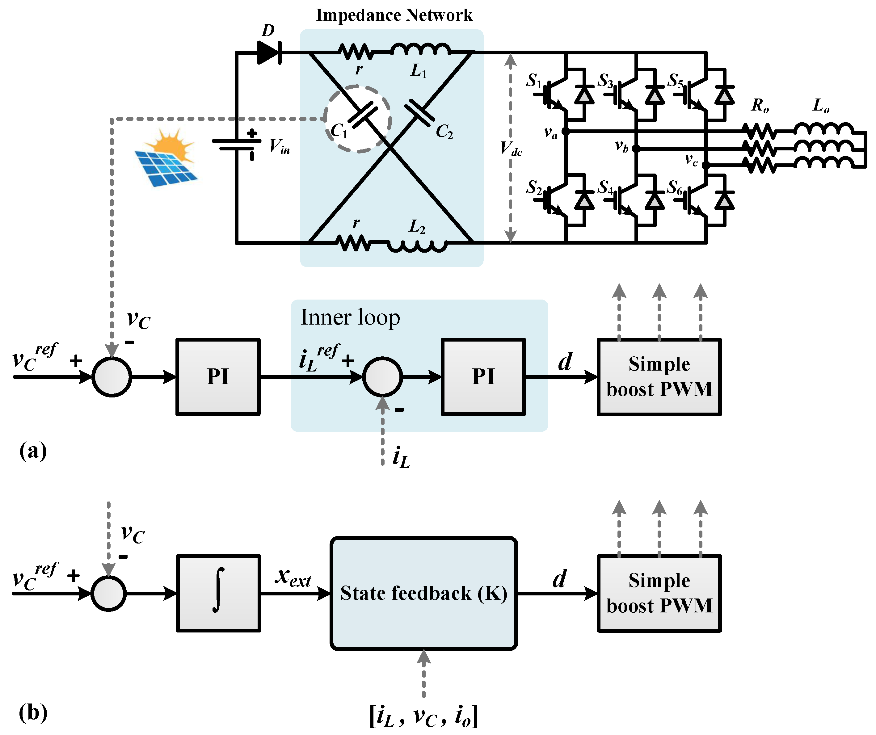
There exist several closed-loop techniques, either single or dual loops, to control the output voltage of a ZSI around a value, so as to achieve a near stable voltage. While the single-loop control causes fluctuation for the peak voltage across the dc-link in response to the source voltage fluctuations, as depicted in Figure 3a, an inner current loop is embedded within dual loop control systems to not only stabilize the peak voltage across the dc-link but realize a fast response as well. As depicted in Figure 3b, a similar approach can be adopted to the SF by introducing an integrator as the outer loop. The additional integral state is a requisite for the zero steady-state error and the regulated output of the system.

Herein, because of the simplicity in measurement, voltage across the capacitors is chosen as the control variable to control the dc-link voltage. To make sure that the capacitor voltage is controlled to the desired values, as shown in Figure 3b, another state, $x_{ext}$, is defined as the integral of the difference between the reference voltage and the capacitor voltage, as given by (12).

$$x_{ext}={\int }_0^t(v_C^{ref}-v_C)d\tau .$$

(12)

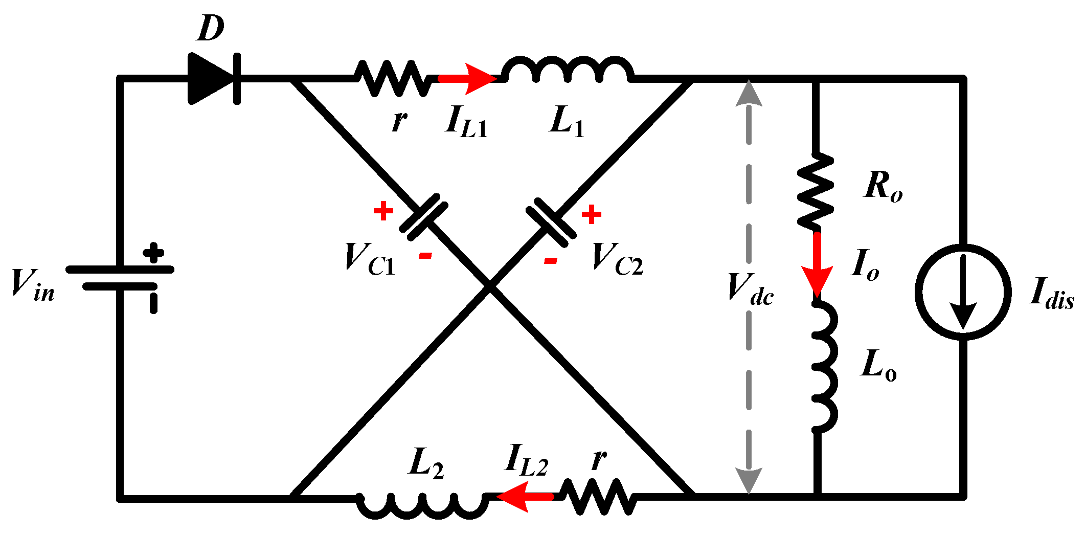
Furthermore, as shown in Figure 4, the disturbance vector in load $w\left(t\right)$ is modeled as an output current source $I_{dis}$. Therefore, the overall system equations can be modified as (13).

$$\left\{\begin{array}{c}\dot{\mathrm{x}}\left(t\right)=A_{tot}\mathrm{x}\left(t\right)+B_{u}u\left(t\right)+B_{w}w\left(t\right)+B_{ref}{v}_C^{ref}\hfill \\ \mathrm{y}\left(t\right)=C\mathrm{x}\left(t\right)+D_{u}u\left(t\right)+D_{w}w\left(t\right)\hfill \end{array}\right.$$

(13)

where $C=[0,1,0,0]$, $D_u=0$, $D_w=0$, $w\left(t\right)=I_{dis}\left(t\right)$ and $u\left(t\right)=d$ while $A_{tot}$, $B_u$, $B_w$ and $B_{ref}$ are expressed by (14). The capacitor voltage is considered as the controlled output $y\left(t\right)$ whose response has to fulfill the control requirements.

$$A_{tot}=\left[\begin{array}{cccc}-\frac{r}{L}& \frac{2D-1}{L}& 0& 0\\ -\frac{2D-1}{C}& 0& -\frac{1-D}{C}& 0\\ 0& \frac{2(1-D)}{L_o}& -\frac{R_o}{L_o}& 0\\ 0& -1& 0& 0\end{array}\right],B_u=\left[\begin{array}{c}\frac{2V_C-V_{in}}{L}\\ \frac{I_o-2I_L}{C}\\ \frac{2V_C-V_{in}}{L_o}\\ 0\end{array}\right],B_w=\left[\begin{array}{c}0\\ -\frac{1-D}{C}\\ 0\\ 0\end{array}\right]\mathrm{and}{B}_{ref}=\left[\begin{array}{c}0\\ 0\\ 0\\ 1\end{array}\right]$$

(14)

In order to investigate uncertainties that frequently occur in practice, load $R_o$ and shoot-through duty-cycle at the operating point D are considered to be uncertain or time-varying parameters with known limitations as $[R_{min},R_{max}]$ and $[D_{min},D_{max}]$. This is beneficial to photovoltaic integration and EV applications of ZSIs as the maximum power point tracking of photovoltaics, charging the batteries in EVs, and bidirectional EV integration, where robust controllers are needed in order to tackle uncertainties such as parameter perturbation, unmodeled dynamics, and load variations.

3. Robust LQI Controller Design

Based on Lyapunov theory, for a linear time-invariant (LTI) system given by (15).

$$\dot{x}=Ax$$

(15)

the existence of a symmetrical positive definite matrix $\mathsf{\Theta }$ such that the quadratic Lyapunov function given by (16).

$$V\left(x\right)=x^T\mathsf{\Theta }x>0\forall x\ne 0$$

(16)

satisfies (17), as

$$\dot{V}\left(x\right)=x^T(A^T\mathsf{\Theta }+\mathsf{\Theta }A)x<0\forall x\ne 0$$

(17)

is a necessary and sufficient condition to prove the quadratic stability of the system. Inequality given by (17) is satisfied if and only if $A^T\mathsf{\Theta }+\mathsf{\Theta }A<0$.

Given the system described by (13) with controllable pair $(A,B)$, the aim of the LQR control is to find an optimal SF controller $u=-Kx$ that minimizes cost function expressed by (18).

$$J={\int }_0^{\infty }(x^T\mathcal{Q}x+u^T\mathcal{R}u)dt$$

(18)

where $\mathcal{Q}$ and $\mathcal{R}$ are symmetric semidefinite and definite positive matrices, respectively. The matrix $\mathsf{\Theta }$ is the solution of the algebraic Riccati equation given by (19).

$$A^T\mathsf{\Theta }+\mathsf{\Theta }A+\mathcal{Q}-\mathsf{\Theta }B{R}^{-1}{B}^T\mathsf{\Theta }=0$$

(19)

Then, the optimal SF gain can be calculated as $K=R^{-1}{B}^T\mathsf{\Theta }$, which satisfies the so-called Return Difference Equality (RDE) given by (20) [32].

$${(I+\mathcal{L}(-s))}^T\mathcal{R}(I+\mathcal{L}\left(s\right))=\mathcal{R}+G^T(-s)G\left(s\right)$$

(20)

where $\psi \left(s\right)={(sI-A)}^{-1}$, $\mathcal{L}\left(s\right)=K\psi \left(s\right)B$ is similar to the loop gain of the closed-loop system, $G\left(s\right)=C\psi \left(s\right)B$ denotes the open-loop system, and $I+\mathcal{L}\left(s\right)$ represents the Return Difference. On the basis of the Nyquist stability criterion, the closed-loop system is stable if the Nyquist plot of $\mathcal{L}\left(j\omega \right)$ has the appropriate number of encirclement of the critical point $(-1+j0)$. Since the nominal linear quadratic system is stable, the Nyquist plot of $\mathcal{L}\left(j\omega \right)$ reveals the robustness property of the closed-loop system. For the single input system, i.e., $R=r$, the RDE yields (21).

$${|1+\mathcal{L}\left(j\omega \right)|}^2=1+\frac{1}{r}{\left|G\left(j\omega \right)\right|}^2\ge 1$$

(21)

Thus, $\mathcal{L}\left(j\omega \right)$ is separated from $(-1+j0)$ by a disk of radius 1 centered at $(-1+j0)$, which guarantees the robustness of the closed-loop system. On the other hand, it was pointed out that sensitivity to model errors could be expressed as the largest value of the sensitivity function [33]. In this regard, the maximum sensitivity ($M_s$) was defined as the inverse of the shortest distance from the Nyquist curve of the open-loop transfer function $\mathcal{L}\left(j\omega \right)$ to the critical point $(-1+j0)$ in the complex plane [34], as given by (22).

$$M_s=\underset{\omega \to \infty }{max}|\frac{1}{1+\mathcal{L}\left(j\omega \right)}|=\underset{\omega \to \infty }{max}\frac{1}{\sqrt{1+\frac{1}{r}{\left|G\left(j\omega \right)\right|}^2}}\le 1.$$

(22)

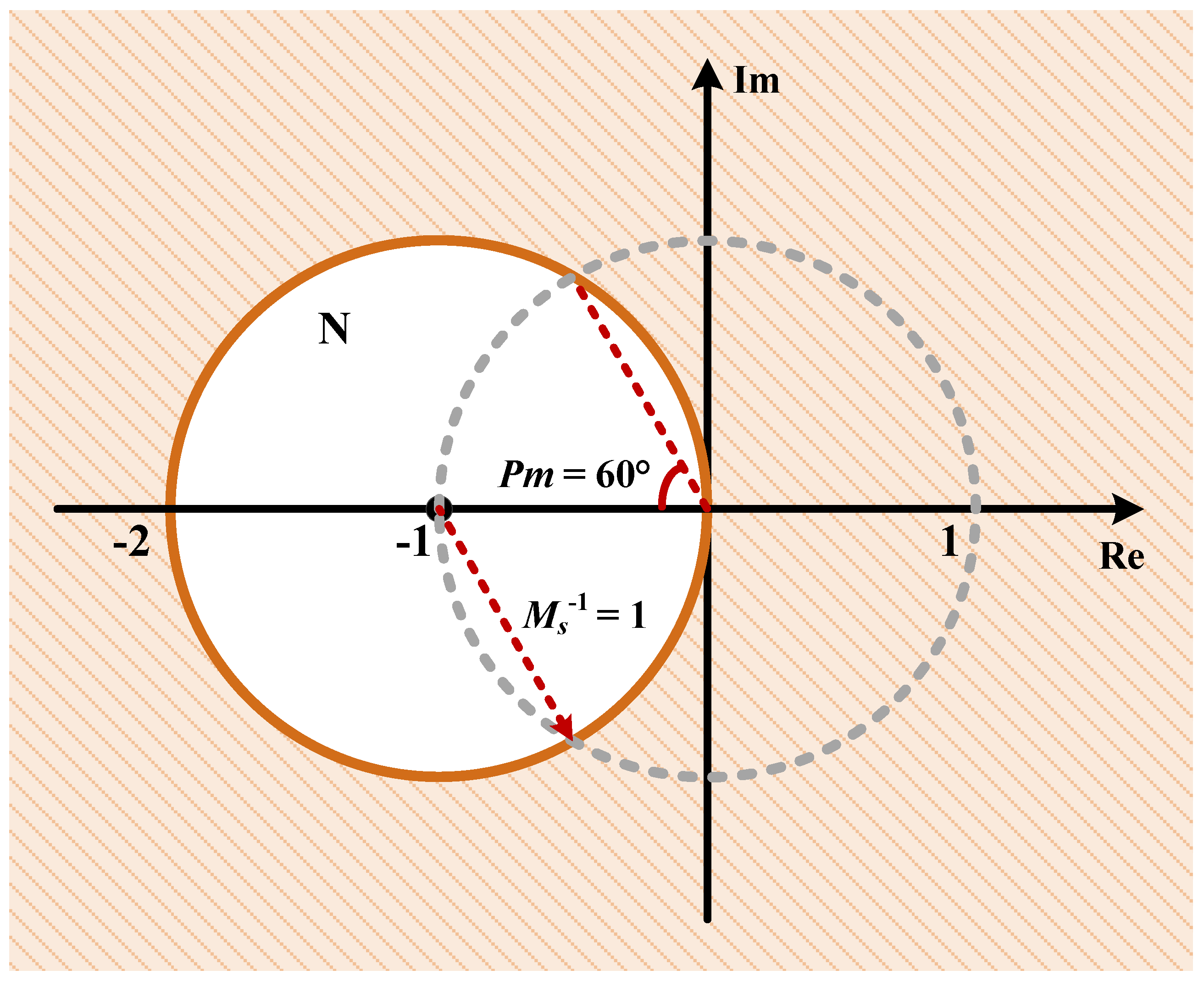
The geometric interpretation of the maximum sensitivity is shown in Figure 5. As can be realized, $M_s$ is an effective way to measure the robustness of the system against modeling uncertainties, in which the lower the value of $M_s$ is, the more robust the system is. Additionally, there is a correlation between $M_s$ and the gain and phase margins, which guarantees the margins given by (23) based on (22) [34].

$$g_m>\frac{M_s}{M_s-1}\to \infty and{p}_m>2arcsin\frac{1}{2M_s}\ge {60}^{\circ }$$

(23)

which means an infinite positive gain margin and 60 degree phase margin. Furthermore, it can be concluded that the Nyquist diagram of $\mathcal{L}\left(j\omega \right)$ will never enter the unit circle N.

As can be understood, the performance and optimality of the control system are contingent to a great extent on the choice of $\mathcal{Q}$ and $\mathcal{R}$ [35]. Generally, they are selected as diagonal matrices such that the quadratic cost function is a weighted integral of the squared error of the states and inputs. Usually, the weighting matrices are adjusted using a trial and error approach, which makes the design procedure a long and laborious task. Hence, this paper utilizes the BA to find the optimal values for the weighting matrices by minimizing an objective function. To this end, there exist multiple performance indices such as integral of absolute error (IAE), the integral of squared error (ISE) or integral of time-weighted-squared-error (ITSE), each of which has its advantages and disadvantages. This paper utilizes the ITSE performance index for tuning the weighting matrices, as given by (24).

$$J={\int }_0^{\infty }t{e}^{2}dt$$

(24)

In this regard, weighting matrices are considered as $\mathcal{R}=r$ and $\mathcal{Q}=diag[q_{11},q_{22},q_{33},q_{44}]$, in which each microbat codes the $q_{ii}$ and r. Furthermore, as shown in Figure 3b, to provide zero steady-state error and regulated output, the LQR control is equipped with a simple integral action leading to the LQI control.

Bat Algorithm

The bat algorithm (BA) is a relatively new meta-heuristic optimization algorithm based on formulating the echolocation behavior of microbats [36]. These bats emit a very loud sound pulse and listen for the echo that bounces back from the surrounding objects. By processing the echoes, they can detect the distance and orientation of the target, the type of prey, and even the moving speed of the prey. Microbats adjust the frequency $f_i\in [f_{min},f_{max}]$, loudness $A_i\in [A_{min},A_{max}]$, and the rate $r_i\in [0,1]$ of their emitted pulses based on the proximity of their target. They increase the frequency of pulses while decreasing their loudness when they fly near their prey until just before contact in which pulses become like a continuous buzz. The constituent steps of BA can be summarized as the schematic pseudo-code shown in Algorithm 1. From the performance comparison of the BA against well-known optimization algorithms like the genetic algorithm (GA) and particle swarm optimization (PSO), it is concluded that the BA is potentially more powerful than the GA and PSO [37].

Algorithm 1: Pseudo code of the bat algorithm (BA)

4. Simulation Results

A three-phase 50-Hz 55-V (line) 5-A Y-connected load with a lagging power factor of 0.8 is fed with an input voltage of 20 V through a ZSI operating at 5 kHz using simple-boost PWM. On the basis of guidelines presented in [38] to design impedance networks, the unknown parameters were selected as listed in

Table 1. Nominal inverter parameters.

Parameter	Symbol	Value
Input voltage (V)	$V_{in}$	20
Capacitor voltage (V)	$V_C$	$89.8146$
Inductor current (A)	$I_L$	$19.05$
Output current (A)	$I_o$	$4.2362$
Capacitor ($\mu$F)	C	$92.25$
Inductor (mH)	L	$2.1$
Load ($\Omega$)	$R_o$	27
Shoot-through duty cycle	D	$0.4374$
Coupling inductor (mH)	$L_o$	$6.6$
Parasitic resistance ($\Omega$)	r	$0.05$
Switching frequency (KHz)	f	10

. It worth noting that the range of the uncertain parameters are $R_o\in [10,60]$ and $D\in [0.3,1]$.

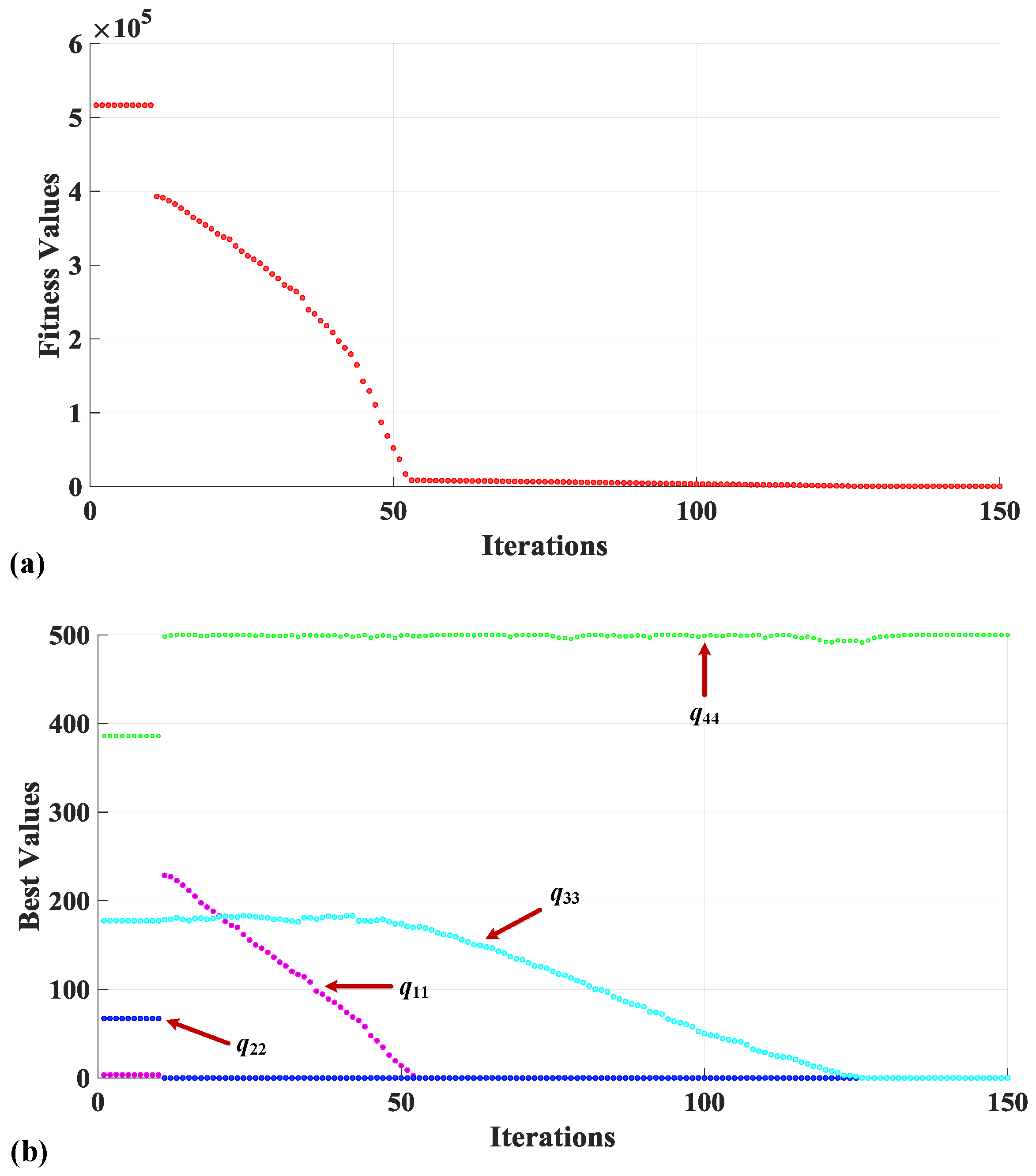
The proposed controller aim and objective is to minimize (18), in which weighting matrices are adjusted by the BA.

Table 2. Bat algorithm (BA) parameters.

Parameter	Value
Loudness	$0.5$
Pulse rate	1
Population size	50
Frequency range	$[0,2]$
Maximum iteration	400
Dimension of search variables	3

provides the required parameters for the successful operation of the BA algorithm. Using (24), the optimization processes are executed and the evolution of the fitness function besides the convergence curves of weighting matrices are illustrated in Figure 6. It can be seen that the tuning parameters quickly converged toward the best solutions after 150 iterations. Accordingly, the global best of the bats, the optimal weighting matrices, are calculated as $\mathcal{R}=1$ and $\mathcal{Q}=diag[0.01,0.01,0.01,500]$. Then, using Matlab to solve (19), the proposed robust LQI controller is computed as (25).

$$K=[0.62410.0153-0.1468-22.3607]$$

(25)

Thus, the corresponding control signal generating the shoot-through duty cycle is calculated as (26).

$$d\left(t\right)=0.6241i_L+0.0153v_C-0.1468i_o-22.3607x_{ext}$$

(26)

To compare the performance and robustness of the proposed controller, the ZSI is also simulated with PI and SF controllers within dual loop schemes presented in Figure 3a,b, respectively. The outer PI controller in Figure 3a is replaced with a simple integral action while the inner PI controller is calculated as (27).

$$\mathrm{PI}=\frac{k_i}{s},k_i=0.0564$$

(27)

To design the SF controller, the well-known Ackermann’s formula given by (28) is adopted.

$$K=[00\cdots 1]{\phi }_C^{-1}\vartheta \left(A_{tot}\right)$$

(28)

where, ${\phi }_C$ is the controllability matrix, and $\vartheta \left(s\right)={(s+w_0)}^{n+1}$ is the desired characteristic equation with order of n. Thus, by setting the desired bandwidth as ${\omega }_0=300$, the SF gain with corresponding control law are derived as (29) and (30), respectively.

$$K=[-0.00070.0031-0.071-0.0211]$$

(29)

$$d\left(t\right)=-0.0007i_L+0.0031v_C-0.071i_o-0.0211x_{ext}$$

(30)

5. Discussion

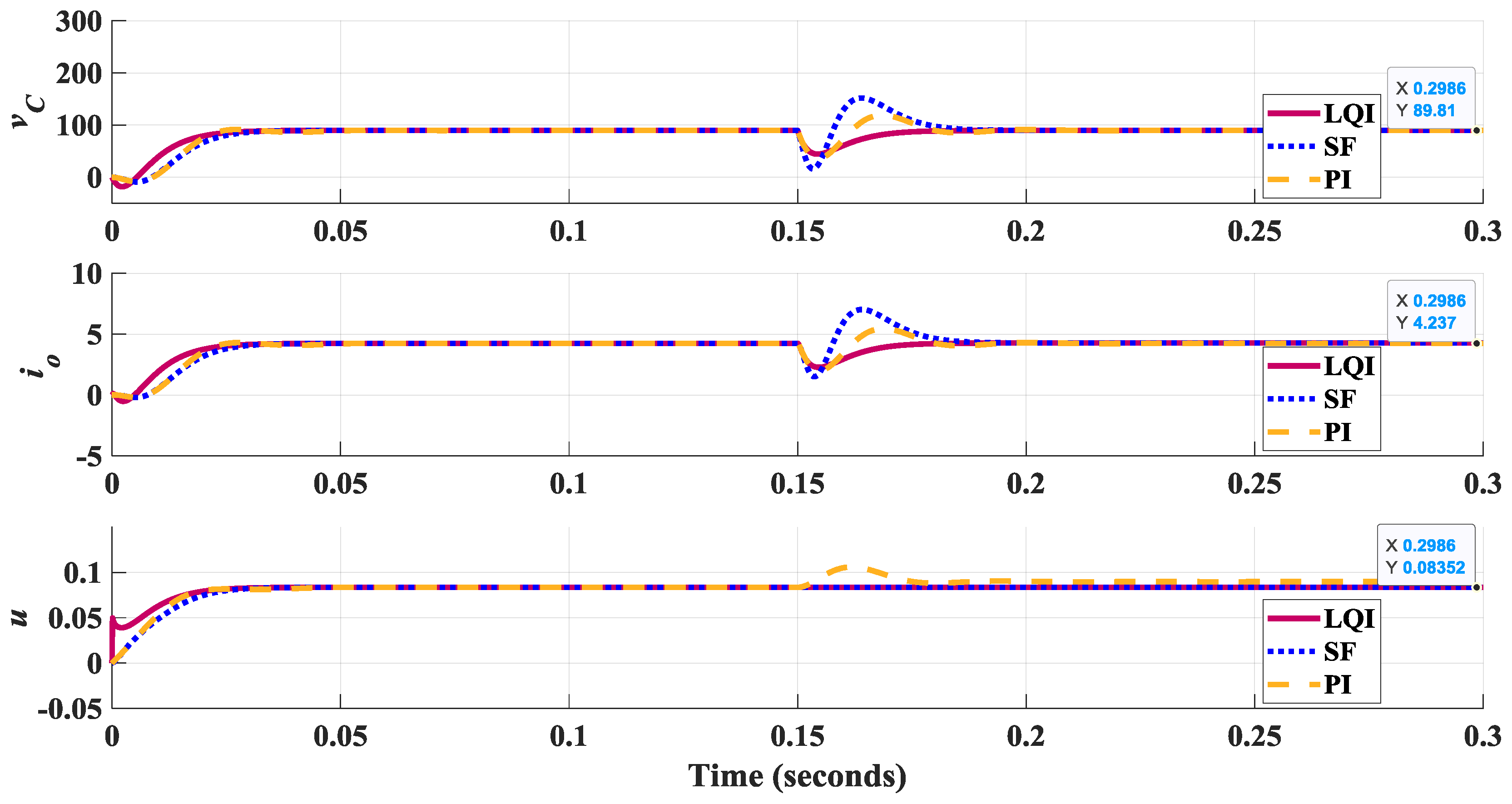
To assess the performance of the presented controller, the closed-loop response of the system is derived in the presence of load disturbance under nominal and perturbed conditions. Figure 7 presents the voltage across the capacitor and output current reaction to a load disturbance 4 A, when the inverter operates at the nominal condition ($D=0.4374$ and $R_o=27$). The corresponding performance indices are summarized in

Table 3. Performance indices of the nominal closed-loop responses ($D=0.4374$ and $R_o=27$).

		Servo Response		Regulatory Response
Controller	TV	IAE	MP(%)	IAE	Peak
PI	0.1285	1.5059	2.21	0.7733	29.1953
SF	0.0835	1.5620	0	1.1866	62.0276
LQI	0.0955	1.3253	0	0.6370	0

for both servo and regulatory problems. It can be recognized that all of the controllers exhibit stable servo and regulatory responses without a steady-state error, due to utilizing an extended integral action. However, the proposed robust LQI controller provides a fast yet no overshoot servo response besides a less undershoot regulatory response. It can be seen that the steady-state voltage across the capacitor is 89.8 V, which has a subtle difference from the designed value of 89.8146, and the output current reached 4.236, which is very close to the designed value of 4.2362. Moreover, the control signals of all comparative methods are smooth enough for the successful operation of the developed ZSI. According to Figure 7, the presented method provides more initial control effort to properly decrease the undershoot value.

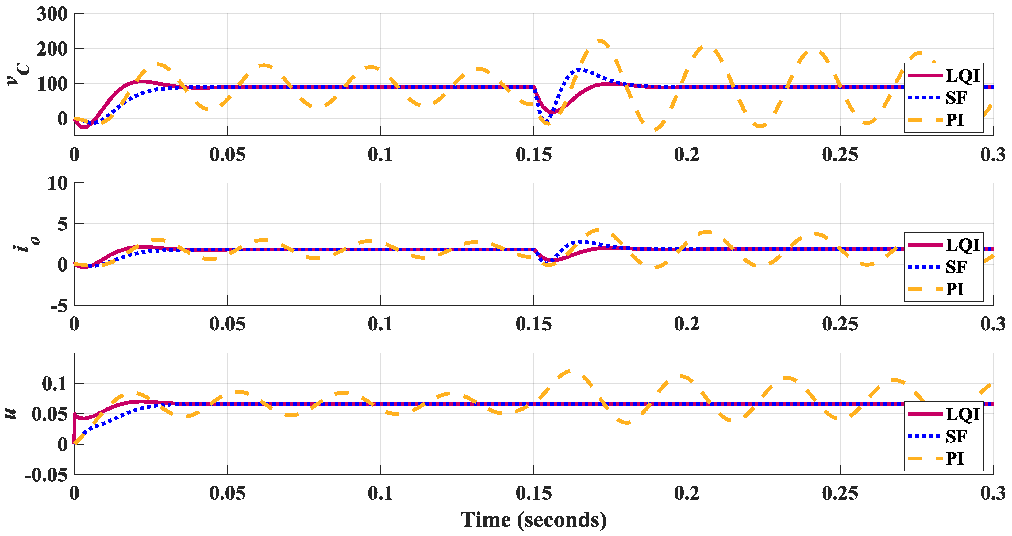
To investigate the robustness to variations in plant parameters, simulations are repeated by keeping the previous parameter setting for the perturbed conditions. Figure 8 presents the voltage across the capacitor and output current reaction to a load disturbance 4 A at the perturbed condition ($D=0.4$ and $R_o=60$).

Table 4. Performance indices of the perturbed closed-loop responses ($D=0.45$ and $R_o=60$).

		Servo Response		Regulatory Response
Controller	TV	IAE	MP(%)	IAE	Peak
PI	0.9684	10.2560	72.3319	8.6512	106.5602
SF	0.0665	1.6569	0	1.1970	48.9907
LQI	0.0922	1.4811	0	0.9914	0

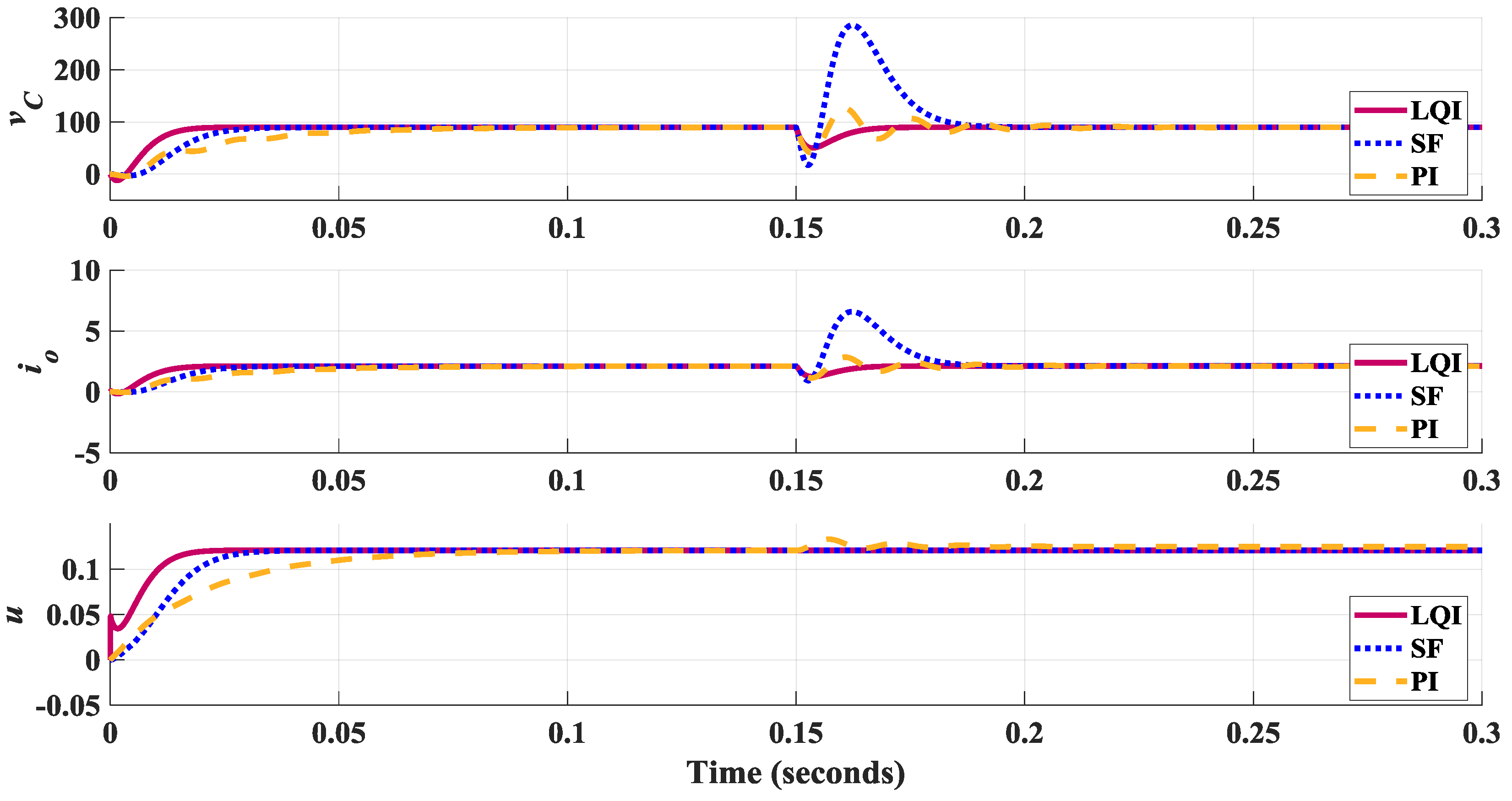
indicates the corresponding performance indices for both servo and regulatory problems. While the SF and LQI-based controllers yield stable performance, the PI-based control system produces a near unstable response. Furthermore, the SF-based control scheme results in unacceptable oscillations in regulatory response, whereas the proposed LQI-based robust controller shows better robustness against the parameter variations by preserving its closed-loop response. To analyze more the robust performance, simulations are repeated at the perturbed condition ($D=0.45$ and $R_o=60$). The corresponding performance indices are provided in

Table 5. Performance indices of the perturbed closed-loop responses ($D=0.4$ and $R_o=60$).

		Servo Response		Regulatory Response
Controller	TV	IAE	MP(%)	IAE	Peak
PI	0.1617	2.1442	0	0.7245	36.8378
SF	0.1209	1.4094	0	2.9993	195.8931
LQI	0.1422	0.9826	0	0.4328	0

for both servo and regulatory problems. As can be understood from Table 5 and Figure 9, PI and SF controllers degraded their transient responses and showed high-frequency small or low-frequency large oscillations in disturbance rejection. The results reveal that despite the perturbed condition, the synthesized controller preserves no overshoot and less undershoot transient responses.

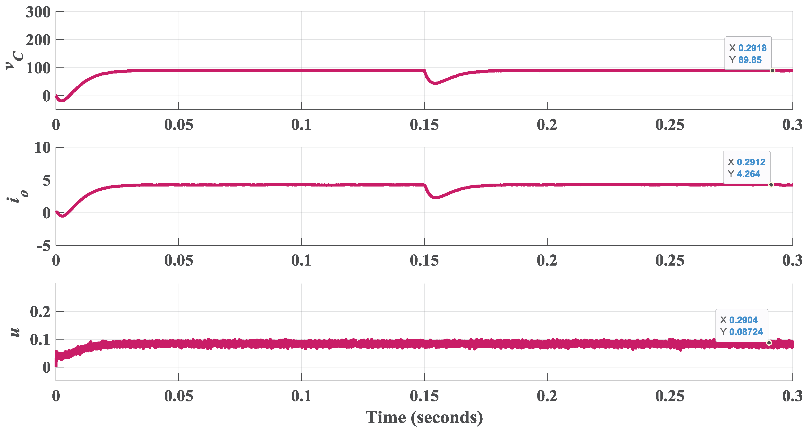
Process noise needs to be included in a model, due to modeling approximations and model integration errors, which shall be investigated when considering closed loop control. For simulations, the process noise is taken into account as Gaussian distribution with zero means and different covariance matrices. The closed-loop response under PI and SF controllers result in unstable responses for a process noise with zero means and covariance matrices of 1. Figure 10 depicts the corresponding voltage across the capacitor and output current signal produced by the proposed controller. It is clear that the proposed controller keeps the performance and robustness of the closed loop system under a process noise with zero means and covariance matrices of 100.

6. Conclusions

This paper addressed the optimal design of a robust LQI controller for a ZSI, considering uncertainties, disturbances, and nonminimum phase issues. The small signal and extended models were explicated using state-space averaging. The ZSI possessed a nonminimum phase characteristic with a real right-half plane zero, which imposed special constraints on the performance of the control system. While load and shoot-through duty-cycle were considered to be uncertain or time-varying parameters with known bounds, external disturbances were modeled as an output current source. The BA optimization algorithm was utilized to find optimal weighting matrices according to the ITSE performance index. The robustness of the proposed method was also investigated using maximum sensitivity criteria. To assess the performance obtained by the proposed controller, the results were compared with PI and SF controllers. Conducted simulation and experimental results demonstrated the efficiency and effectiveness of the proposed robust method in terms of both transient and steady-state.