Article

A 3-D Simulation of a Single-Sided Linear Induction Motor with Transverse and Longitudinal Magnetic Flux

by
Juan Antonio Domínguez Hernández
1,*,
Natividad Duro Carralero
1 and
Elena Gaudioso Vázquez
2
1
Dpto. Informática y Automática, ETSI Informática, Universidad Nacional de Educación a Distancia, Juan del Rosal, 16, 28040 Madrid, Spain
2
Dpto. Inteligencia Artificial, ETSI Informática, Universidad Nacional de Educación a Distancia, Juan del Rosal, 16, 28040 Madrid, Spain
*
Author to whom correspondence should be addressed.
Appl. Sci. 2020, 10(19), 7004; https://doi.org/10.3390/app10197004
Submission received: 16 September 2020 / Revised: 4 October 2020 / Accepted: 5 October 2020 / Published: 8 October 2020
(This article belongs to the Special Issue Modeling, Design and Control of Electric Machines)

Abstract

:
This paper presents a novel and improved configuration of a single-sided linear induction motor. The geometry of the motor has been modified to be able to operate with a mixed magnetic flux configuration and with a new configuration of paths for the eddy currents induced inside the aluminum plate. To this end, two slots of dielectric have been introduced into the aluminum layer of the moving part with a dimension of 1 mm, an iron yoke into the primary part, and lastly, the width of the transversal slots has been optimized. Specifically, in the enhanced motor, there are two magnetic fluxes inside the motor that circulate across two different planes: a longitudinal magnetic flux which goes along the direction of the movement and a transversal magnetic flux which is closed through a perpendicular plane with respect to that direction. With this new configuration, the motor achieves a great increment of the thrust force without increasing the electrical supply. In addition, the proposed model creates a new spatial configuration of the eddy currents and an improvement of the main magnetic circuit. These novelties are relevant because they represent a great improvement in the efficiency of the linear induction motor for low velocities at a very low cost. All simulations have been made with the finite elements method—3D, both in standstill conditions and in motion in order to obtain the characteristic curves of the main forces developed by the linear induction motor.

1. Introduction

A linear induction motor (LIM) is a type of asynchronous machine that in comparison with the traditionally rotary induction machine does not develop an electromagnetic torque [1]. The electromagnetic forces in an LIM operate along two directions: horizontal and vertical, instead of rotating. Figure 1 illustrates the process for generating the electromagnetic forces in an LIM [2].
As shown in Figure 1, a, LIM has two different parts, which produce two different magnetic fields. The first part is a ferromagnetic steel (called stator or primary part). Inside this part, is located an alternating current (AC) three-phase winding that generates a traveling magnetic field. The second part is composed of two joined layers of aluminum and iron (called rotor or secondary part), where the generated eddy currents produce a new magnetic field. The interaction between the two magnetic fields created in both parts causes the motion of the secondary part.
The relevance of LIMs in the industry is huge because there are a lot of applications in different areas [3], such as transportation systems (propulsion of wheel-on-rail vehicles and magnetic levitation high-speed trains), vertical drives (passenger elevator or an elevator without ropes), industrial drives (impact machine and machine tools), or automotive control and robotic. Additionally, these motors are relevant in military applications [4], such as electromagnetic aircraft launch or electromagnetic rail gun systems. Besides, LIMs are very important in all magneto-hydrodynamic applications because under low-velocity conditions, an LIM can be used as an electromagnetic pump where the liquid metal represents the moving part.
A general classification of LIMs [1], divides these electrical induction machines into two different families depending on two criteria: the configuration of the magnetic flux and the geometry of the machine. The first family can be divided into two categories depending on the number of primary parts. Hence, an LIM that operates with only a primary part is called single-sided linear induction motor (SSLIM) and an LIM with two primary parts is called double-sided linear induction motor (DSLIM). The second family can be also divided into two different categories. First, an LIM with a magnetic flux that circulates along the direction of the movement called a longitudinal flux linear induction motor (LFLIM). Second, an LIM with a magnetic flux closed to a perpendicular plane to the direction of the movement called a transverse flux linear induction motor (TFLIM) [5,6].
The most popular topology in the literature is LFLIM. However, TFLIM presents some advantages [1], such as a magnetic flux that crosses the airgap twice, a reduction of the consumed magnetization current, and a reduction in the weight of the device. In the literature, there are several techniques to increase the efficiency of LIM´s which can be classified into the three following strategies. The first strategy is called winding skew and it is oriented to reduce the ripple whose effects are unwished [7]. The second strategy is focused on employing the third-order harmonics current injection to improve the thrust and the levitation force [8] and the third strategy modifies the geometric parameters of the LIM [9,10,11,12,13].
Our paper is focused on the third strategy that allows us to modify the magnetic flux configuration inside the armature on the LIM and redesign the paths available for the eddy currents induced inside the aluminum plate. The starting point is a prototype of an LIM that will be called model 1. Model 1 is an SSLIM with a configuration of TFLIM, whose geometry has been modified in both parts (primary and secondary part) in order to improve the efficiency of the LIM. Changes in the geometry have been introduced to configure a relevant three dimensions main magnetic circuit (3D-MMC). Our goal is to search two useful paths in perpendicular planes available for the magnetic fluxes. This novel configuration will be called mixed flux magnetic linear induction motor or hybrid flux magnetic linear induction motor (MFLIM) where longitudinal and transverse fluxes are operating simultaneously.
The objective of the paper will be carried out using three different models that will be explained in the following sections. In model 2, the aluminum layer geometry will be modified. Next, in model 3, the back iron belonging to the primary part will be redesign as well. The last model, model 4, will present a geometry capable to generate a high thrust force without increasing the fixed electric supply used in model 1, due to an increment of the width of the transversal slots in the primary part. All models are simulated with the three-dimensional finite elements method (FEM-3D) used to design electromagnetic devices [14,15].
This paper is organized as follows. Section 2 describes the original model (model 1), its geometry, its electric and magnetic properties, and the simulation conditions using FEM-3D. In Section 3, model 2, model 3, and model 4 are explained. Section 4 details the simulation results for each model in standstill conditions and also take into account the motion in the TFLIM. Finally, the main conclusions obtained are presented in Section 5.

2. Original Developed Model

In this section, the original model is described, called model 1. Its technical features (electric and magnetic coefficients, parameters of the primary winding, and dimensions) and the principal reasons for its construction are detailed. In Section 3, all modifications made to its geometry will be justified.
Model 1 was built in the 90s by the Spanish Polytechnic University in Madrid [16]. The objective was the definition of a new formulation that could explain the exact behavior of a TFLIM. This model included the improvements between the theoretical and experimental results obtained in the laboratory. All experimental tests made in [16] were done with the moving part blocked, therefore its velocity was considered equal to 0 m/s. The two main conclusions of these experiments were the following: first, it was necessary to modify the geometry of the motor to generate a longitudinal magnetic flux into the TFLIM and to minimize the anti-thrust force generated by the lateral teeth. Second, the analysis of the model was simulated with FEM-3D, in order to consider the longitudinal and transversal end effects into the characteristic forces of the LIM.
The main features of the motor are described in the following subsections. Section 2.1 details the geometric parameters of the TFLIM. Section 2.2 shows a graphical representation of the primary winding. Section 2.3 explains the justification of the electric and magnetic properties of the materials and the type of B-H curve assigned to the ferromagnetic regions of the LIM that used in FEM-3D.

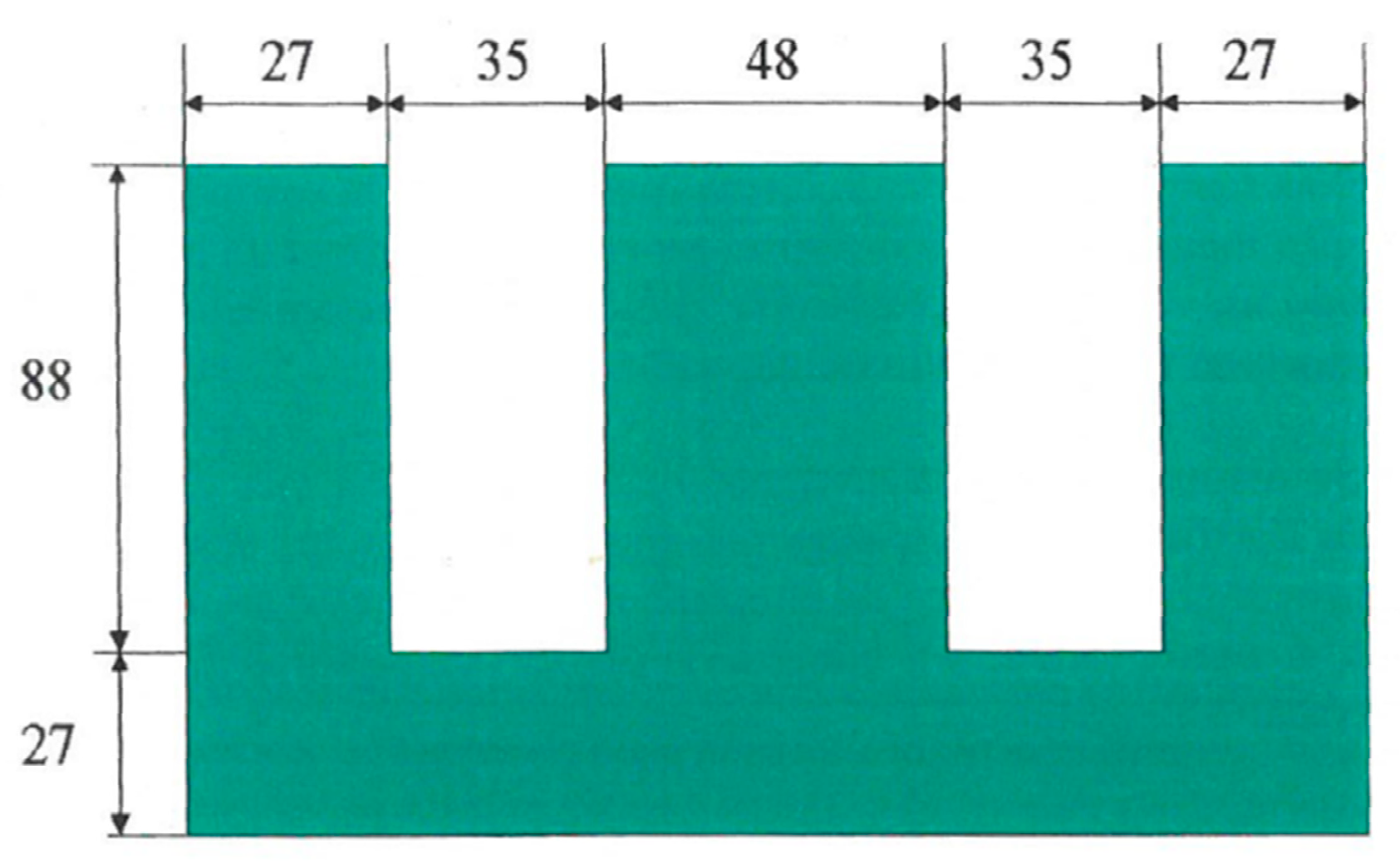
2.1. Geometric Parameters

The modeled TFLIM was composed of a primary part built with 31 magnetic sheets with an E-shaped design [5]. In the moving part, there were two available layers. The first layer was an aluminum plate and the second layer was made of ferromagnetic material, located over the first. Table 1 shows the principal geometric parameters of the TFLIM. Figure 2 shows a transversal view of one ferromagnetic sheet that includes its principal dimensions. More details can be found in reference [16].

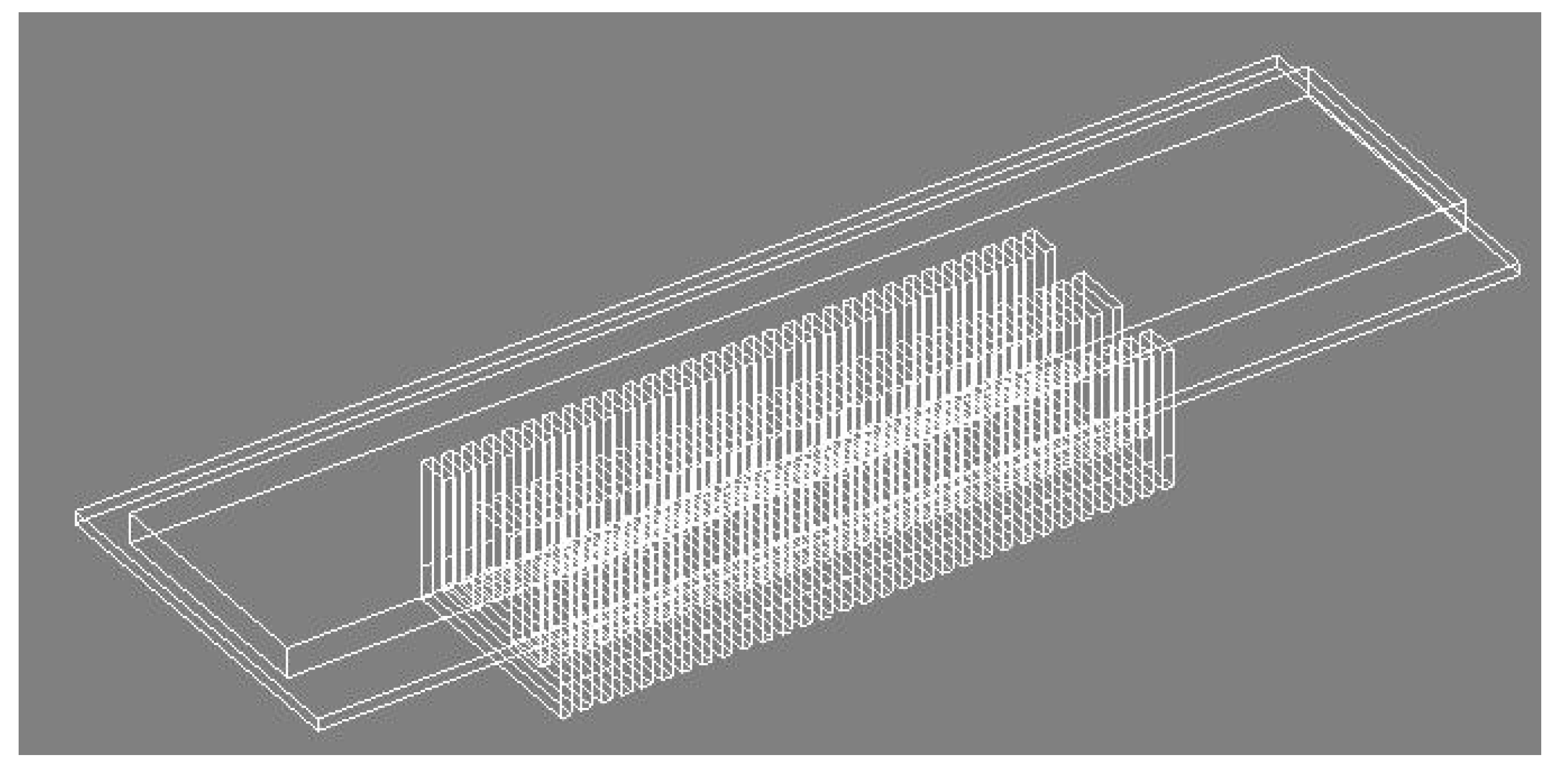
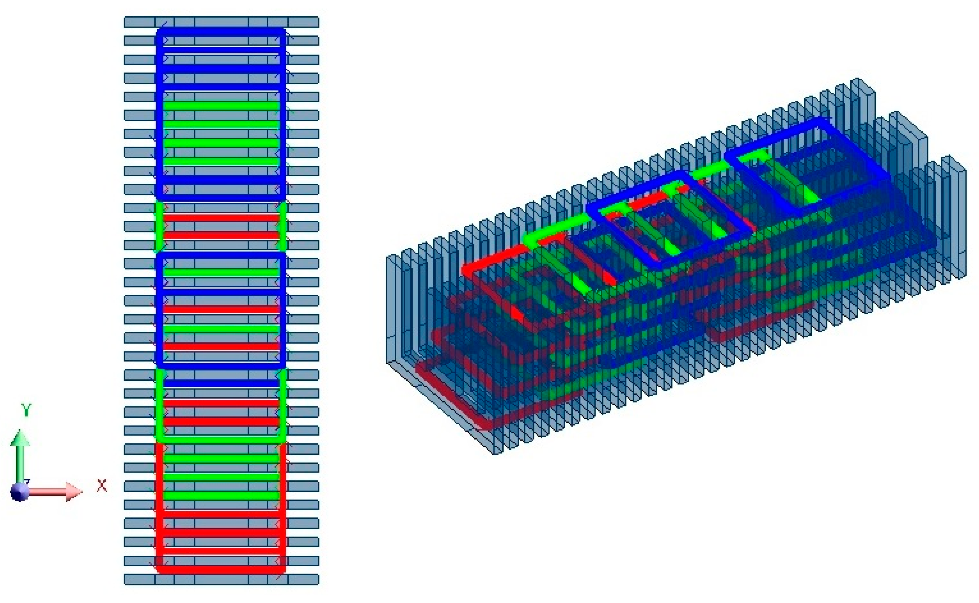
2.2. Graphical View of the Winding in the Primary Part

Figure 3 shows a 3-D view of the different parts of the model 1. The length of the primary part, where the winding is located, is shorter than the secondary or moving part. The dynamic end-effects of this configuration would be different if the dimensions of the aluminum and the back iron in the secondary part were shorter than in the primary part.
The primary AC three-phase winding built with FEM-3D is represented in Figure 4. It shows the distribution of each phase inside the primary core. The red coils at the beginning of the winding belong to phase A. The green coils correspond to phase C and the blue coils located at the end represent phase B. Under these conditions, a traveling magnetic field is developed by the primary winding.
Thus, the primary winding is characterized by two parameters: q that indicates the number of slots per pole and phase (q is equal to 4) and the pole pitch, τp, that corresponds to a value of 200 mm [16]. The traveling magnetic field is defined by a linear velocity called synchronous velocity, v S y n c h r o n o u s (expressed in m/s) according to Equation (1). This velocity depends on the pole pitch and on the frequency linked to the AC three-phase system. In this paper, the LIM is supplied by a fixed frequency equal to 50 Hz, which could be selected by a converter and in consequence, the synchronous velocity will be variable [17].
v Synchronous = 2 · τ p · f = 20   m / s
Once the traveling magnetic field is generated, the thrust and levitation forces are developed by the moving part of the LIM. This secondary part is characterized by a linear velocity, v m o v i n g _ p a r t , different from the v S y n c h r o n o u s . Both velocities depend on a parameter called slip, s, defined by Equation (2), and explained in [17]. In our work, initially, the moving part was blocked. So, the velocity of the moving part was equal to 0 m/s, and the slip equal to one. Under these dynamic conditions, thrust force was into the motor zone, and the levitation force belongs to the repulsive zone. Figure 5 represents the operation point selected for the LIM in this situation. Once standstill condition can be studied widely, the TFLIM can also be simulated, taking into account all slips in the range from 1 to 0.
s = v S y n c r o n o u s v m o v i n g _ p a r t v S y n c r o n o u s v m o v i n g _ p a r t = 0   m / s = 1

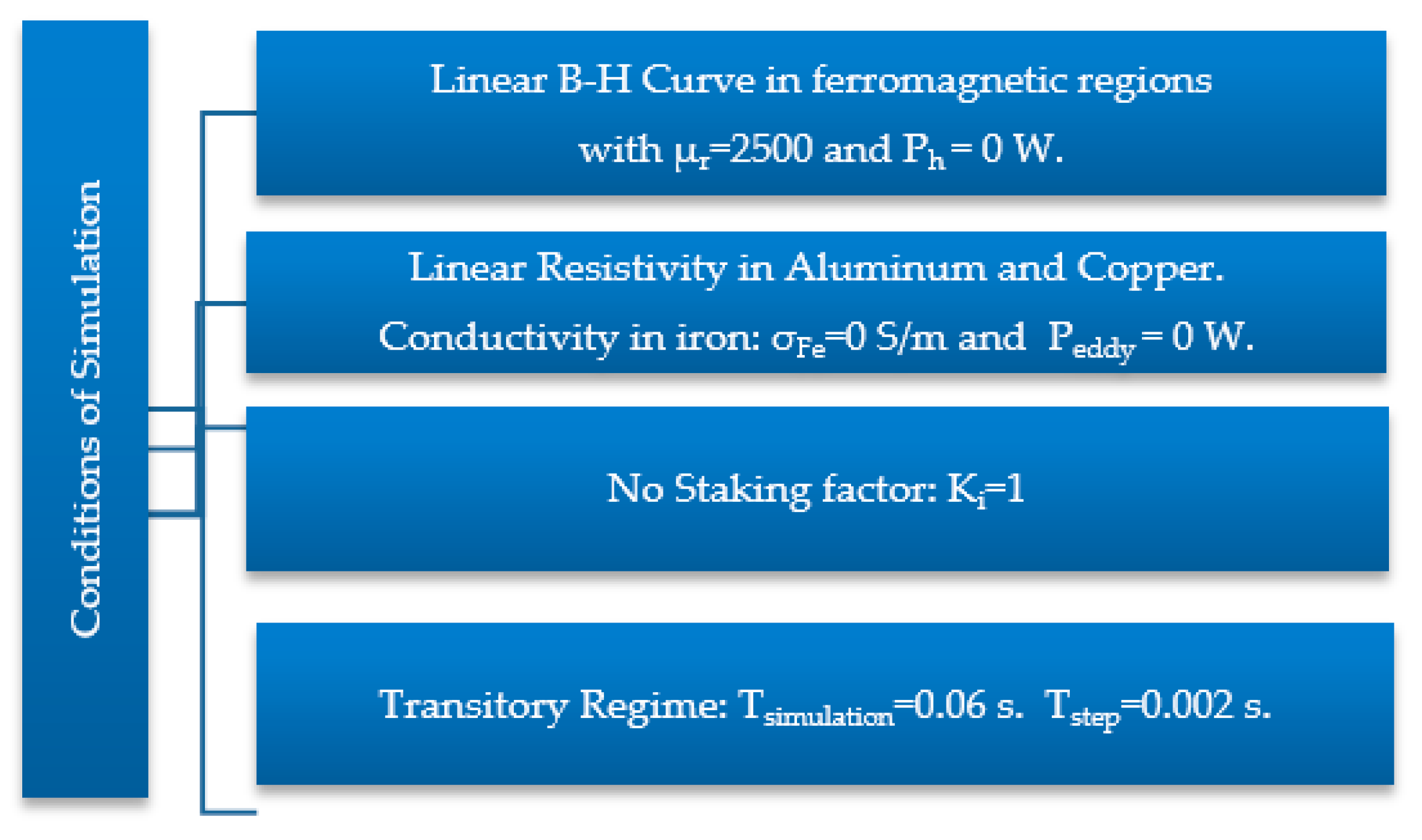
2.3. Electric and Magnetic Properties of the Materials Used in FEM-3D

To simulate the models with FEM-3D, we considered two electrical and magnetic properties: electrical resistivity and magnetic permeability. Table 2 shows the values selected for the simulations. The electrical resistivity of the materials in the moving part is given by its inverse value, the electric conductivity.
With respect to the magnetic permeability (B-H curve), soft ferromagnetic materials were used for the laminated cores of electrical machines. The shape of the B-H curve was simplified to a straight line with a constant slope given by the relative permeability, µr, according to Equation (3), as explained in [18]:
μ r d = μ r = d B μ 0 · d H = c t e B = μ 0 · μ r · H
where μ r d is the differential relative permeability; μ 0 : 4 · π · 10 7 H m is the magnetic permeability of free space; B is the magnetic field density vector (T); H is the magnetic field intensity (A/m).
With these parameters, the behavior of the motor had two relevant consequences: the zero electric conductivity of the steel implied the absence of eddy currents in the ferromagnetic parts (second layer in the moving part and primary part) and the linear B-H curve implied that there are not regions inside of the LIM working under magnetic saturation conditions. For these reasons, the iron losses are neglected in the simulations with FEM-3D, according to Equation (4). See references [19,20].
P F e = P e d d y σ F e = 0 S m = 0   W . + P h L i n e a r   B H   C u r v e = 0   W = 0   W .
where P F e is the power losses in core iron (W); P e d d y is the power eddy currents losses (W); P h is the power hysteresis losses (W). A practical recommendation to reduce eddy currents losses is to build the ferromagnetic cores by coated double-sided areas with a thin layer of insulation, usually oxide insulation. To quantify this, the stacking factor K i was used as a ratio defined by Equation (5), as explained in [21].
K i = d l d l + 2 · Δ i Δ i = 0   m m . = 1
where d l is the thickness of the bare sheet (mm); Δ i is the thickness of one-sided insulation (mm). Nevertheless, to reduce the computing time and the number of nodes in the domain of the FEM-3D, theses insulated areas were not considered (i.e., Δ i = 0 mm). All ferromagnetic regions in our work used a value of stacking factor equal to one; K i = 1.

3. Modified LIM Models and Implementation with FEM-3D

In this section, we describe the modifications made in model 1 to obtain model 2, model 3, and model 4. In addition, we describe the main issues that we have to take into account to simulate them with FEM-3D. The TFLIM prototype (model 1), described in Section 2, will be modified to improve the thrust force. To this end, three different new models were developed:
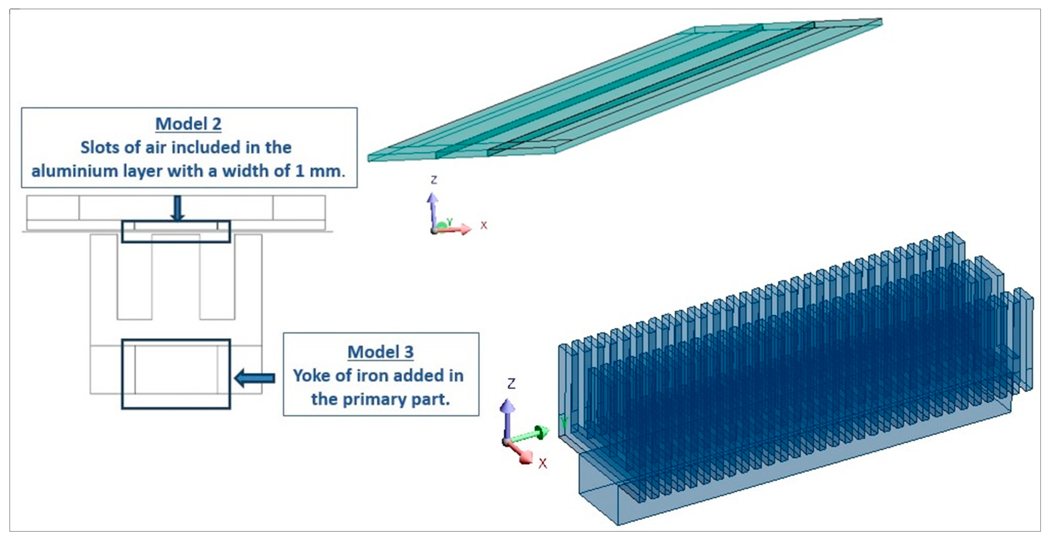
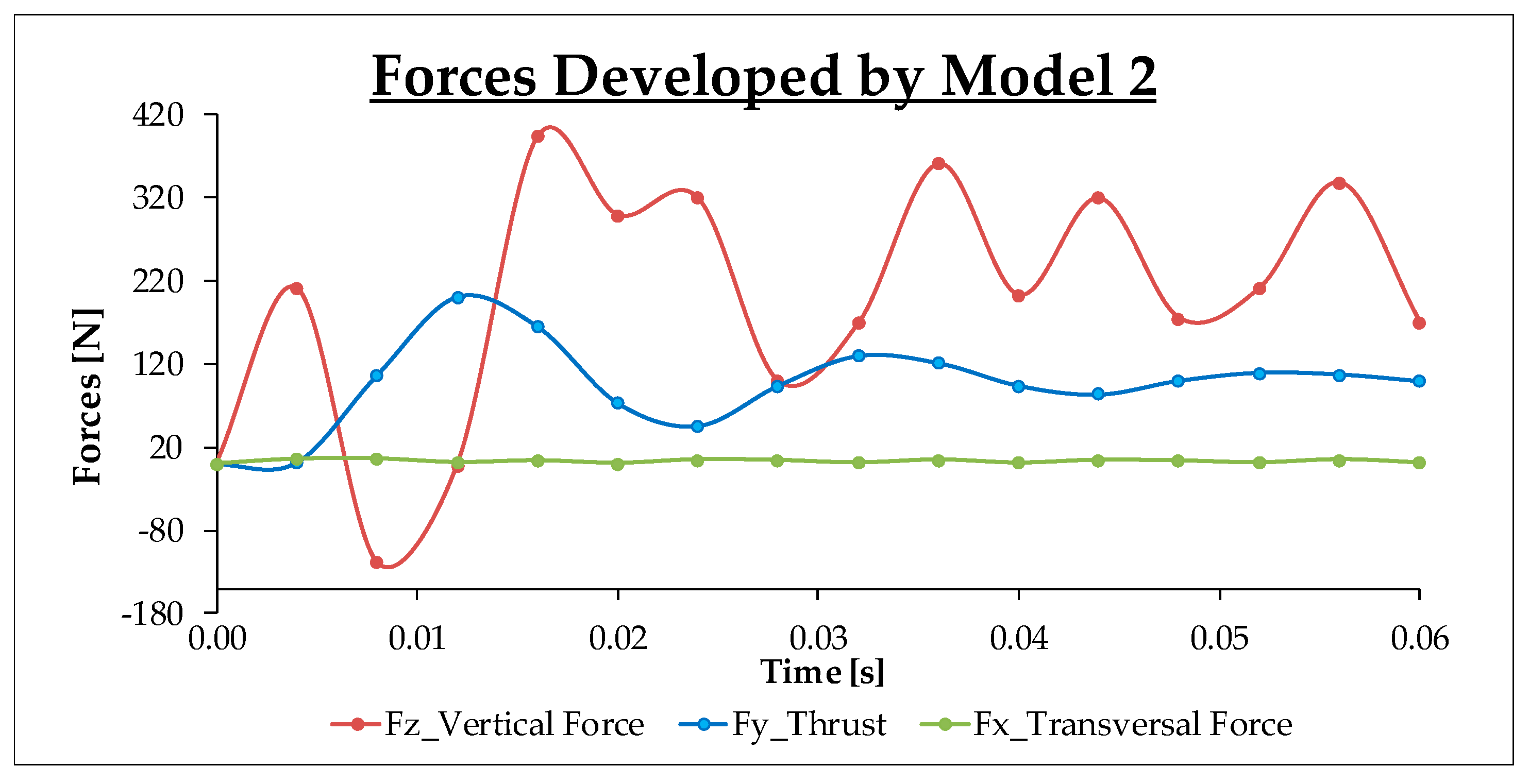
  • Model 2, where the moving part was redesigned. More concretely, the aluminum layer was modified with the introduction of two narrow slots of air or diamagnetic material (µr = 1). Each slot has a width of 1 mm and they are located symmetrically at 108 mm from the edge of the aluminum layer (see Figure 6). The new regions, insulated electrically, allowed us to have three regions available inside the aluminum layer with new paths for the eddy currents, so that each zone of aluminum was located above lateral and central teeth. Consequently, the thrust force originated over the lateral teeth developed along the direction of the motion.
  • Model 3, where the primary part included a ferromagnetic yoke located under the central teeth. The high of this ferromagnetic block was 50 mm, its width was 83 mm, and it was extended along 503.5 mm that corresponded with the length of the LIM. With this new block, the motor produced a longitudinal flux that operated through the main magnetic circuit with the transversal flux. So, the combined action of these fluxes provided a higher thrust force. Figure 6 shows the changes included in model 2 and model 3.
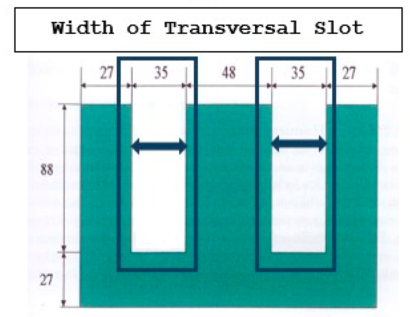
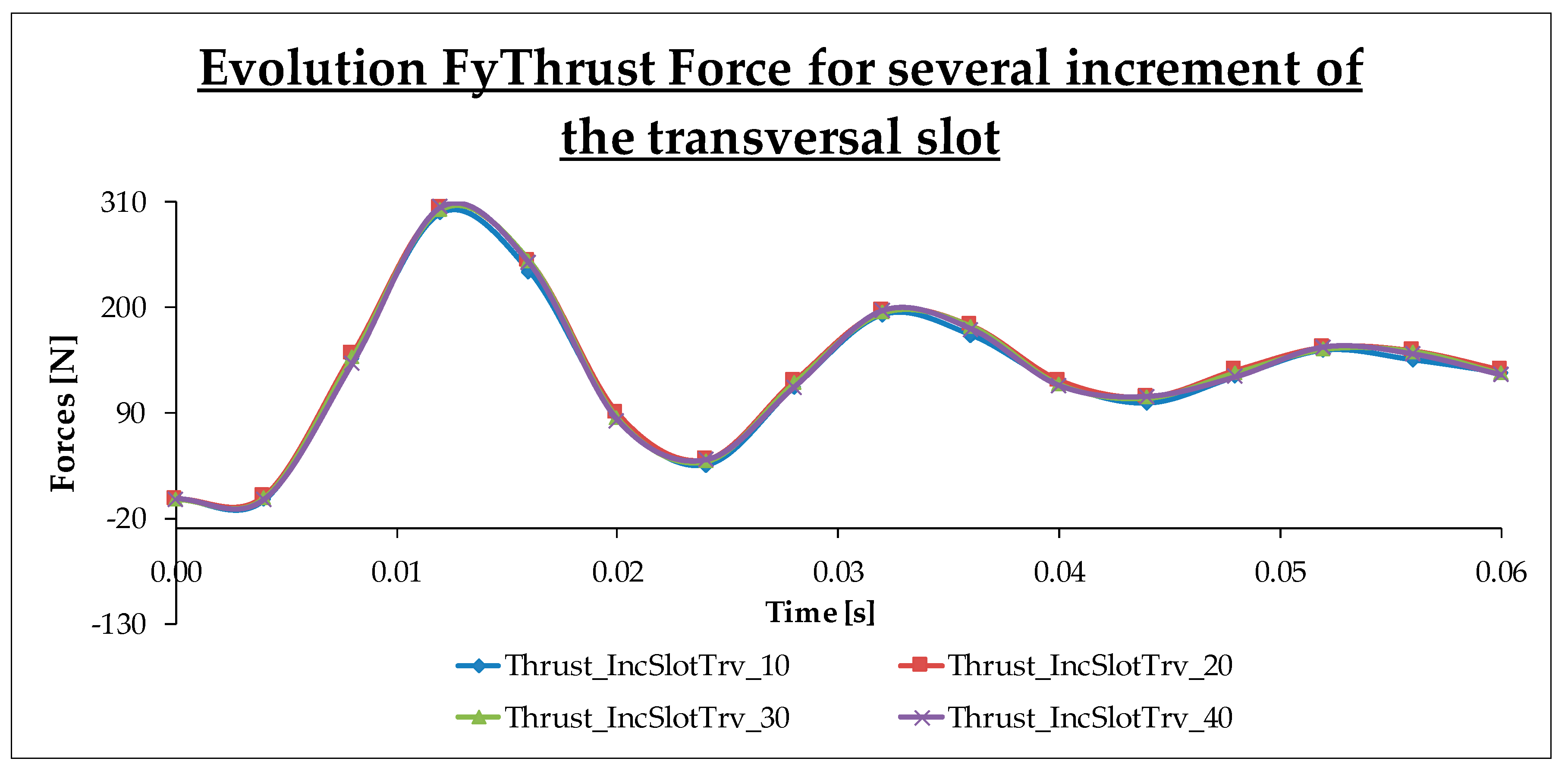
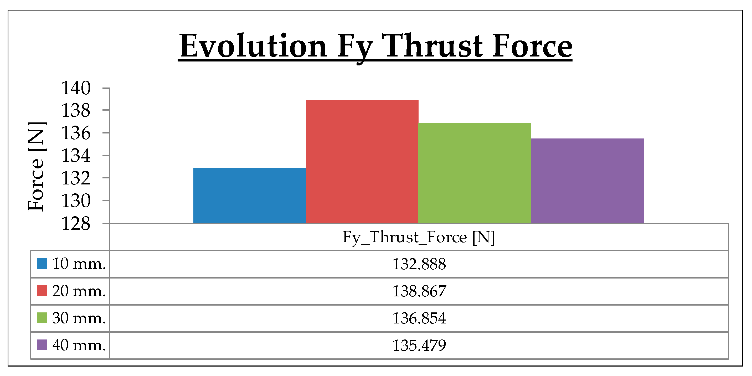
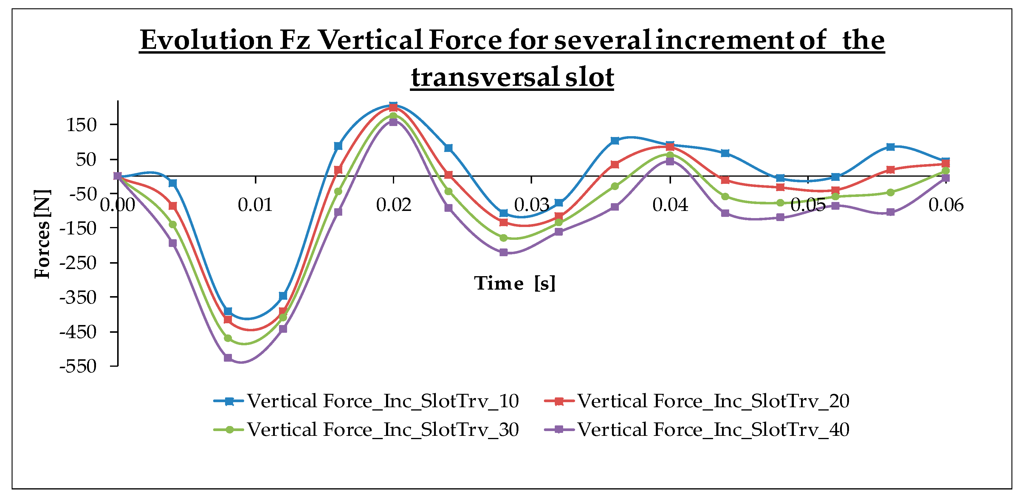
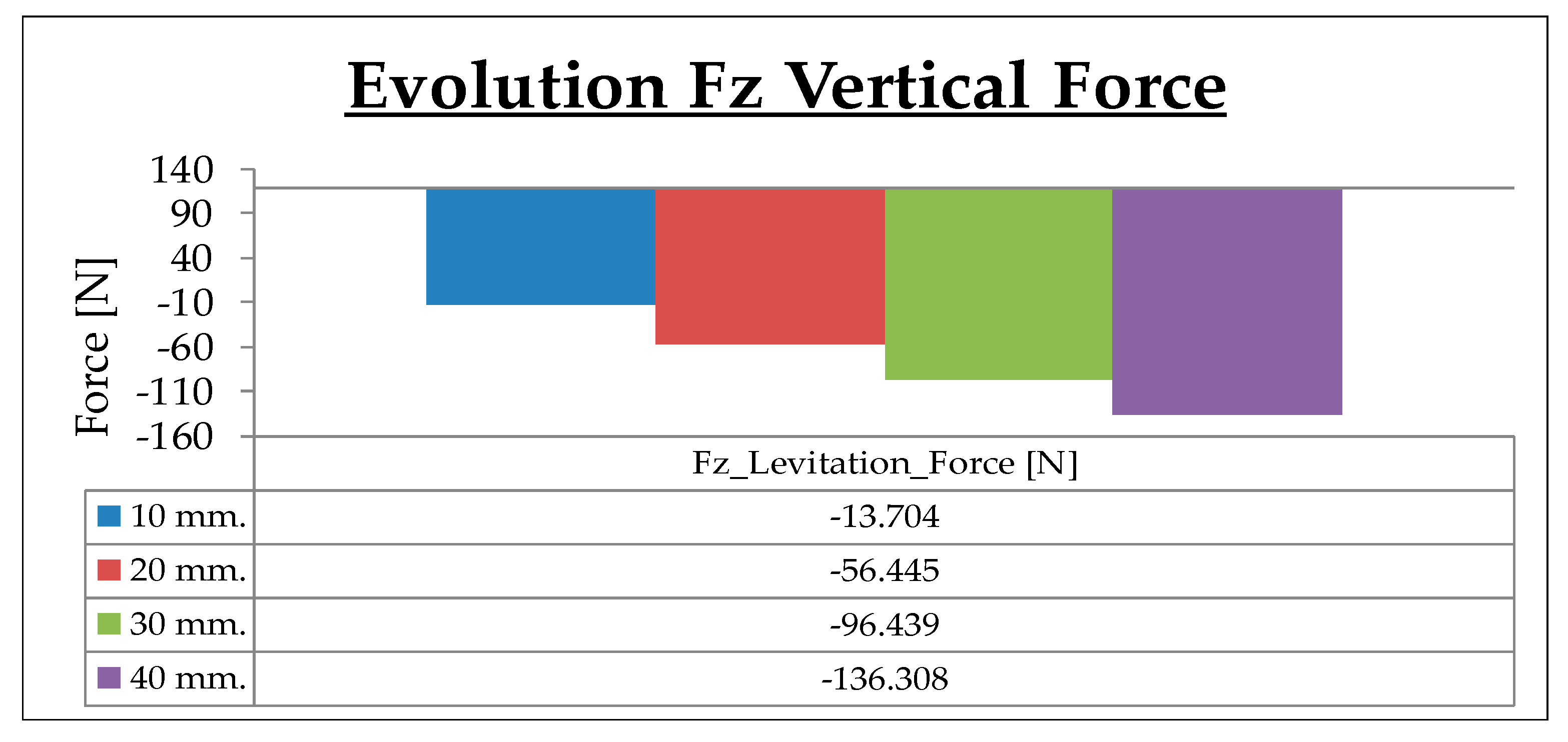
  • Model 4, where the initial dimension of the width of the transversal slots in the primary part (35 mm) was incremented along the direction of the x-axis (see Figure 7) in order to reach a maximum thrust force. The width of the transversal slots was increased from 10 to 40 mm. This model incorporated all the changes proposed in the previous models. It was important to comment that the width of the lateral teeth was not going to be modified although the dimension of the transversal slots was increased along the x-axis. During this study to optimize the thrust force the width of the lateral teeth was fixed to 27 mm.
For the implementation of the models with FEM-3D, the time domain selected corresponds to a transitory state. In all simulations, the frequency f is fixed at 50 Hz. The computation process time was calculated using three types of times: T c y c l e (called cycled time) is the period of the AC voltage signal employed during the simulations [s]; T s i m u l a t i o n (s) (called simulation time), is the number of cycles necessary to achieve the stationary state which allows us to evaluate the advantages of the proposed changes without increasing the computation effort; T s t e p (called step time simulation) is the fraction of the T c y c l e necessary to converge to the solution (s). The T s i m u l a t i o n is defined as three times the T c y c l e , which is divided into 10 steps to fix T s t e p (see Equation (6)). These times were selected experimentally, after several simulations that achieved the correct model.
T c y c l e = 1 f = 0.02   s . { T s i m u l a t i o n = 3 · T c y c l e = 0.06   s . T s t e p = T c y c l e 10 = 0.002   s .
Finally, Figure 8 resumes all necessary conditions to simulate correctly all models proposed:

4. Model Simulations with FEM-3D

This section describes the simulations of all models with FEM-3D. All simulations were carried out with Altair Flux 3D, a finite element software focused on electromagnetic, electric, and thermal design of electric machines. It allowed for optimization of the performance of the machine, efficiency, dimensions, and weight. Section 4.1 establishes the steps to define the electrical supply of the LIM. Section 4.2 presents an analysis of the magnetic field density along the airgap. Section 4.3 shows the simulation results for the different models in standstill conditions and finally, Section 4.4 includes the simulation results with motion.

4.1. Definition of the Electrical External Circuit Coupling

To start the simulation with FEM-3D, the electrical circuit coupling necessary to operate with the LIM was set up. To this end, the following steps were necessary:
  • Step 1: To fix the magnetic field density in the airgap, Bg, using an analytical method to estimate its value [22].
  • Step 2: To select the configuration of the electrical circuit coupling to supply the device (Y-connected or D-connected system) and to generate the traveling magnetic field defined in Section 2.2.
  • Step 3: To use an iterative simulation process to calculate the parameters necessary to define the electrical circuit coupling. The first parameter is the value of the symmetrical line voltage, VLINE. The other parameters are the number of turns per phase and its resistance value: Nphase and Rphase. Both are necessary to have the coils defined correctly. The initial value of Rphase is fixed at around 2.6 Ω to start the iterative process.
In the first step, the magnetic field density in the airgap was considered equal to the average value obtained from Equations (7) and (8), (see reference [22]). Both equations allowed for the obtaining of the value of the first harmonic of Bg, called Bg1, considering only the geometric parameters of the LIM and not their electrical quantities. So, there were two possibilities to calculate Bg1, using Equations (7) or (8).
B g 1 _ I = 0.464 · τ p 1 6
B g 1 _ I I = B t s k i s · ( 1 b o s τ s )   B t s = 5.47 · f 0.32 B g 1 = 5.47 · f 0.32 k i s · ( 1 b o s τ s )
where Bts is the flux density in the primary tooth (T); k i s is the primary stacking factor equal to 1; b o s is the primary slot opening equal to 8.5 mm; τ s is the slot pitch equal to 16.5 mm; τ P is the pole pitch equal to 200 mm, and f is the frequency equal to 50 Hz. At the end, the value of B g 1 is given by Equation (9) and is equal to 0.761 T.
B g 1 = B g 1 _ I + B g 1 _ I I 2 = 5.47 · f 0.32 k i s · ( 1 b o s τ s ) + 0.464 · τ p 1 6 2
In the second step, the coils from the primary winding were supplied by a Y-connected three-phase voltage. This situation is described by the Equation system (10), (11), and (12) (see reference [21]), which generates a traveling magnetic field along the desired direction.
V P h a s e _ a = V L I N E · 2 3 · cos ( ω · t ) = V L I N E · 2 3 · cos ( 2 · π · f · t )
V P h a s e _ b = V L I N E · 2 3 · cos ( ω · t 2 · π 3 ) = V L I N E · 2 3 · cos ( 2 · π · f · t 2 · π 3 )
V P h a s e _ c = V L I N E · 2 3 · cos ( ω · t + 2 · π 3 ) = V L I N E · 2 3 · cos ( 2 · π · f · t + 2 · π 3 )
where VLINE is the voltage established in a Y-connected symmetrical three-phase system (V); V P h a s e _ a , V P h a s e _ b ,   V P h a s e _ c are the supply voltages per phase (V); ω is the angular frequency (rad/s) and t is the instantaneous time of simulation (s).
In the third step, VLINE and Nphase were calculated by the simulations. When the value of Bg reached the value of the magnetic field density established in the first step, VLINE and Nphase were fixed. The measure of Bg was determined with a plane that crosses the mechanical airgap by its middle section (a detailed study of Bg is made in Section 4.2). The results obtained were the following:
V L I N E [ V ] = 660       N p h a s e [ t u r n s c o i l · p h a s e ] = 22
Once Nphase was known, it was possible to calculate the equivalent resistance of the winding linked to a one-phase according to the Equation (14):
R P h a s e [ Ω ] = ( N p h a s e · ρ C u · L ¯ C o i l S w i r e _ C u ) · n P h a s e = 1.29   Ω
where L ¯ C o i l is the average length of a single coil equal to 526.5 mm; Swire_Cu is the section of the copper conductor equal to 1.7 mm2; ρ C u is the resistivity assigned to the copper wire equal to 2.37 ×   10 2 ( Ω · mm 2 / m ) (see Table 2), and nphase is the number of coils per phase equal to 8.

4.2. Analysis of the Magnetic Field Density in the Airgap

To analyze the magnetic field density in the airgap, we represent in Figure 9 its spatial evolution (third component) along the airgap, Bgz with FEM-3D. The distribution of Bgz was calculated over the central teeth and the lateral teeth, with three paths located exactly in the middle plane of the airgap. The blue line corresponds to the component z of the magnetic field density when it crosses the airgap over the central teeth. The other two lines (yellow and green), that are superimposed, belong to the third component of the magnetic field density when it crosses the lateral teeth. For all lengths of the airgap, measured in m in Figure 9, the value of Bgz over the lateral teeth was approximately half with respect to the value of Bgz over the central teeth and it was in the opposite direction (Figure 9).
A similar result was obtained in [16] that included the measurements in the laboratory of the magnetic field density at the top of the lateral and central teeth using explorer coils located around each tooth. We have used these results from [16] to check the validity of our method.
Consider the following points to design the magnetic field density along the airgap:
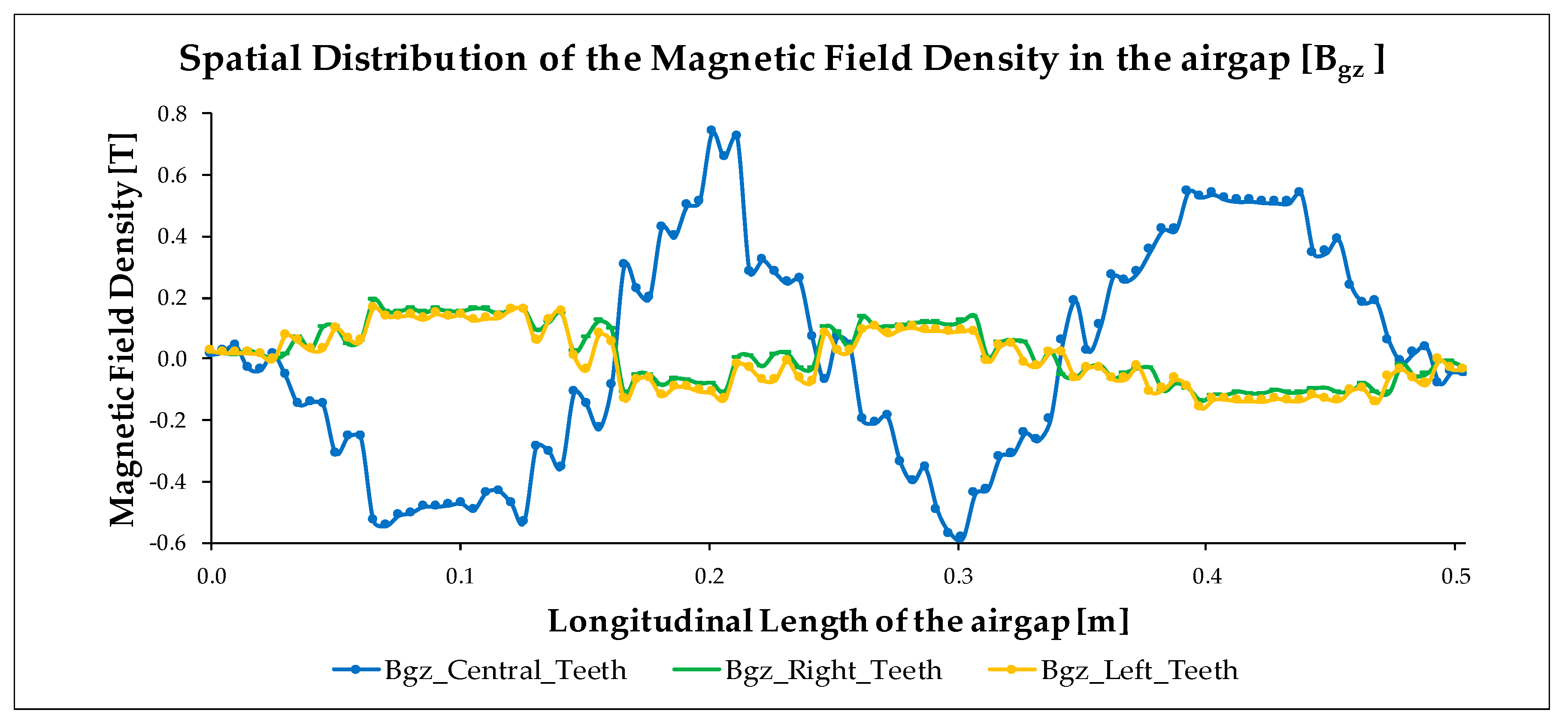
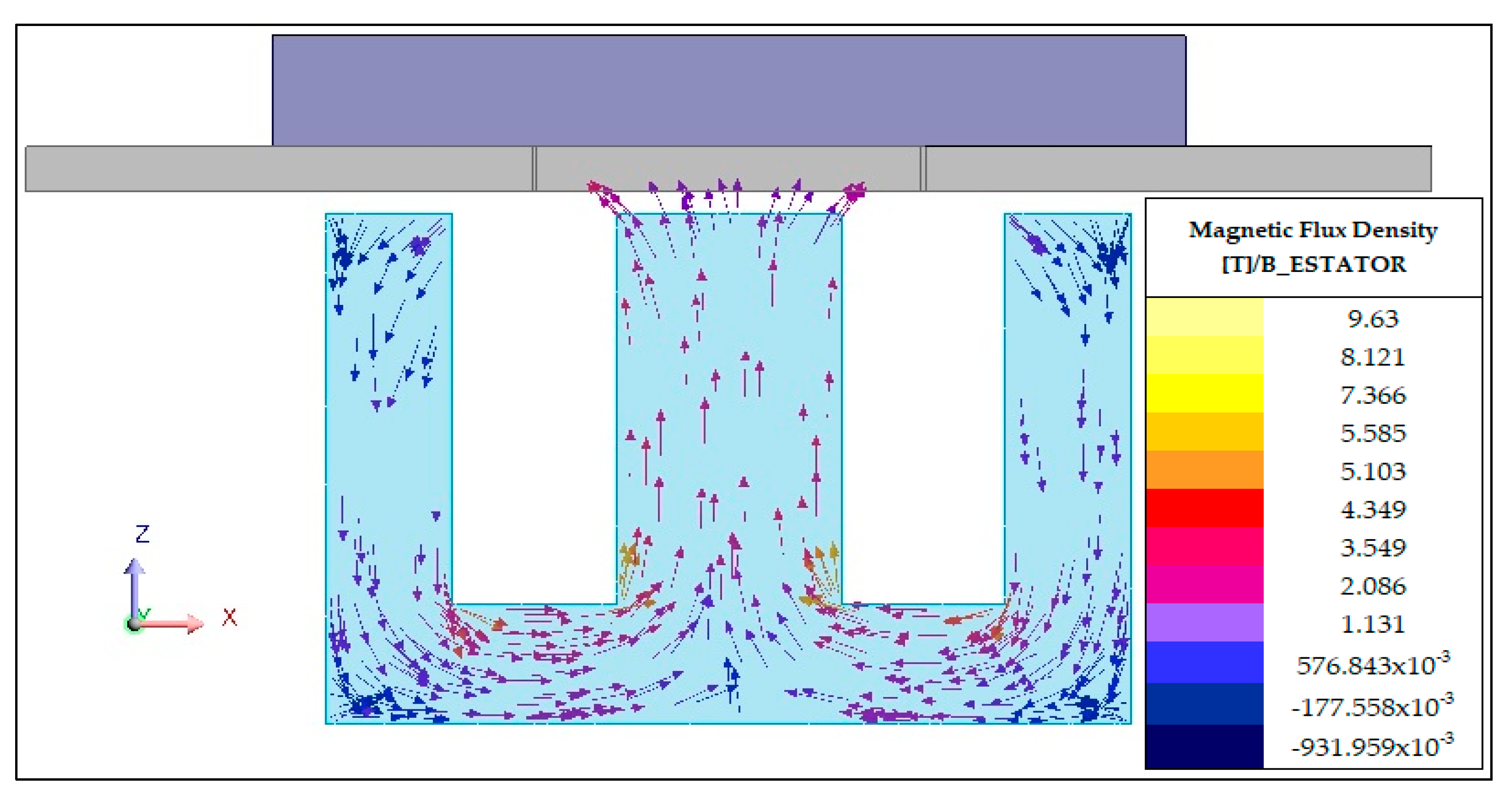
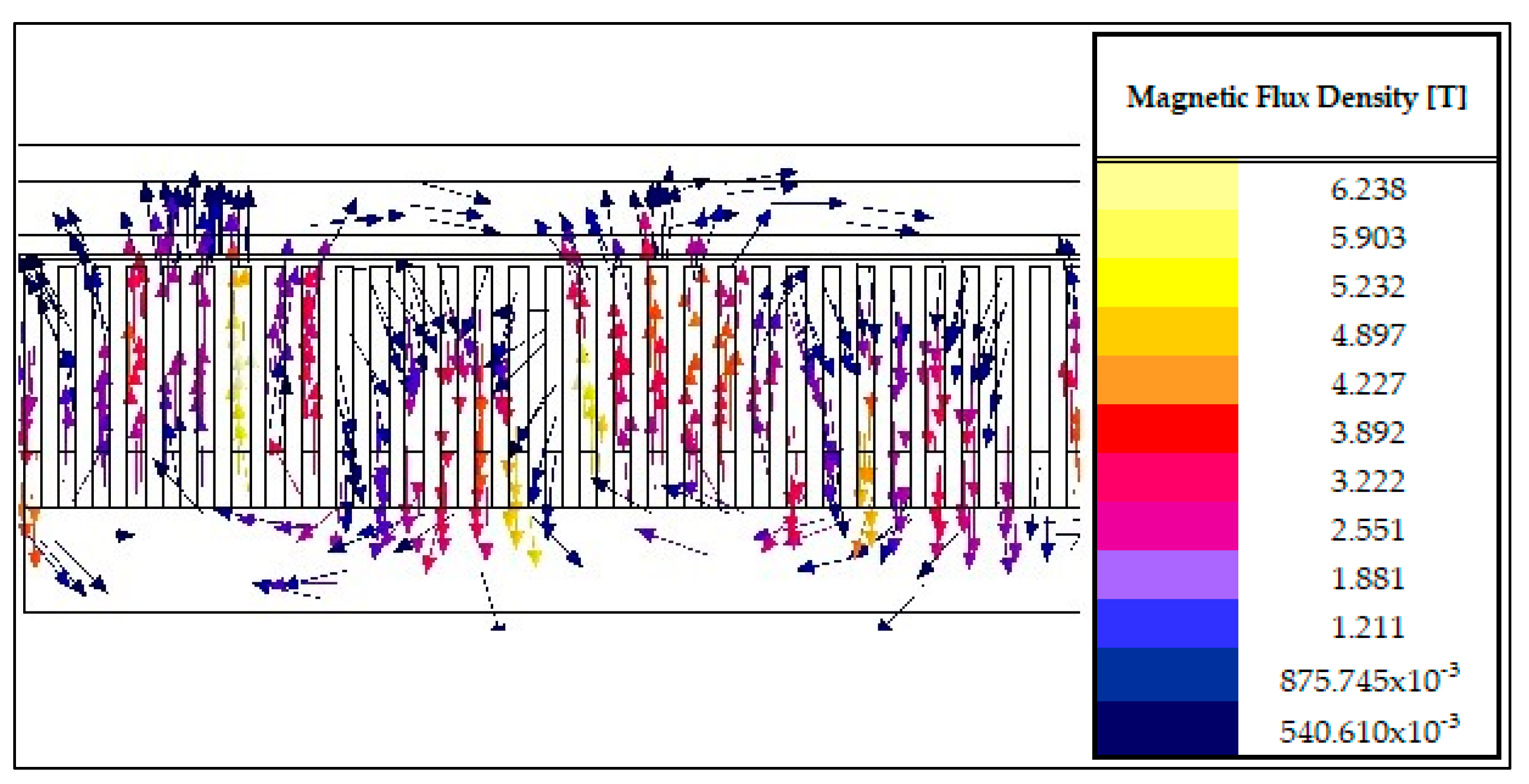
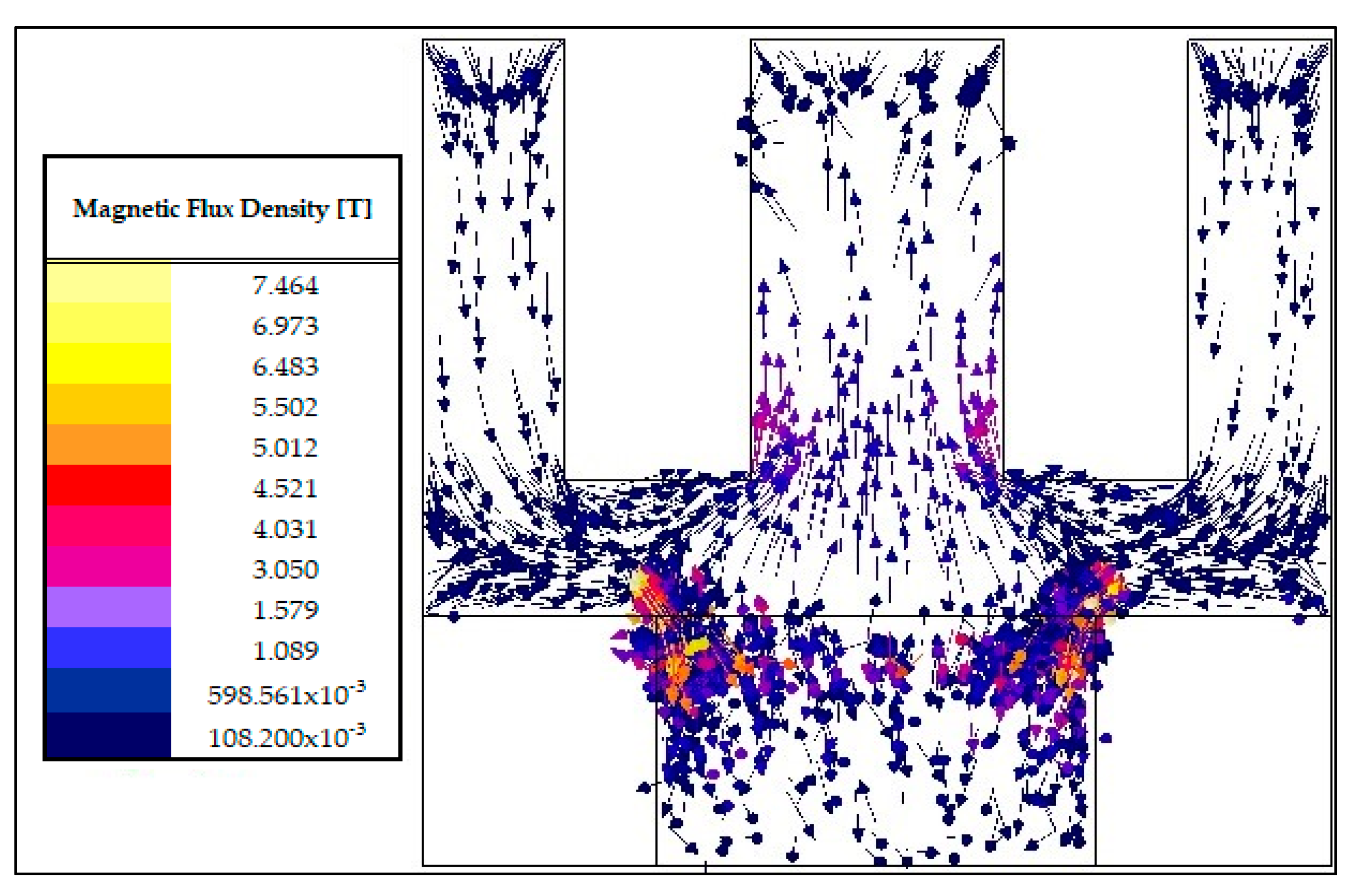
  • Figure 9 and Figure 10 show that the useful magnetic flux only operated across the transverse sections and the longitudinal magnetic flux was canceled. Equation (15) shows this configuration of the transverse magnetic flux operating into the TFLIM.
    u s e f u l T r a n v e r s a l r i g h t t e e t h l e f t t e e t h C e n t r a l t e e t h 2
    where u s e f u l is the magnetic flux that is involved in the electromechanical conversion (Wb); T r a n v e r s a l is the magnetic flux closed along transverse sections (Wb); C e n t r a l t e e t h is the magnetic flux that crosses the central teeth (Wb); r i g h t t e e t h is the magnetic flux that crosses the right-sided teeth (Wb), and l e f t t e e t h is the magnetic flux that crosses the left-sided teeth (Wb).
  • The high values reached for magnetic flux density in Figure 10 were obtained due to the linear behavior of the B-H curve that did not include the saturation effect inside the ferromagnetic regions. These values were unreachable inside real ferromagnetic steel, but the goal of this simulation was to demonstrate that the only existing magnetic flux was the transverse. To validate this simulation in an experimental test it is necessary to decrease the excitation in order to work near to the saturation zone from the B-H curve.

4.3. Simulation Results in Standstill Conditions

The results obtained from the simulations are detailed in the next subsections. These results are presented by showing the three principal magnitudes of a LIM: forces, eddy currents into the aluminum plate, and consumed electric currents.

4.3.1. Simulation of the Original Model

In this section, we describe the experiences with model 1. Figure 11 shows the principal forces in this model: thrust, levitation, and transversal. In this case, the levitation force (red line) was higher than the thrust force (blue line). If the average value of the forces was taken as a representative value of their evolution, the levitation force reached around 400 N, in comparison with the thrust force which was nearly to 80 N. It denotes that the levitation force is very important in a LIM, instead, it does not exist in a rotatory induction motor. The transverse force (green line) was not relevant in this model, its value is only 12 N, because the moving and fixed parts were aligned.
Equation (16) explains the generation of the thrust force. It is important to remark that during the simulation, the layer of iron located over the aluminum plate was assigned an electrical conductivity equal to zero, σFe = 0 S/m. Consequently, eddy currents were canceled inside this region, therefore there was no thrust force. Thus, the thrust force was only generated by the aluminum layer. The total thrust force was defined by the summation of the electromagnetic forces created over each tooth.
F y T h r u s t   F o r c e L I M = F y _ A l + F y _ F e = 0 ( σ F e = 0   S / m ) = F y _ A l { T e r m 1 :   F y _ A l _ c e n t r a l _ t e e t h > 0 T e r m 2 :   F y _ A l _ l a t e r a l _ t e e t h < 0
where F y _ A l is the thrust force in the aluminum layer (N); F y _ F e is the thrust force in the iron layer (N); F y _ A l _ c e n t r a l _ t e e t h is the positive thrust force generated by the magnetic flux that crosses the central teeth (N), and F y _ A l _ l a t e r a l _ t e e t h is the negative thrust force created by the magnetic flux that crosses the lateral teeth (N). Term 2 in Equation (15) shows the principal problem to obtain a great thrust force into the model, that is, the anti-thrust force generated over the lateral teeth. As shown in Figure 10, when the lines of the transversal magnetic flux cross the lateral teeth, they go in the opposite direction to that when they cross the central teeth. According to the Lorentz’s force [20], the negative thrust force was calculated by the vector product between the induced eddy currents and the magnetic field density into the regions of the aluminum layer located over the lateral teeth. However, over the central teeth occurred the opposite situation because there, a positive thrust force was developed, see term 1 of Equation (15). Using FEM-3D was not possible to obtain the separated contribution in the thrust force from the central and lateral teeth. In our paper, the thrust force developed corresponded to the contributions of all teeth.
Figure 12 shows the spatial distribution of the induced eddy currents inside the aluminum plate, J A l , whose values are given in A/m2. Under the motion condition of secondary part blocked we can simplify the eddy currents vector according to Equation (17) [19], where σ A l is the aluminum electric conductivity (S/m) and E the electric field (V/m). Eddy currents into the aluminum plate present only a loop along the transversal direction in x-axis.
J A l σ A l · E
Figure 13 shows the electric currents, which present an exclusive phenomenon of an LIM. Due to the finite length of the motor, the main magnetic circuit did not have a symmetry for each phase. This phenomenon is called the longitudinal end-effect. Therefore, the maximum value of the electric current will be different due to the relative position of each phase inside the primary winding. Precisely, the RMS values of the electric currents in phase A, phase B, and phase C were 84.811, 93.583, and 87.938 A, respectively.
A system where the electric currents per phase are all different (IPhase_a ≠ IPhase_b ≠ IPhase_c) is called an unbalanced three-phase system [3] and presents two relevant consequences. First, as presented in Figure 14, the spatial phasor of the magnetomotive force (MMF) was not uniform [21] because it described an ellipsoid instead of a circumference. For this reason, the instantaneous velocity of the first harmonic of the traveling magnetic wave never reached the synchronous velocity. The value of the synchronous velocity calculated in Equation (21), v S y n c h r o n o u s = 20   m / s , corresponded to its average value not to the instantaneous value. This effect produced a huge variation in the principal forces of the LIM. Second, it is important to take into account the differences among electric currents when we controlled the LIM and when the insulation of the primary winding conductors was selected.
In order to increment the thrust force, the goal of this paper was to increase term 1 and to reduce term 2 in Equation (16), by adding changes into the geometric parameters of model 1.

4.3.2. Effect of Adding Two Slots of Dielectric into the Secondary Part

Model 2 incorporated two slots into the aluminum layer (see Figure 6) with a width of 1 mm. These two new regions of air allowed for a decrease in the negative thrust force generated over the lateral teeth. With these new three regions of aluminum electrically insulated by the slots, the generated eddy currents into the aluminum layer had a different behavior with respect to model 1. Figure 15 shows the principal forces in this model. Considering their average values, the increment in the thrust force with respect to model 1 was about 20 N (an increment around 23.7%). However, the levitation force decreased to 200 N (a decrement around 49.46%).
Figure 16 presents a new distribution of eddy currents. The new slots generated new paths into the aluminum layer. Now, there were three loops of eddy currents along the x-axis. With this configuration, it was possible that over each tooth (central and lateral), the vector product between J and B generated a force along the direction of the movement, but at the same time, the levitation force decreased considerably.
Figure 17 represents the consumed electric currents in model 2. Every phase decreased approximately 2 A, compared to model 1. This effect supposes a little raise in the efficiency of the LIM.

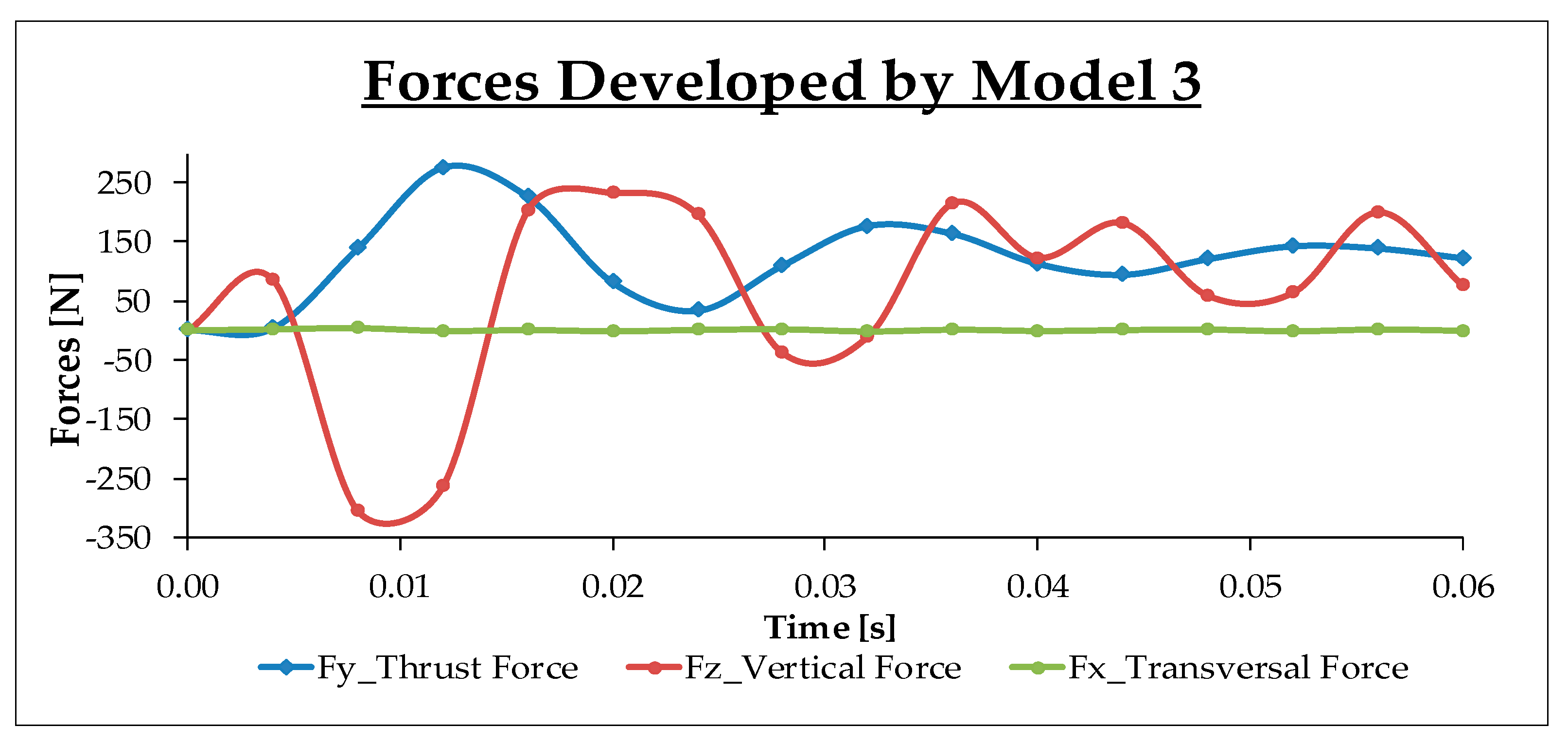
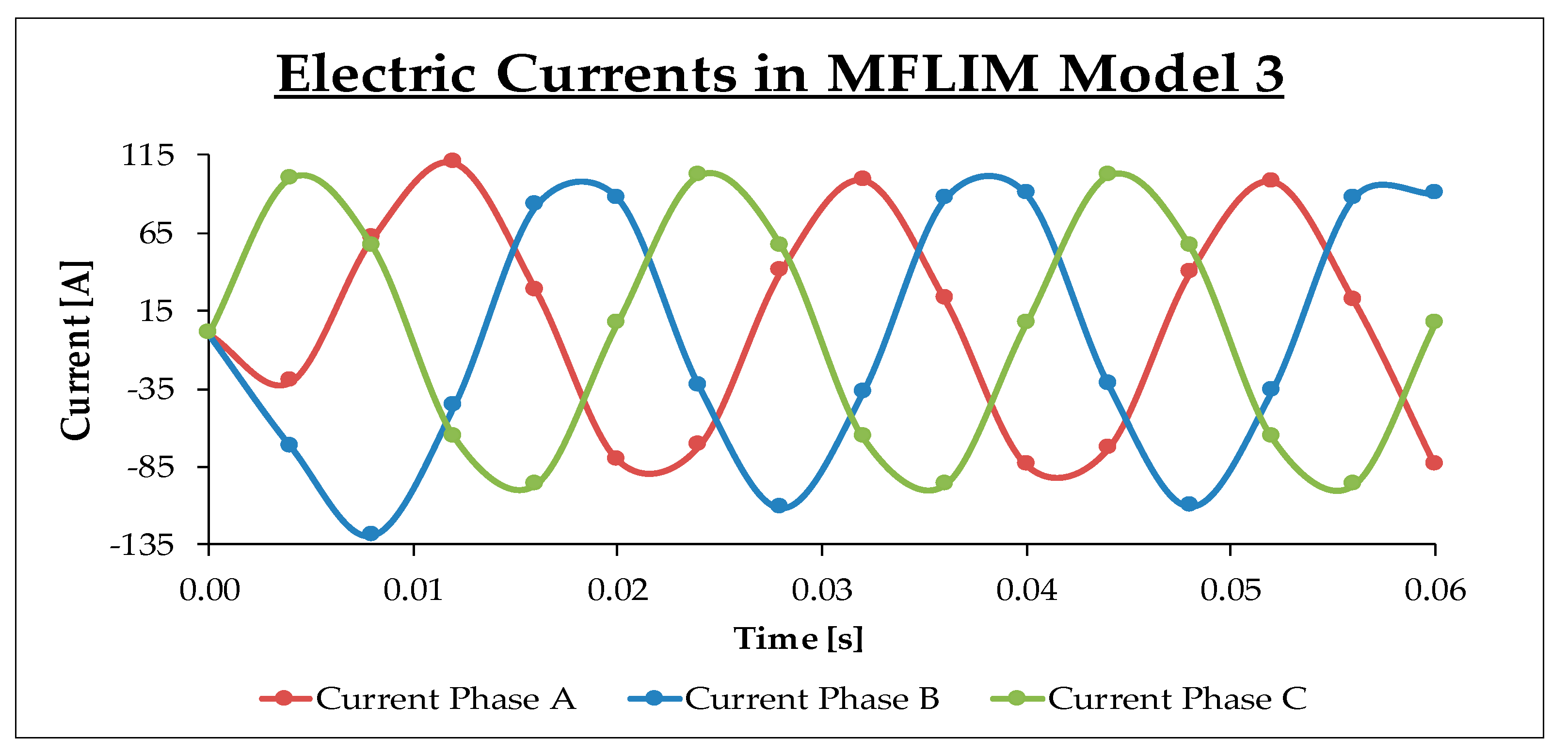
4.3.3. Effect of Adding a Ferromagnetic Yoke in the Primary Part

Model 3 developed a new strategy different from model 2. Until now, there was only a main traverse magnetic circuit. In model 3, the primary part was modified with a ferromagnetic yoke located under the central teeth (see Figure 6) in order to generate a main longitudinal magnetic circuit. With this new ferromagnetic region, the lines of the magnetic field density crossed the airgap from the primary part to the secondary part, through these two main magnetic circuits. Model 3 was called the mixed flux magnetic linear induction motor or hybrid flux magnetic linear induction motor (MFLIM). Equation (18) defines the result magnetic flux in this model:
u s e f u l = L o n g i t u d i n a l + T r a n v e r s a l
where u s e f u l is the magnetic flux involved in the electromechanical conversion (Wb); T r a n v e r s a l is the transverse magnetic flux (Wb), and L o n g i t u d i n a l is the longitudinal magnetic flux (Wb). With this new magnetic flux, the motor increased the thrust force and decreased the levitation force due to the great attraction between both parts. Figure 18 plots the principal forces in model 3. With this new primary part, the motor developed a total thrust of around 125.054 N. This value represents a wide increment with respect to models 1 and 2. In relative terms, the thrust force raised around 56.2% in respect to model 1 and around 26.6% compared to model 2. The attraction between both parts increased, so the levitation force reached a value of 65.383 N, which implied a decrement of 84%.
Figure 19 shows another advantage of model 3, that is, the reduction of the consumed electric currents. Approximately, the value of these currents was around 15% smaller than in model 1.
In model 3, the combined action of both magnetic fluxes generated the maximum thrust force obtained in all proposed models. Figure 20 and Figure 21 illustrated the longitudinal and transverse paths for the magnetic field density.
In conclusion, model 3 included two different phenomena. First, the effect of the incorporation of the two slots into the aluminum layer, which generated a great thrust force. Second, the introduction of the ferromagnetic yoke under the central teeth, which was a correct way to create an LIM with a mixed or hybrid magnetic flux configuration.

4.3.4. Effect of Varying the Width of the Transversal Slots

Model 4 redesigns the width of the transversal slots of the primary part increasing its dimension along the x-axis (see Figure 7). To this end, a sweep parameter was used which found the optimal value of this dimension. This change into the opening of the transversal slots was necessary to show how the thrust force increased and the electric field over the lateral teeth decreased when the opening of the slot increased. The initial value of the transversal slots was 35 mm (see Figure 2) and the final value was 75 mm. Figure 22 shows the thrust force for the different openings in a transitory state. As shown, the thrust force did not change significantly.
To study the evolution of the forces for each dimension of the transversal slots, the average values of Fy are summarized in Table 3. Besides, this table contains the average values obtained with model 3, whose results are a reference value. Model 4 incorporated all changes from models 2 and 3.
Figure 23 collects all data from Table 3. The optimal thrust force was reached in model 4 for an increment of 20 mm in the transversal slots. This force was around 138 N and consequently, the opening of the transversal slots has been redefined with a value of 55 mm. Compared to model 3, the thrust force represents an improvement of around 10%. Not all increments of the transversal slots were valid to improve the thrust force because with an increment greater than 20 mm the leakage flux began to be relevant, and the linkage magnetic flux fell.
The levitation force presented the opposite behavior when the transversal slots increased. If model 3 was considered as a reference value, with the new dimension of the transversal slots fixed in 55 mm, model 4 operated under conditions of attraction forces as shown in Figure 24. Figure 25 plots the average values for this attraction force. Moreover, the evolution of Fz did not present an optimum value when the transversal slots were increased 20 mm in contrast with the thrust force. For this value, model 4 developed an average attraction force of −56.445 N.

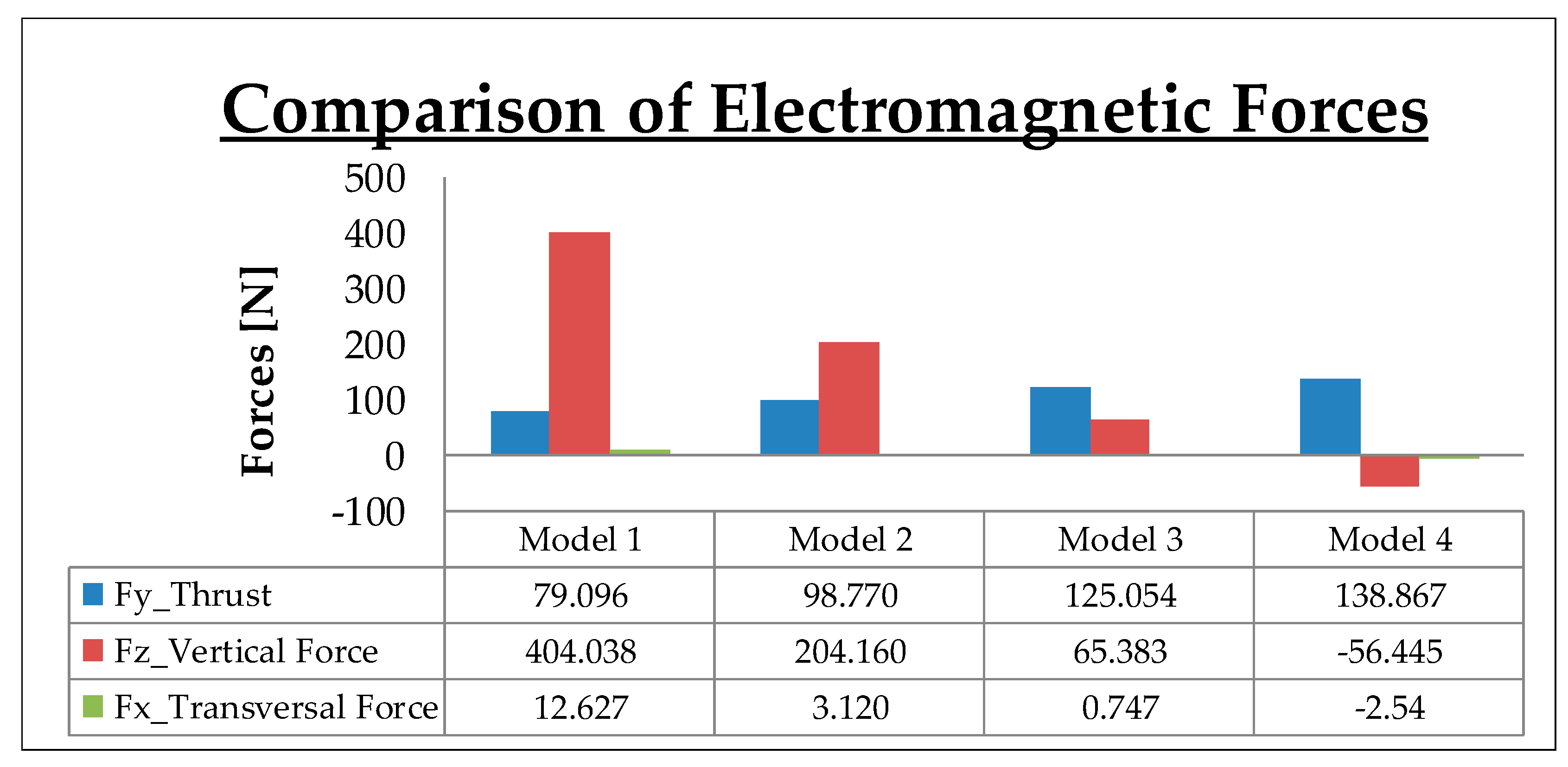
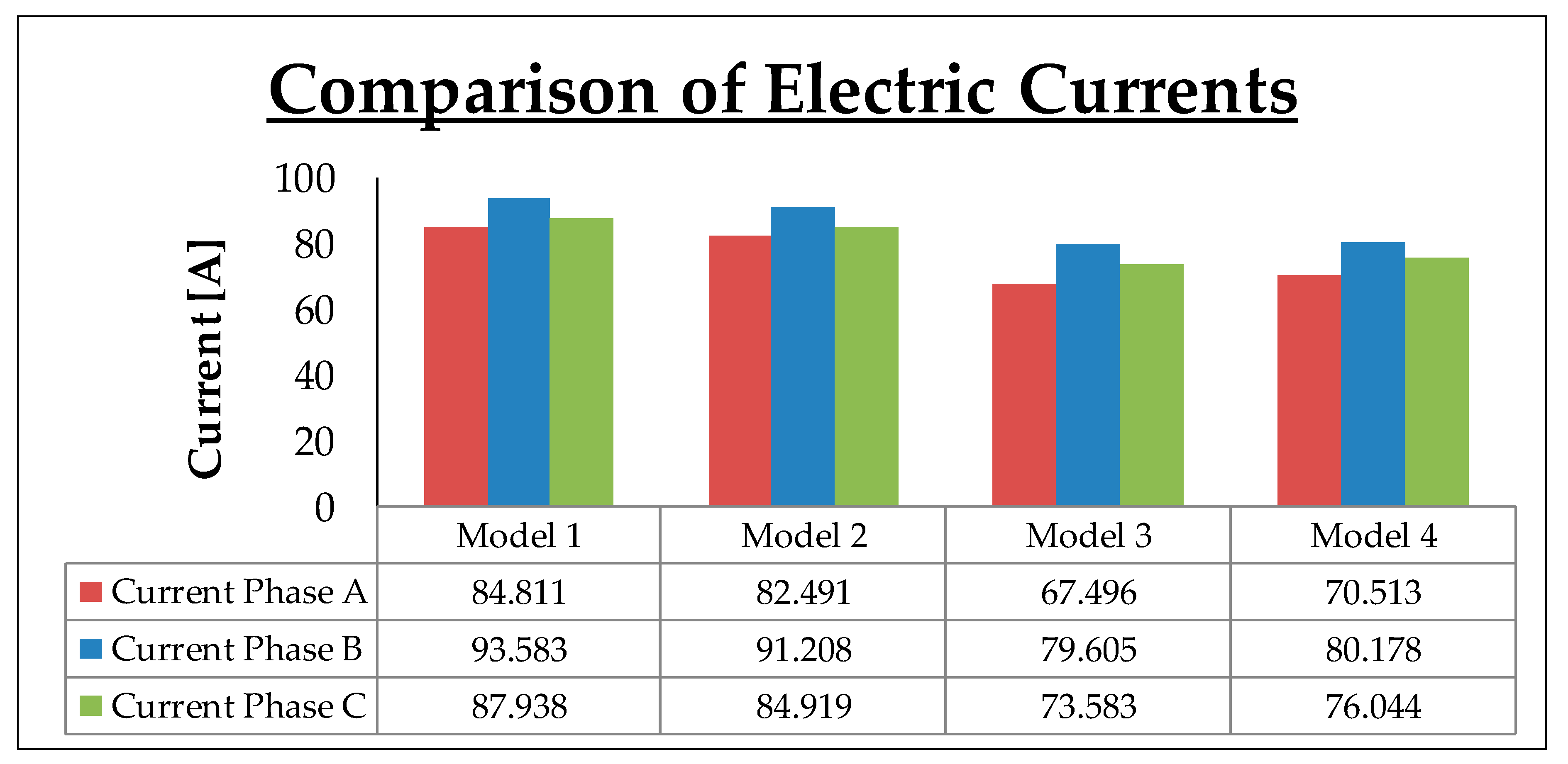
4.3.5. Comparative Study of the Main Results Obtained in Standstill Conditions

In this section, a comparative study between all models is presented. Figure 26 and Figure 27 show the evolution of the thrust and levitation forces for each model. For model 4, an opening of the transversal slots equal to 55 mm was considered. Each model developed a thrust force greater than the previous model. For the dynamic conditions imposed (s = 1), the levitation force presented a great change in each model. In conclusion, one can say that an improvement in the thrust force implied a reduction in the levitation force. In fact, in model 4, the levitation force changed from the levitation condition to attraction.
The dynamic evolution of the forces is important to design a control strategy over an MFLIM. All models presented a similar transitory state with a maximum value of the thrust force in the interval time (0.010–0.012 s). Figure 28 shows the average value of the principal forces in each model. The transversal force along the x-axis was not relevant, although this component cannot be neglected because an LIM can develop a motion through a curve path.
Figure 29 represents the consumed electric currents in all models. The obtained results of each model showed that the electric currents always present the same behavior, see Equation (19):
I P h a s e _ a < I P h a s e _ c < I P h a s e _ b
The current linked to phase B was higher than the currents in other phases with a maximum value in model 1 around 93.5 A. Instead, phase A always presented the most efficient current phase with only 67.496 A in model 3. The electric current associated with phase C had an intermediate value between the others in all experiences. In order to design the dimensions of the copper wire and the rest of the devices that protect the MFLIM, the current of phase B was a reference signal. Model 3 implied a reduction of the currents consumed per phase with respect to the initial model around 20.5% (phase A), 15% (phase B), and 16.3% (phase C). The developed models illustrated the great relevance of the location of the coils of each phase inside the armature winding and showed also that the changes introduced into the geometry are very important for the consumed electric current.

4.4. Simulation Results with Motion
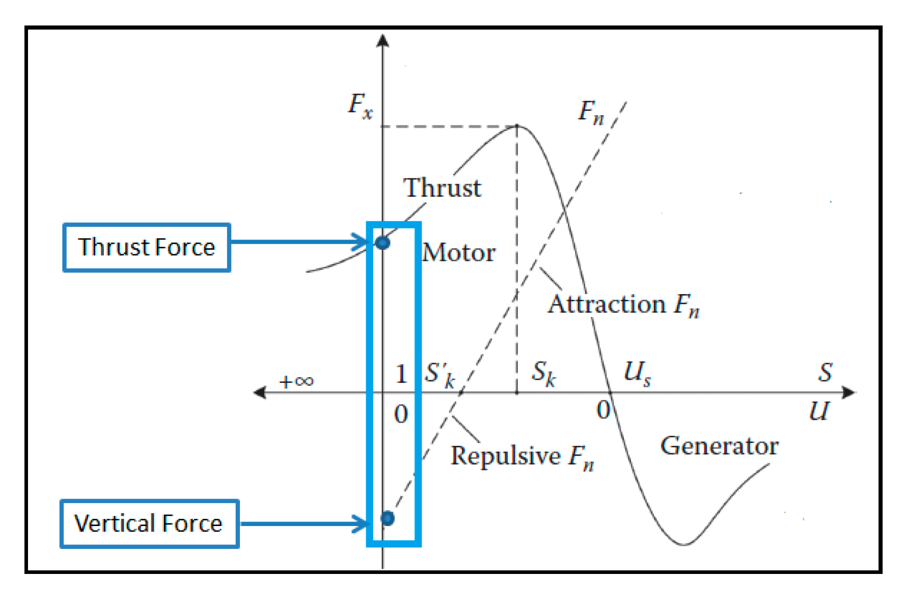
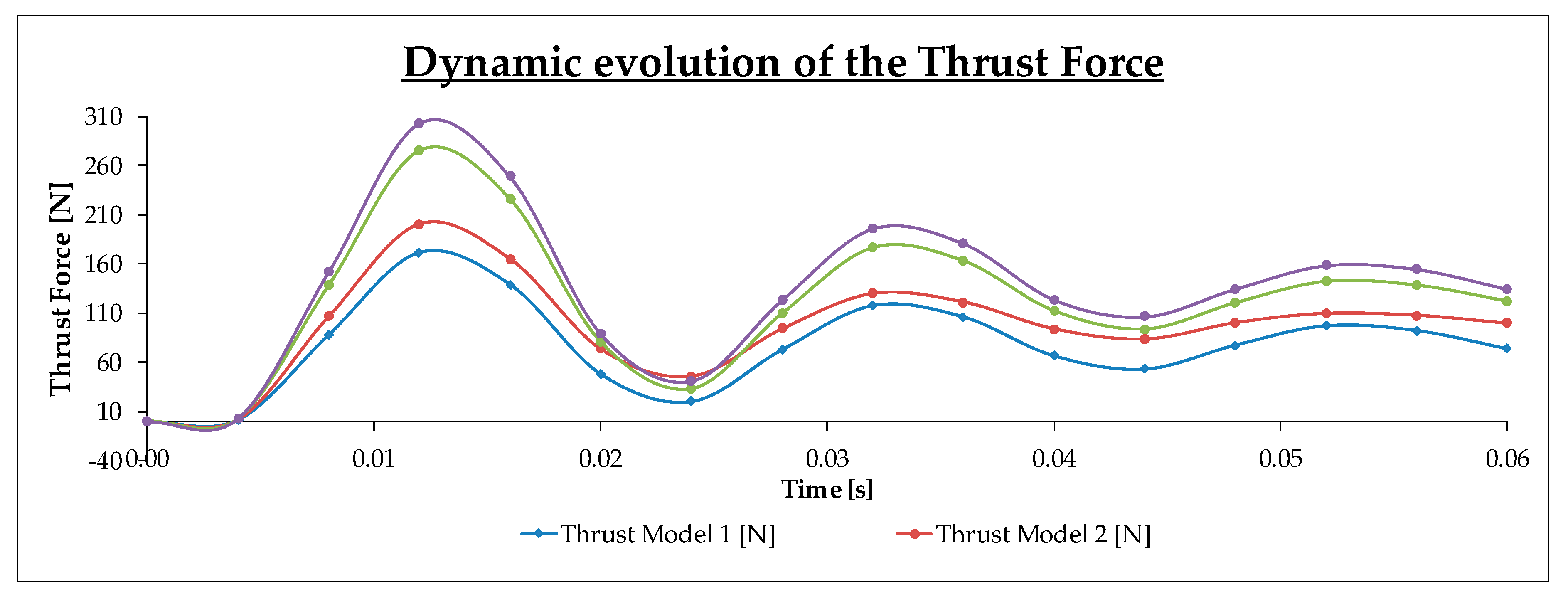
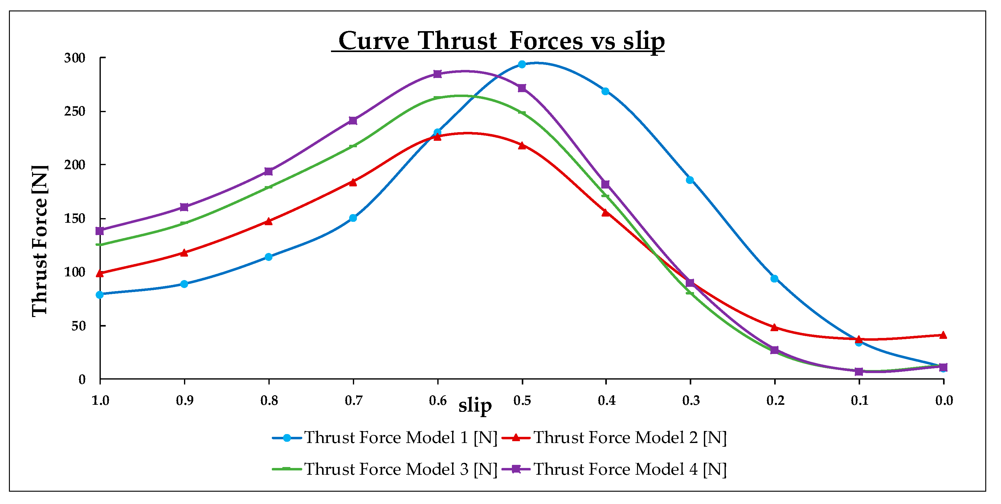
To determine the influence of the motion in the proposed models, in this section, it is presented the FEM-3D simulation of the models including motion in the moving parts. Thus, Table 4 shows the velocities and its corresponding slips (see Equation (2)) selected to study the effect of the motion in the analyzed models. More specifically, we analyze the thrust force, the levitation force, and the electric currents. It is important to notice that the friction losses are not taken into account in the present work.
Figure 30 shows the evolution of the thrust force of each model for all values shown in Table 4. To understand this figure, it is necessary to consider the following regions inside:
  • Region I (low velocities zone): 0.6 < s < 1 0 m s < v m o v i n g _ p a r t < 8 m s . With these velocities, the behavior of the thrust force had the same evolution as in standstill conditions, where this force obtained its highest value in model 4 (see Equation (20)).
    F y _ m o d e l _ 4 > F y _ m o d e l _ 3 > F y _ m o d e l _ 2 > F y _ m o d e l _ 1
Between this range of slips, the developed thrust forces for each model increased their values until the slip reached the value of 0.6. At this point, the thrust forces from model 2, model 3, and model 4 reached their maximum value around 226.2, 262.447, and 284.778 N, respectively.
  • Region II (Medium velocities zone): 0.5 < s < 0.6 8 m s < v m o v i n g _ p a r t < 10 m s .
    This region was characterized by a non-uniformity evolution of the thrust force. Model 2, model 3, and model 4 presented their inflection points between these velocities and after that continued with an evolution similar to region I (see Equation (21)).
    F y _ m o d e l _ 4 > F y _ m o d e l _ 3 > F y _ m o d e l _ 2
    However, the thrust force developed in model 1 continued to increase from 8 to 10 m/s, where the thrust force was nearly 294 N (with a slip around 0.5). This value was the highest thrust force obtained in the present work.
  • Region III (High velocities zone): 0 < s < 0.5 10 m s < v m o v i n g _ p a r t < 20 m s .
    In this region, the evolution of the thrust force decreased in all models. In general, model 1 presented a higher thrust force than others. The behavior of these forces in model 2, model 3, and model 4 were very similar. The thrust forces decreased as the velocity of the secondary part reached the synchronous velocity (20 m/s and s = 0), when model 2 developed the highest thrust force (around 41 N) at slip equal to zero. This phenomenon appeared due to the end-effect and it was not present in asynchronous rotatory machines because the torque obtained at synchronous velocity was equal to zero.
Next, Figure 31 shows the effect of the motion for the levitation force. This figure gives us the following information:
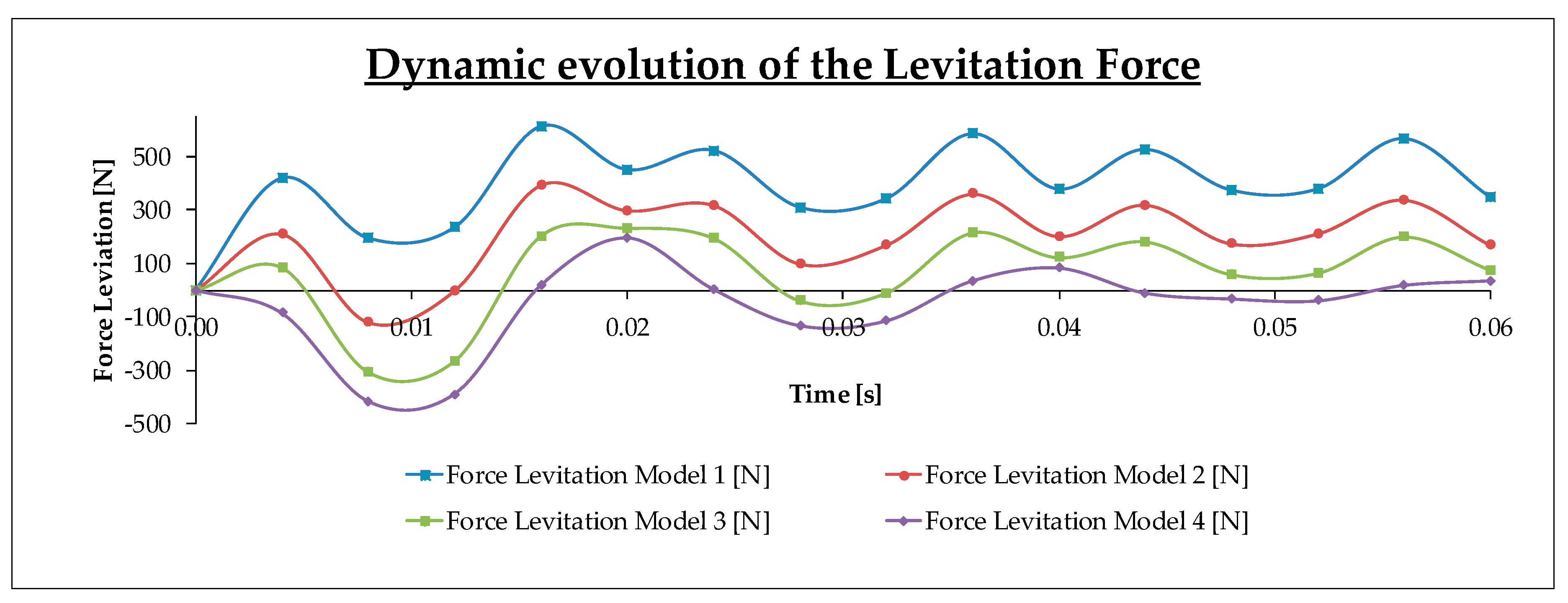
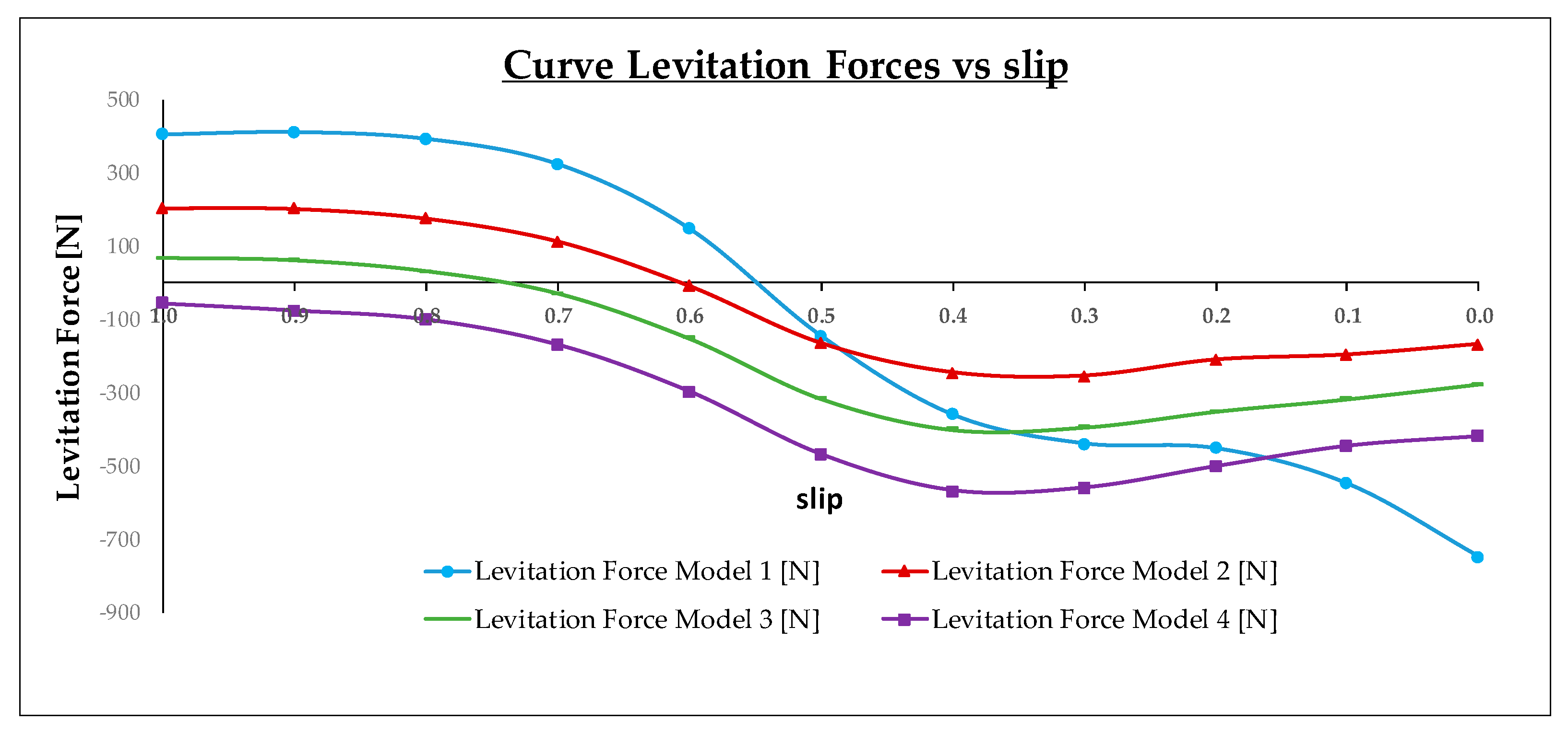
  • Model 1, model 2, and model 3 presented two regions of work depending on the selected slip. The change-point between the levitation zone and the attraction zone varied in the function of the models. So, this change of zone occurred when the values of slips were 0.55 in model 1, 0.6 in model 2, and 0.72 in model 3. However, model 4 did not operate under levitation condition. For all slip values, model 4 developed an attraction force that reached the maximum value near to 568 N with a velocity equal to 12 m/s (slip equal to 0.4).
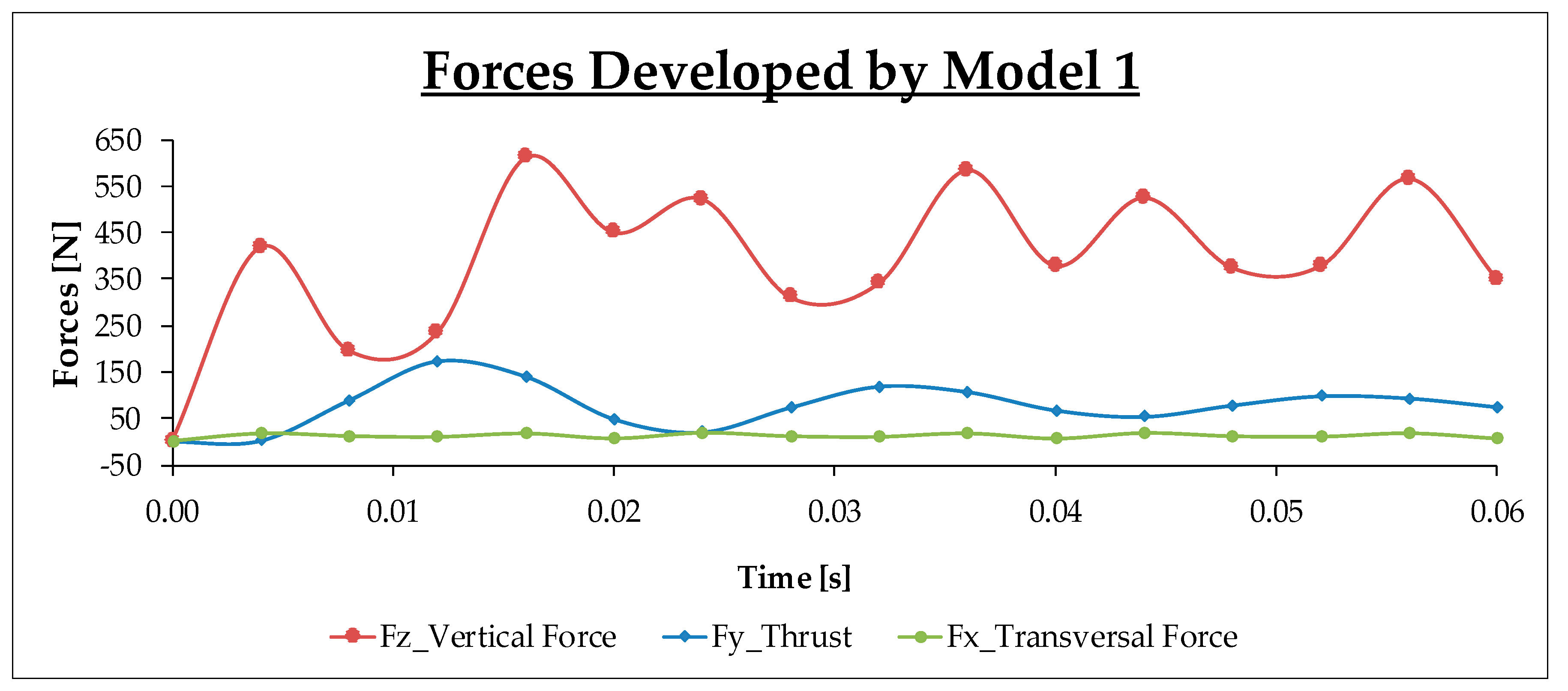
  • Two regions are shown in Figure 31: Region I: 0.5 < s < 1 0 m s < v m o v i n g _ p a r t < 10 m s . Inside this region, the behavior of the levitation force is given by Equation (22) and followed the same law as in the standstill conditions. Besides, at slip equal to one, model 1, model 2, and model 3 developed the maximum levitation force around 404.04, 204.16, and 65.38 N, respectively:
    F z _ m o d e l _ 4 < F z _ m o d e l _ 3 < F z _ m o d e l _ 2 < F z _ m o d e l _ 1
    It is important to remark the relevance of this force in the TFLIM. The highest values of levitation and attraction forces were obtained in model 1 (around 404.04 N for slip equal to one and −747.63 N, with velocities near to the synchronous velocity or slip equal to zero).
    Region II: 0 < s < 0.5 10 m s < v m o v i n g _ p a r t < 20 m s . In this zone, model 2, model 3, and model 4 continued the evolution from region I (see Equation (23)). These forces did not continue decreasing with the slip as occurred with the levitation force from model 1, F z _ m o d e l _ 1 , that decreased with the slip.
    F z _ m o d e l _ 4 < F z _ m o d e l _ 3 < F z _ m o d e l _ 2
Figure 32, Figure 33 and Figure 34 show the evolution of the electrical current for each phase. These figures confirm the reached results in standstill conditions.
For each model, the relationship between the electric currents followed Equation (17). Besides, model 3 was the configuration that presented a low electric current consumed by each phase across the range of velocities. So, with a slip of 0.5, phase A and phase C in model 3 only consumed 66.14 and 70.60 A, respectively. Phase B reached its minimum value with a slip value of 0.3 (around to 75.55 A).
If we compare the obtained results considering the whole range of slips from Figure 30, Figure 31, Figure 32, Figure 33 and Figure 34, we have available a great amount of information about the convenience to include the proposed changes into the geometry of the TFLIM, in order to achieve a more efficient motor. We can conclude that with slip values above 0.5, model 4 developed the highest thrust force. It supposes that the changes included in the geometric parameters are useful to increase the thrust force inside the range of velocities between 0 and 10 m/s. However, model 4 always operated under attraction force condition, so an increment in the thrust force implied a reduction in the levitation force. In this way, the thrust force developed by model 3 was near to model 4 and it operated inside the levitation zone for low velocities. Therefore, we can say that model 3 is an optimum model to operate with velocities below 10 m/s. However, for slip values below 0.5, model 1 presents the best behavior. In conclusion, the proposed changes are irrelevant for velocities from 10 to 20 m/s and model 3 is the most efficient configuration for all range of velocities in comparison with model 1, that presents in phase B, the highest electric current consumed, around 95 A at the synchronous velocity.

5. Conclusions

The main goal of this paper was to develop a new configuration for a more efficient LIM, based on a prototype model called model 1. To this end, we proposed three changes to the geometric parameters of the fixed and moving parts and we defined a new model for each proposed change. The first change was incorporated into model 2, including three different regions into the aluminum layer through two slots of dielectric, in order to separate the loops of the induced currents. Thus, the thrust force generated over the lateral teeth was developed in the desired direction. The second change was proposed in model 3, where we included a ferromagnetic yoke in the primary part to produce a longitudinal magnetic flux. Finally, the third change was included in model 4 and implied the optimization of the width of the transversal slots.
In standstill conditions (slip = 1), model 4 achieved the maximum thrust force of all models, around 75% with respect to the prototype model (model 1). However, this model presented a great disadvantage because it produces a loss of levitation force which begins to operate inside an attraction zone. With motion and velocities below 10 m/s (slip > 0.5), model 4 also developed the maximum thrust force. However, for velocities between 10 and 20 m/s (slip < 0.5), the changes added into the geometry did not contribute to increasing the thrust force. In this case, model 1 developed the maximum thrust force. Besides, for the whole range of analyzed velocities, model 4 operated inside the attraction zone. Hence, for velocities below 10 m/s (slip > 0.5), model 3 presented a similar thrust force as model 4 and operated inside the levitation zone for velocities below 6 m/s (slip > 0.7).
Regarding the consumed electric currents, model 3 presented the most efficient configuration for all slip values because it achieved two main magnetic circuits operating inside the motor—transversal and longitudinal. In brief, for velocities below 10 m/s, model 3 represents an improvement in respect to model 1, due to the high thrust force developed and the low electric current consumed.
To simulate all proposed models with FEM-3D, we presented a method that allows one to analyze the magnetic field density along the airgap in an LIM. The method is composed of two steps. First, according to an analytical method, the first harmonic of the magnetic field density in the airgap was computed. This is the starting point of the simulations with FEM-3D. Second, with an iterative process, the external circuit coupling to supply the LIM was fixed. To this end, we used two electrical parameters: the number of turns of the coils per phase, Nphase, and the level of voltage in an AC three-phase system, VLINE. Using FEM-3D, the coupling between the primary winding of the LIM and the voltage sources has been defined completely. In addition, the selected transitory state in FEM-3D gives us valuable information to design a control strategy of a LIM.
In the transitory state, the use of FEM-3D allows us to analyze the unbalanced system originated by the longitudinal end-effect. It is a phenomenon that cannot be neglected and presents the same distribution for all models and values of slip: IPhase_a < IPhase_c < IPhase_b. This behavior implies a great advantage of using FEM-3D for two reasons. Firstly, the highest phase (Ib) will be a reference signal to design the insulated scheme and the electrical protection of the LIM. Secondly, the unbalanced electric system supposes high variations in the forces during the transitory state. This effect implies that it is necessary to carry out an analysis of the vibration modes using FEM when we want to design the structural support of an LIM in mechanical engineering.

Author Contributions

All authors have collaborated in the writing of the paper. J.A.D.H. has made the design and simulation of all experiments and prepared the original draft presentation. N.D.C. and E.G.V. collaborated in the supervision of the work and in the review and editing of the draft. All authors have read and agreed to the published version of the manuscript.

Funding

This work was supported in part by the Spanish Ministry of Economy and Competitiveness under the Projects CICY DPI2017-84259-C2-2-R, PID2019-108377RB-C32, and the group of educational innovation project GID2016-6.

Conflicts of Interest

The authors declare no conflict of interest.

References

  1. Nasar, S.N.; Boldea, I. Linear Motion Electric Machine; Wiley-Interscience Publication: Hoboken, NJ, USA, 1976; ISBN 0471630292. [Google Scholar]
  2. Han, H.S.; Kim, D.S. Magnetic Levitation. Maglev Technology and Applications; Springer: New York, NY, USA, 2016. [Google Scholar]
  3. Gieras, J.F. Linear Induction Drives; Clarendon Press: Oxford, UK; New York, NY, USA, 1994. [Google Scholar]
  4. Laithwaite, E.R. Induction Machines for Special Purposes; Chemical Publishing Company Inc.: New York, NY, USA, 1966; ISBN 978-0600411475. [Google Scholar]
  5. Luo, J.; Kou, B.; Zhou, Y.; Zhang, L. Analysis and design of an E-core transverse-flux flux-reversal linear motor. In Proceedings of the 19th International Conference on Electrical Machines and Systems (ICEMS), Chiba, Japan, 13–16 November 2016; pp. 1–5. [Google Scholar]
  6. Darabi, S.; Beromi, Y.A.; Izadfar, H.R. Comparison of two common configurations of LSRM: Transverse flux and longitudinal flux. In Proceedings of the International Conference and Exposition on Electrical and Power Engineering, Iasi, Romania, 25–27 October 2012; pp. 451–455. [Google Scholar] [CrossRef]
  7. Palomino, G.G.; Conde, J.R. Ripple reduction in a PMLSM with Concentrated Winding using 2-D finite elements simulation. In Proceedings of the 4th IET Conference on Power Electronics, Machines and Drives, York, UK, 2–4 April 2008; pp. 451–454. [Google Scholar] [CrossRef]
  8. Nozaki, Y.; Baba, J.; Shutoh, K.; Masada, E. Improvement of transverse flux linear induction motors performances with third order harmonics current injection. IEEE Trans. Appl. Supercond. 2004, 14, 1846–1849. [Google Scholar] [CrossRef]
  9. Cuong, N.V.; Koseki, T.; Isobe, E. Numerical analysis for the influence of the construction of the secondary reaction plate on the characteristics of linear induction motor. In Proceedings of the IECON 2013—39th Annual Conference of the IEEE Industrial Electronics Society, Vienna, Austria, 10–13 November 2013; pp. 3012–3017. [Google Scholar] [CrossRef]
  10. Isfahani, A.H.; Ebrahimi, B.M.; Lesani, H. Design Optimization of a Low-Speed Single-Sided Linear Induction Motor for Improved Efficiency and Power Factor. IEEE Trans. Magn. 2008, 44, 266–272. [Google Scholar] [CrossRef]
  11. Park, S.C. Thrust and attraction force calculation of a linear induction motor with the moving cage-type secondary. In Proceedings of the Sixth International Conference on Electrical Machines and Systems, Beijing, China, 9–11 November 2003; Volume 1, pp. 226–229. [Google Scholar]
  12. Lee, B.; Koo, D.; Cho, Y. Investigation of Linear Induction Motor According to Secondary Conductor Structure. IEEE Trans. Magn. 2009, 45, 2839–2842. [Google Scholar] [CrossRef]
  13. Kwon, B.I.; Woo, K.I.; Kim, S.; Park, S.C. Analysis for dynamic characteristics of a single-sided linear induction motor having joints in the secondary conductor and back-iron. IEEE Trans. Magn. 2000, 36, 823–826. [Google Scholar] [CrossRef]
  14. Li, Z.; Yu, X.; Xue, Z.; Sun, H. Analysis of Magnetic Field and Torque Features of Improved Permanent Magnet Rotor Deflection Type Three-Degree-of-Freedom Motor. Energies 2020, 13, 2533. [Google Scholar] [CrossRef]
  15. Escarela-Perez, R.; Melgoza, E.; Alvarez-Ramirez, J.; Laureano-Cruces, A.L. Nonlinear time-harmonic finite-element analysis of coupled circuits and fields in low frequency electromagnetic devices. Finite Elem. Anal. Des. 2010, 46, 829–837. [Google Scholar] [CrossRef]
  16. Rivas, J.J.M. Estudio de la Interacción Magneto-Eléctrica en el Entrehierro de los Motores Lineales de Inducción de Flujo Transversal. Aplicación al Diseño de un Prototipo para Tracción Ferroviaria de tren Monoviga. Ph.D. Thesis, Universidad Politécnica de Madrid, Madrid, Spain, 2003. [Google Scholar]
  17. Boldea, I. Linear Electric Machines, Drives, and MAGLEV’s Handbook; CRC Press: Boca Raton, FL, USA, 2013. [Google Scholar]
  18. Boldea, I.; Nasar, S.A. The Induction Machine Handbook; CRC Press: Boca Raton, FL, USA, 2002. [Google Scholar]
  19. Turoswski, J.; Turoswski, M. Engineering Electrodynamics. Electric Machine, Transformer and Power Equipment Design; CRC Press: Boca Raton, FL, USA, 2016. [Google Scholar]
  20. Jezierski, E. Transformer. Theory; WNT: Warsaw, Poland, 1975. [Google Scholar]
  21. Gieras, J.F. Electrical Machines. Fundamentals of Electromechanical Energy Conversion; CRC Press, Taylor & Francis Group: Boca Raton, FL, USA, 2017. [Google Scholar]
  22. Lipo, T.A. Introduction to AC Machine Design; IEEE Press Series on Power Engineering; Wiley: Hoboken, NJ, USA, 2017. [Google Scholar]
Figure 1. Electromagnetic forces in a linear induction motor (LIM).
Applsci 10 07004 g001
Figure 2. Dimensions of a ferromagnetic sheet (mm) [16].
Applsci 10 07004 g002
Figure 3. Three-dimensional view of model 1.
Applsci 10 07004 g003
Figure 4. Scheme of the AC three-phase winding with four layers.
Applsci 10 07004 g004
Figure 5. Curve forces versus slip in an LIM [18].
Applsci 10 07004 g005
Figure 6. Changes included in models 2 and 3.
Applsci 10 07004 g006
Figure 7. Transversal slots incremented from 10 to 40 mm [16].
Applsci 10 07004 g007
Figure 8. Simulation conditions imposed during the simulation.
Applsci 10 07004 g008
Figure 9. Distribution of the magnetic field density along the airgap.
Applsci 10 07004 g009
Figure 10. Transversal view of magnetic flux in model 1.
Applsci 10 07004 g010
Figure 11. Forces in model 1.
Applsci 10 07004 g011
Figure 12. Spatial distribution of eddy currents in model 1.
Applsci 10 07004 g012
Figure 13. Electric current per phase in model 1.
Applsci 10 07004 g013
Figure 14. MMF generated by an unbalanced system of electric currents [21].
Applsci 10 07004 g014
Figure 15. Forces in model 2.
Applsci 10 07004 g015
Figure 16. Spatial distribution of eddy currents in model 2.
Applsci 10 07004 g016
Figure 17. Electric current per phase in model 2.
Applsci 10 07004 g017
Figure 18. Forces in model 3.
Applsci 10 07004 g018
Figure 19. Electric current per phase in model 3.
Applsci 10 07004 g019
Figure 20. Longitudinal magnetic field density.
Applsci 10 07004 g020
Figure 21. Transverse magnetic field density.
Applsci 10 07004 g021
Figure 22. Thrust force in a transitory state for different values of the transversal slots.
Applsci 10 07004 g022
Figure 23. Thrust forces versus an increment of the transversal slots.
Applsci 10 07004 g023
Figure 24. Levitation force in the transitory state with different values of the transversal slots.
Applsci 10 07004 g024
Figure 25. Levitation forces versus increment of transversal slots.
Applsci 10 07004 g025
Figure 26. Dynamic evolution of the thrust force in each model.
Applsci 10 07004 g026
Figure 27. Dynamic evolution of the levitation force in each model.
Applsci 10 07004 g027
Figure 28. Comparison of the principal forces in each model.
Applsci 10 07004 g028
Figure 29. Electric currents per phase in each model.
Applsci 10 07004 g029
Figure 30. Thrust force versus slips.
Applsci 10 07004 g030
Figure 31. Levitation force versus slips.
Applsci 10 07004 g031
Figure 32. Electric current phase A versus slips.
Applsci 10 07004 g032
Figure 33. Electric current phase B versus slips.
Applsci 10 07004 g033
Figure 34. Electric current phase C versus slips.
Applsci 10 07004 g034
Table 1. Main geometric parameters of the LIM.
Geometric Parameters of the LIM (mm)
Thickness Al.Thickness Fe.Width Al.Width Fe.Length Al.Length Fe.
1025300195990970
Mechanic Airgap: g5
Width Longitudinal Slot8.5
Slot Pitch16.5
Length Fixed Part503.5
Table 2. Electrical and magnetic properties.
Electrical and Magnetic Properties of the
Materials Esed in FEM-3D
Aluminum
Conductivity (Sm–1)3.73 × 10⁷
Relative Permeability1
Steel
Conductivity (Sm–1)0
Relative Permeability2500
Copper
Resistivity (Ωmm2/m)2.37 × 10–2
Relative Permeability1
Table 3. Average value of thrust force and levitation force.
Final Width of the Transversal Slots (mm)Fy_Thrust Force (N)Fz_Levitation Force (N)
45 mm (Increment of 10 mm)132.888−13.704
55 mm (Increment of 20 mm)138.867−56.445
65 mm (Increment of 30 mm)136.854−96.439
75 mm (Increment of 40 mm)135.479−136.308
Model 3
(Reference Values)
125.05465.383
Table 4. Slips values and linear velocities simulated with FEM-3D.
Dynamic Conditions for the Motion Analysis
Slip00.10.20.30.40.50.60.70.80.91
Velocity (m/s)20181614121086420

