

Comparative Numerical Study on the Weakening Effects of Microwave Irradiation and Surface Flux Heating Pretreatments in Comminution of Granite

Abstract
:1. Introduction
2. Rock Constitutive Model
2.1. Bi-Surface Viscoplastic Consistency Model
2.2. Damage Formulation and Combining the Damage and Viscoplastic Parts
2.3. Stress Integration of Rock Constitutive Model
| Algorithm 1 Solution process for elemental stresses |
|
3. Simulation Method for Microwave Heating Induced Failure
3.1. Strong Form of the Uncoupled Electromagnetic–Thermo-Mechanical Problem
3.1.1. Formulation of the Electromagnetic Problem
3.1.2. Formulation of the Thermo-Mechanical Problem
3.2. Finite Element Discretized Form for the Uncoupled Thermo-Mechanical Problem
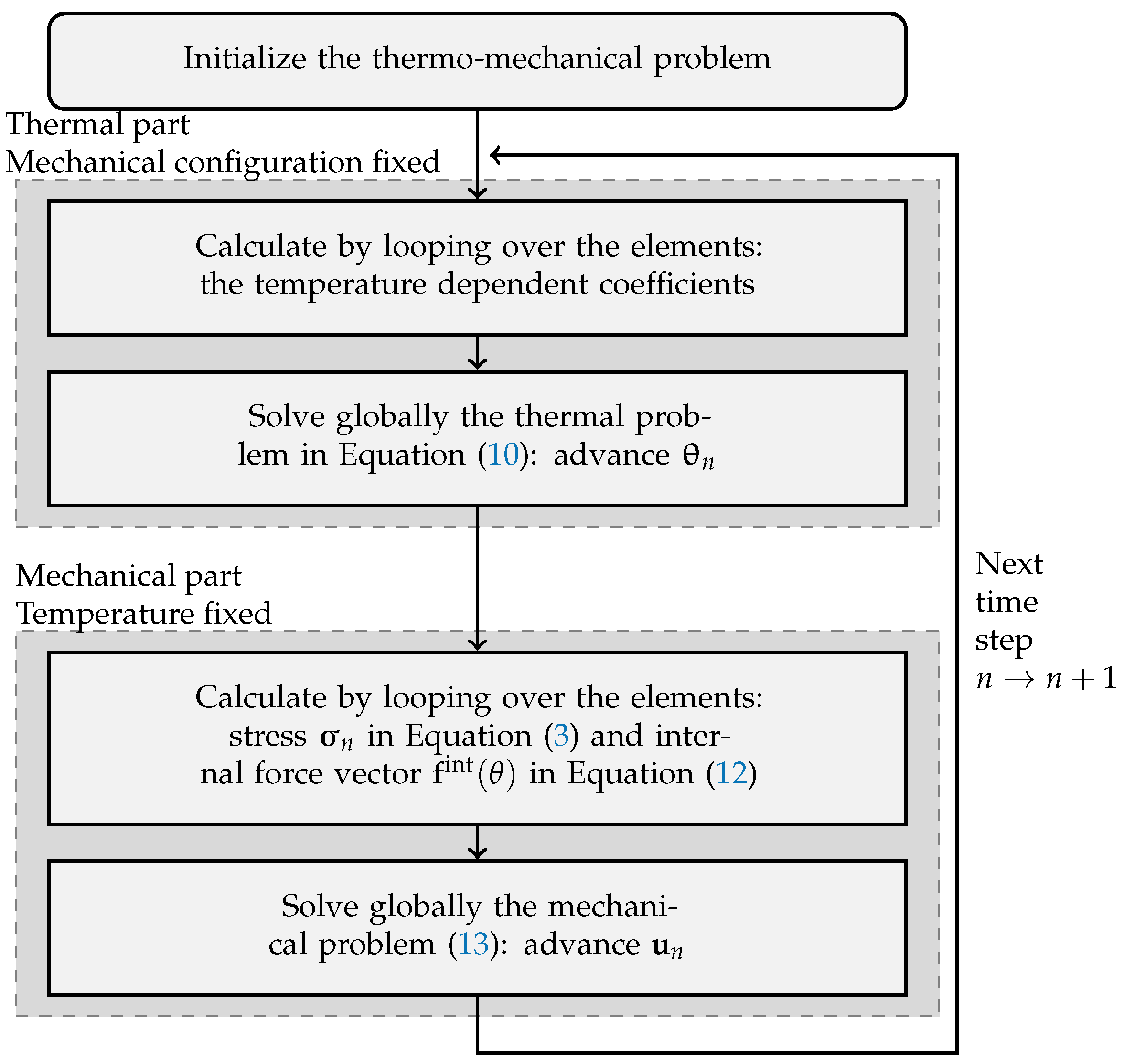
3.3. Solution Methods for the Global Thermo-Mechanical Problem
Explicit Scheme for the Uniaxial Compression Tests
4. Numerical Simulations: Results and Discussion
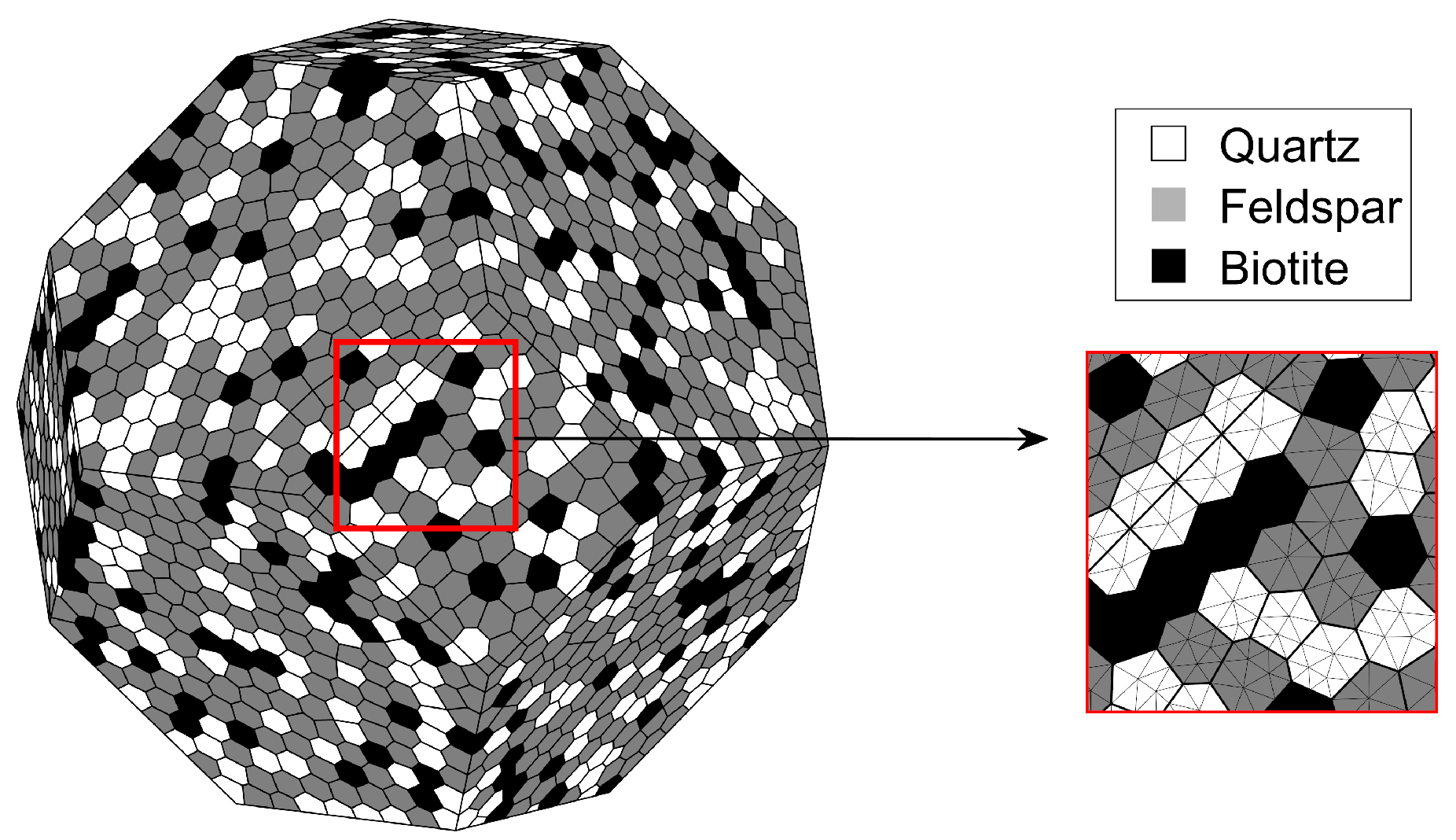
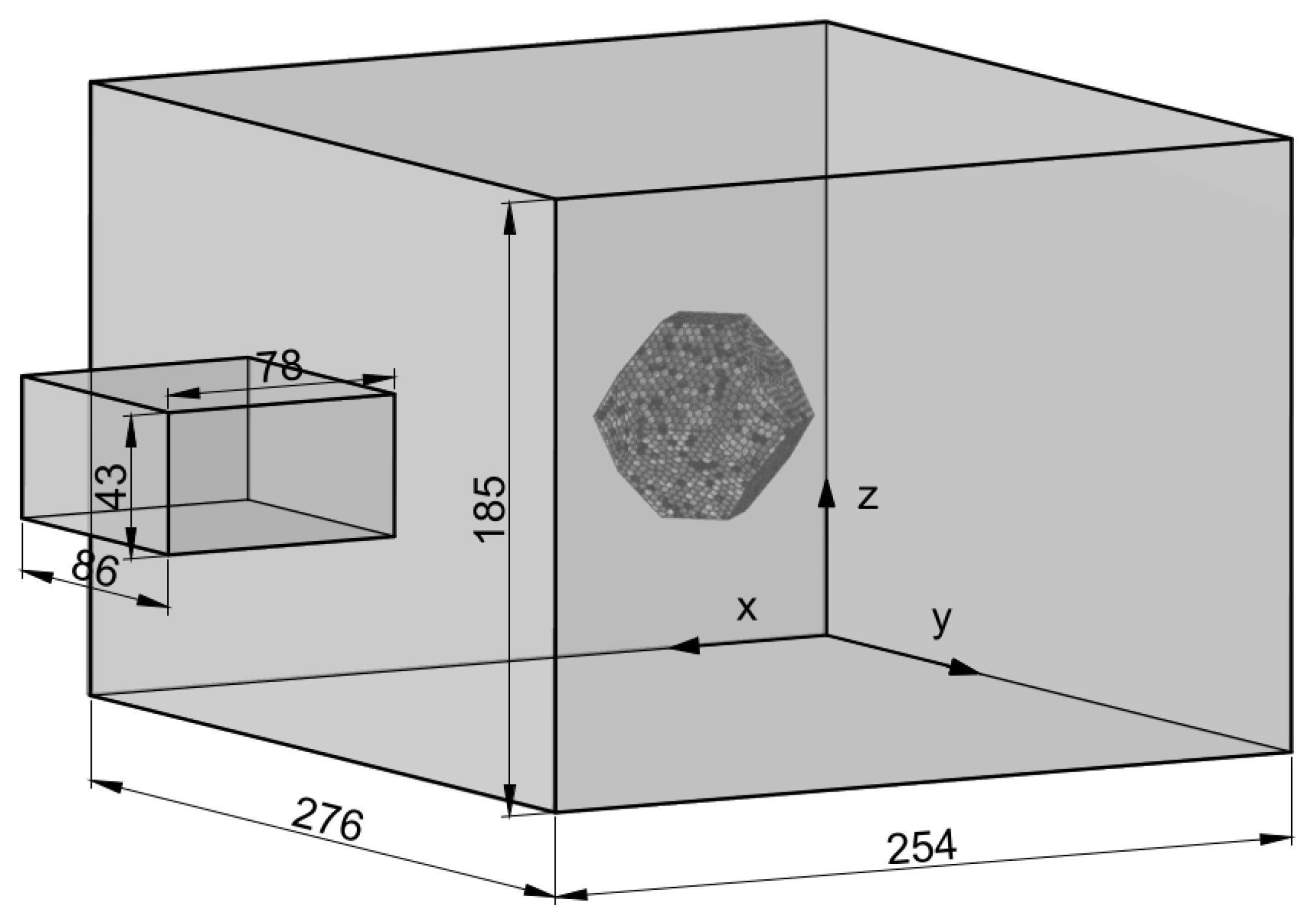
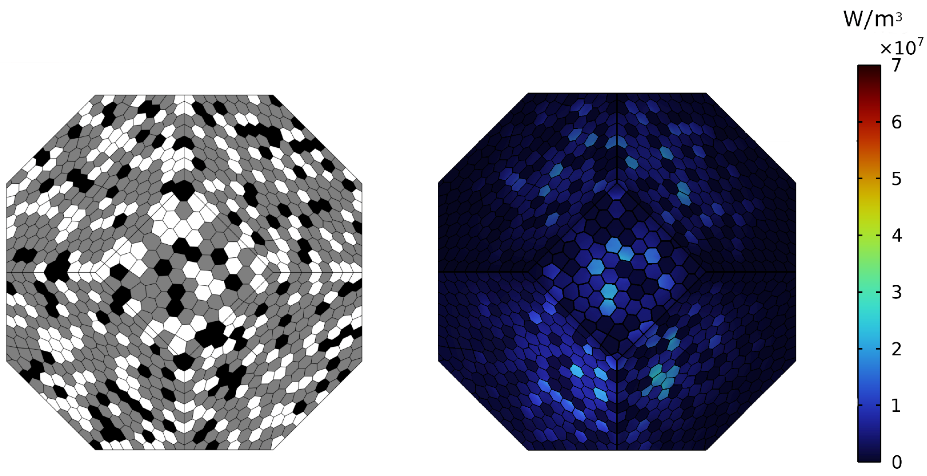
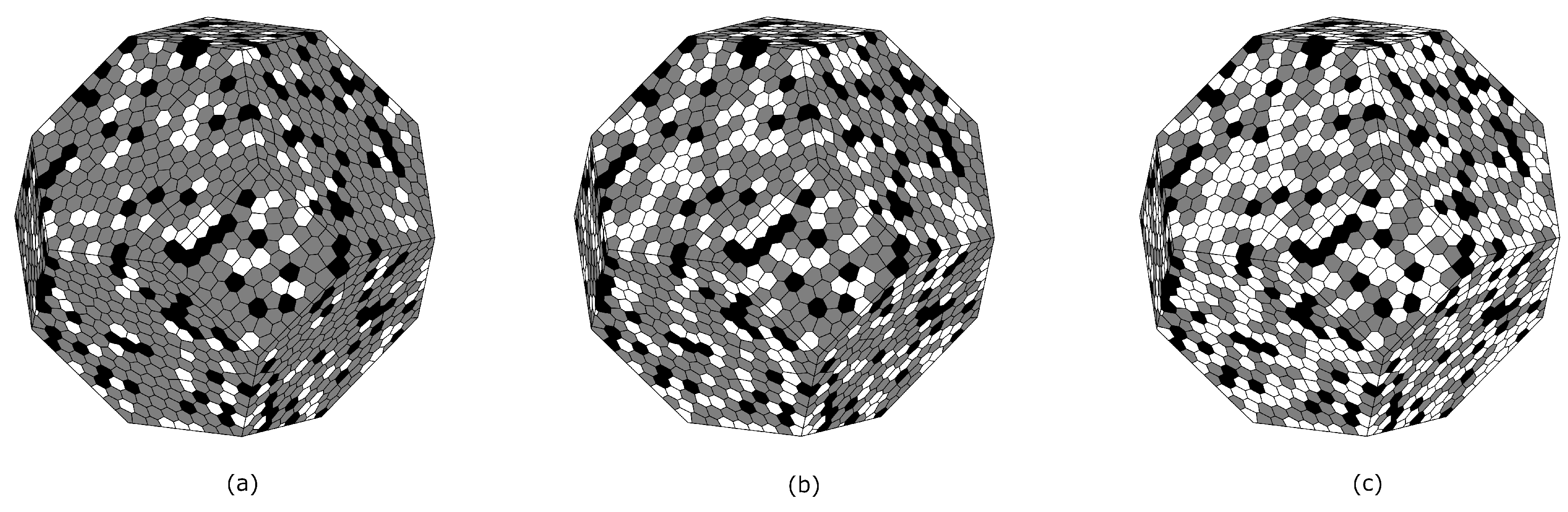
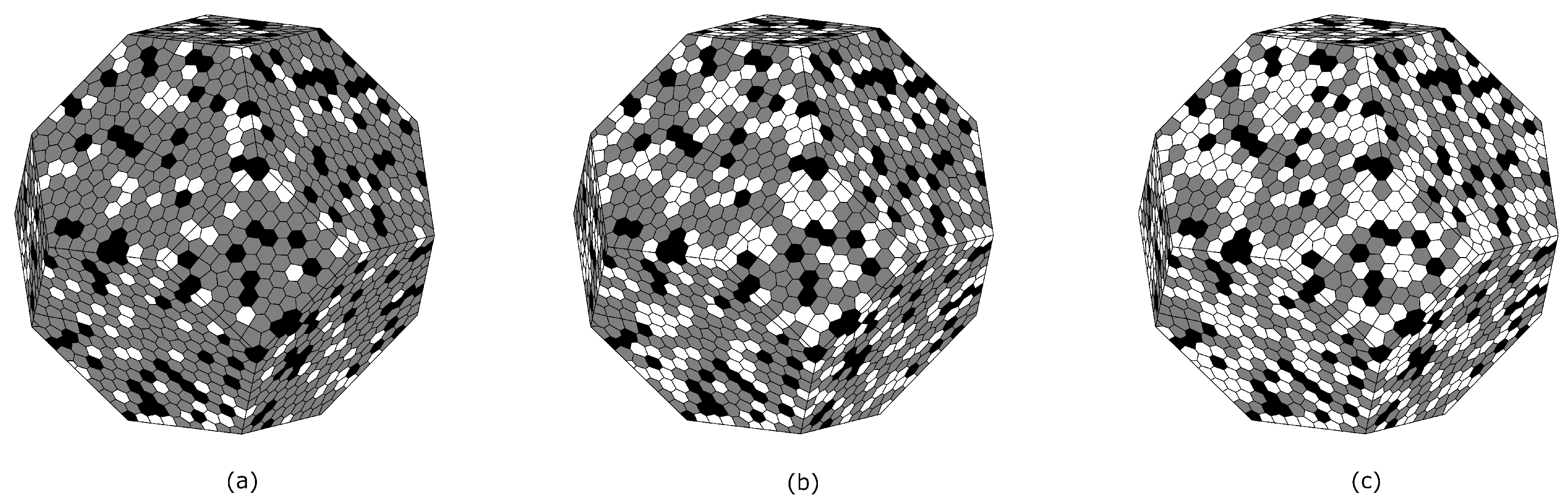
4.1. Material Heterogeneity and Mesostructure Description
4.2. Thermal Pretreatments on Numerical Rock Sample
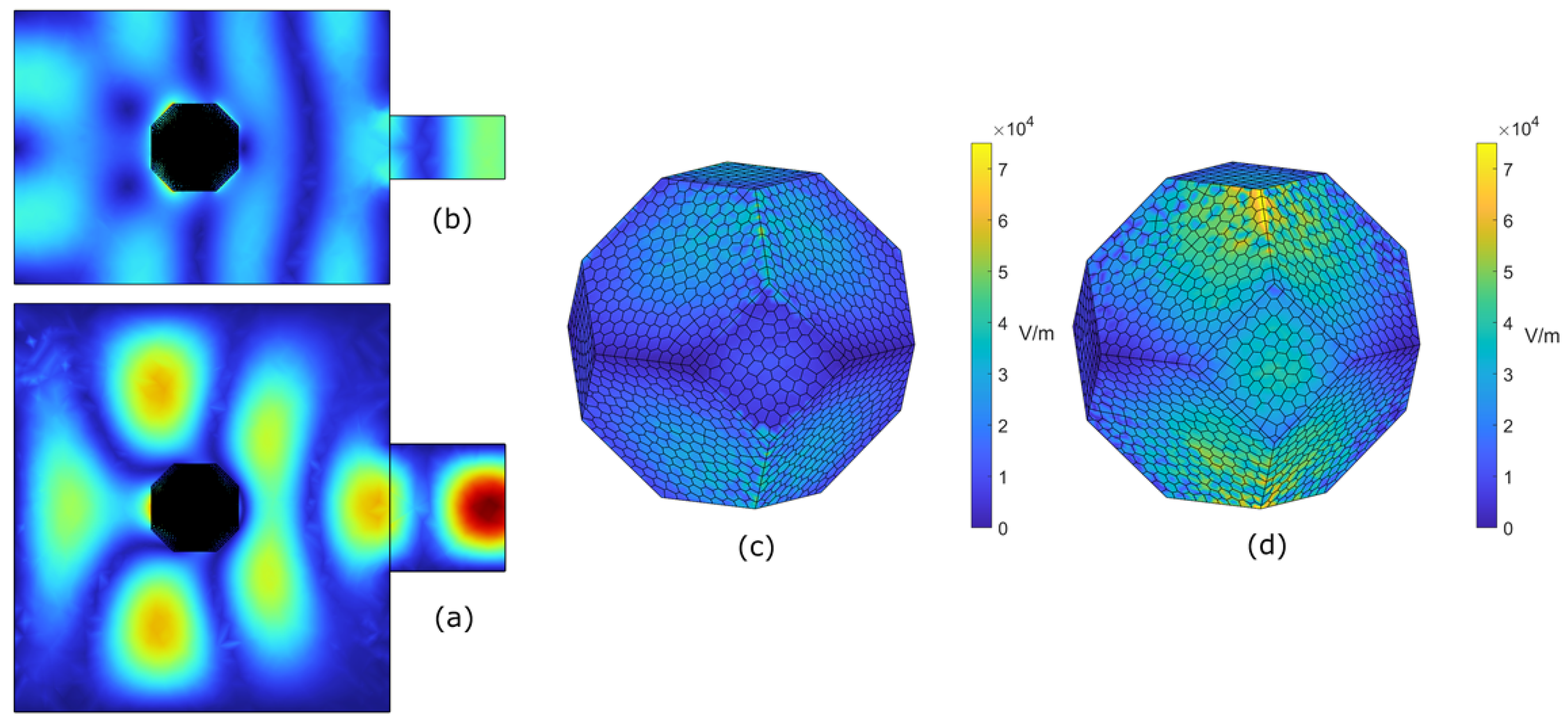
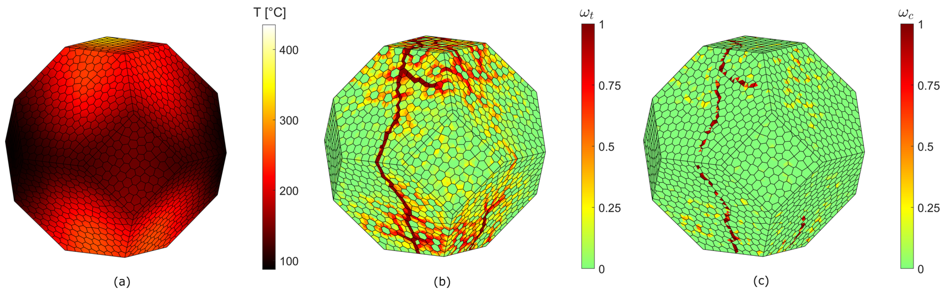
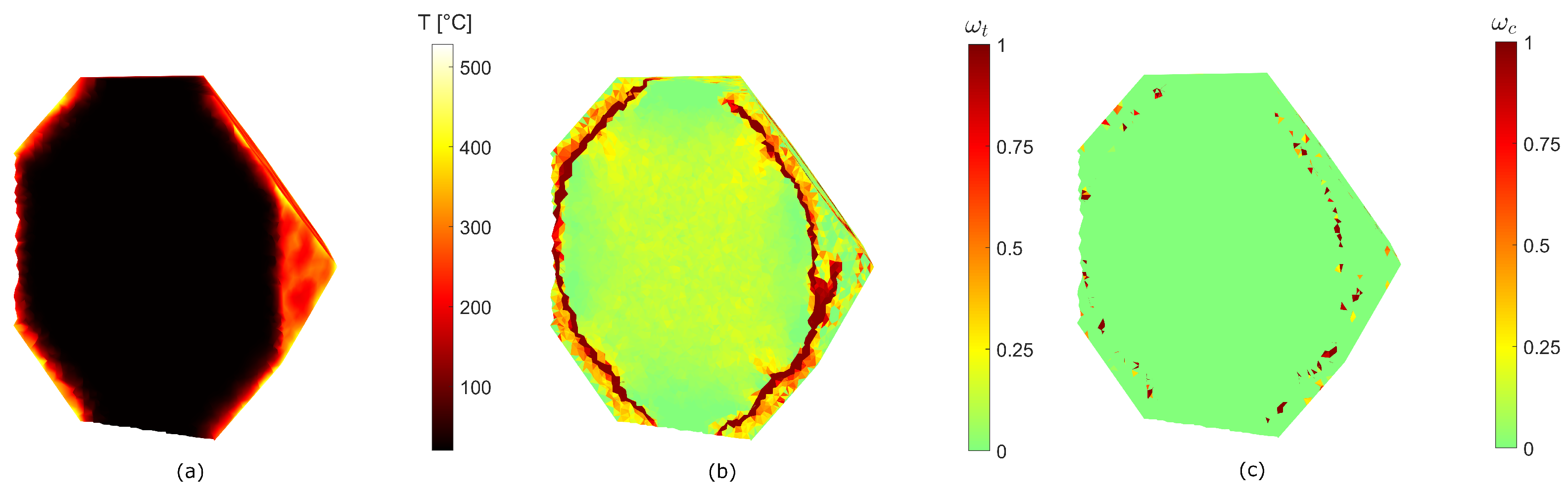
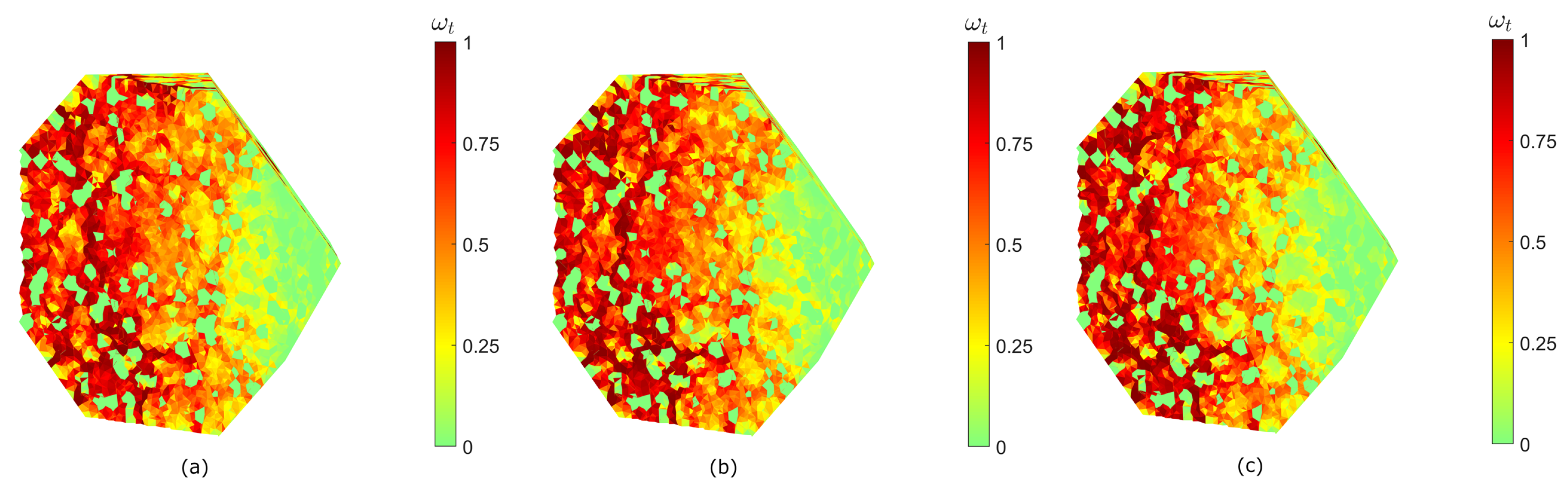
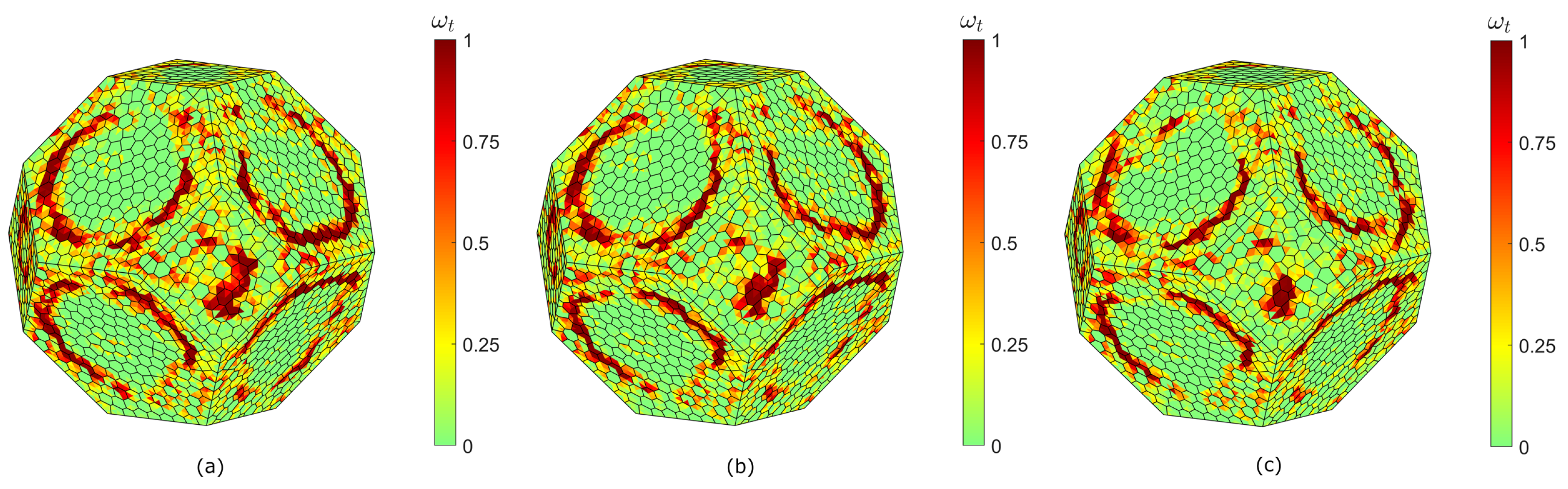
4.2.1. Microwave Pretreatment on Numerical Rock Sample
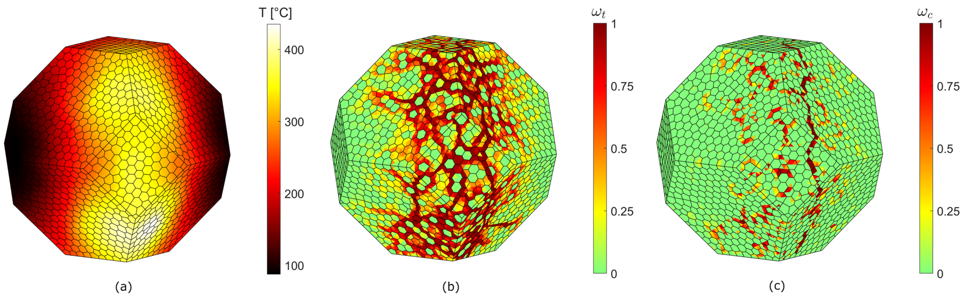
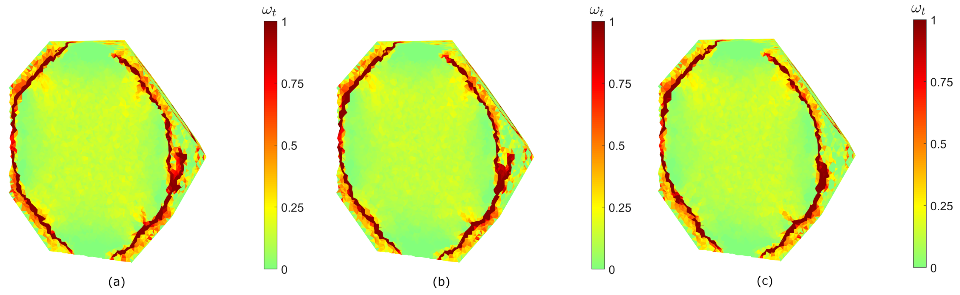
4.2.2. Conventional Heating Pretreatment on Numerical Rock Sample
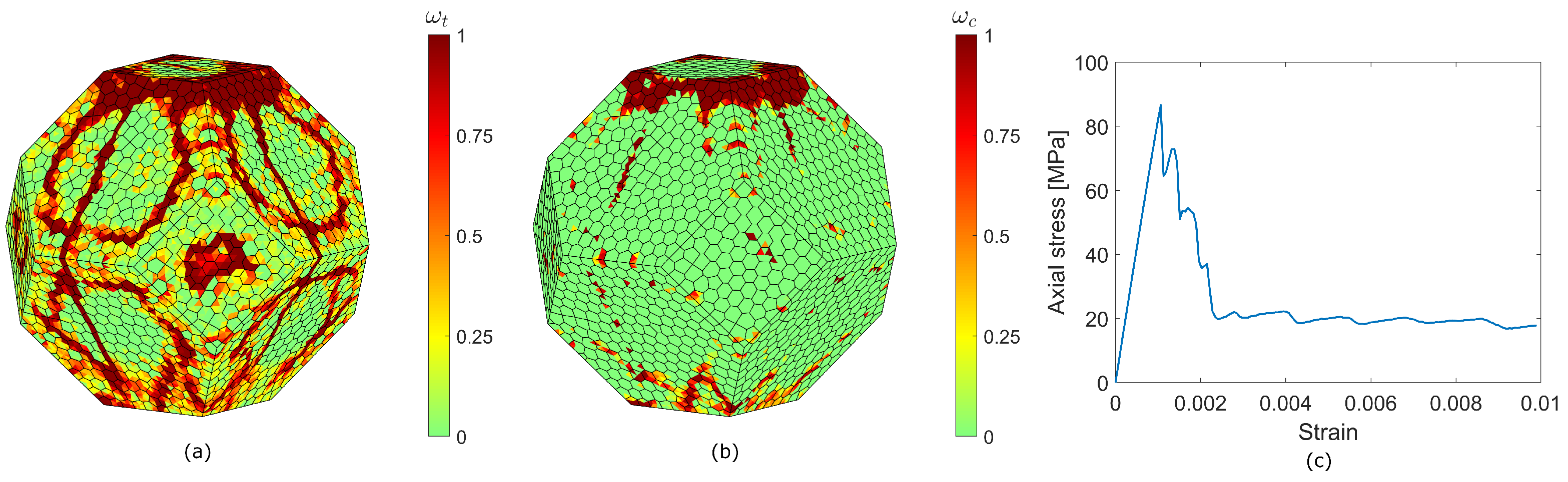
4.2.3. Influence of Quartz Content on Temperature and Tensile Damage Distribution during Thermal Pretreatment
- The geometry of tessellation is preserved;
- The original number and location of biotite grains are preserved;
- A certain number of quartz grains (original percentage 30%) replaces or is replaced by feldspar grains.
4.3. Uniaxial Compression Test on Numerical Rock Sample
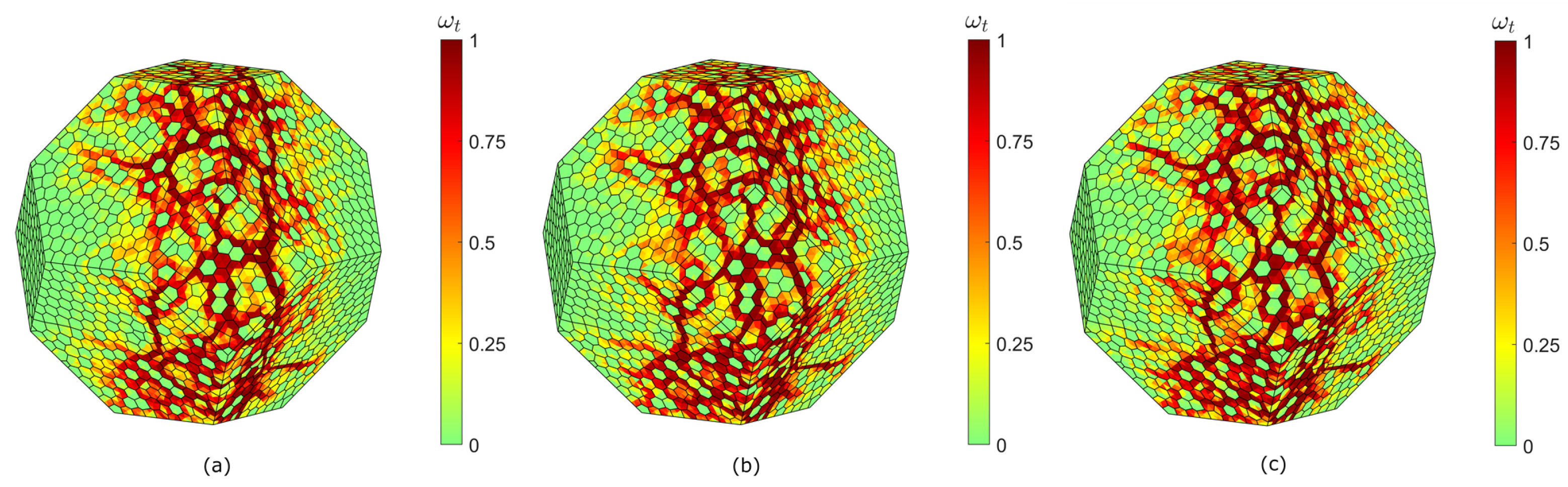
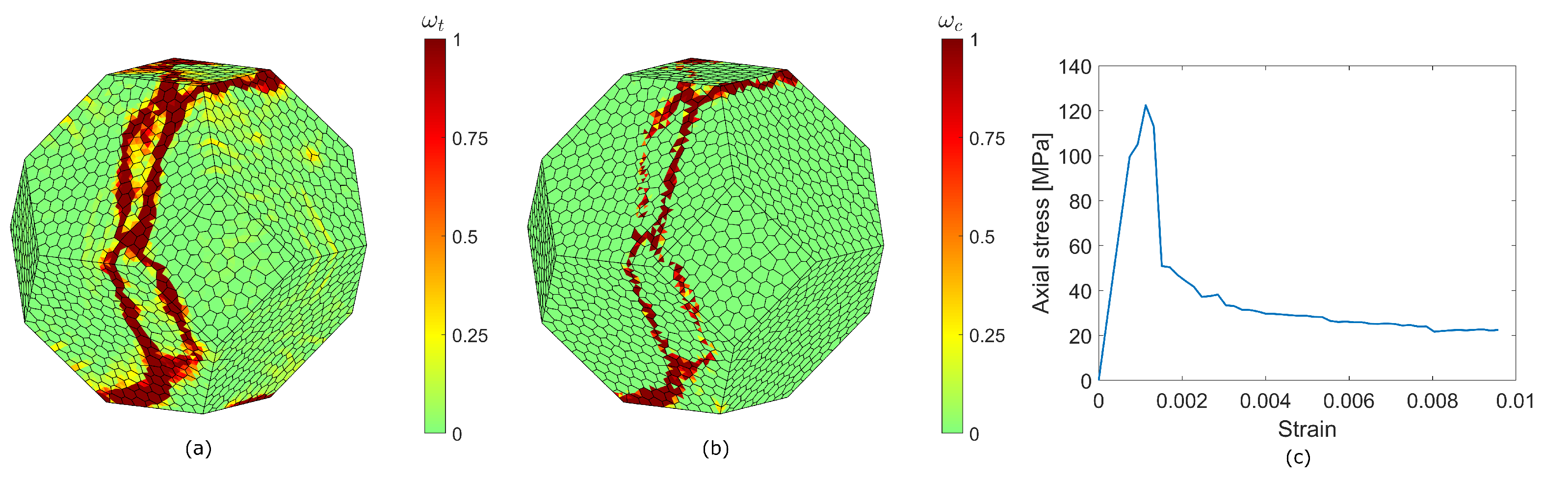
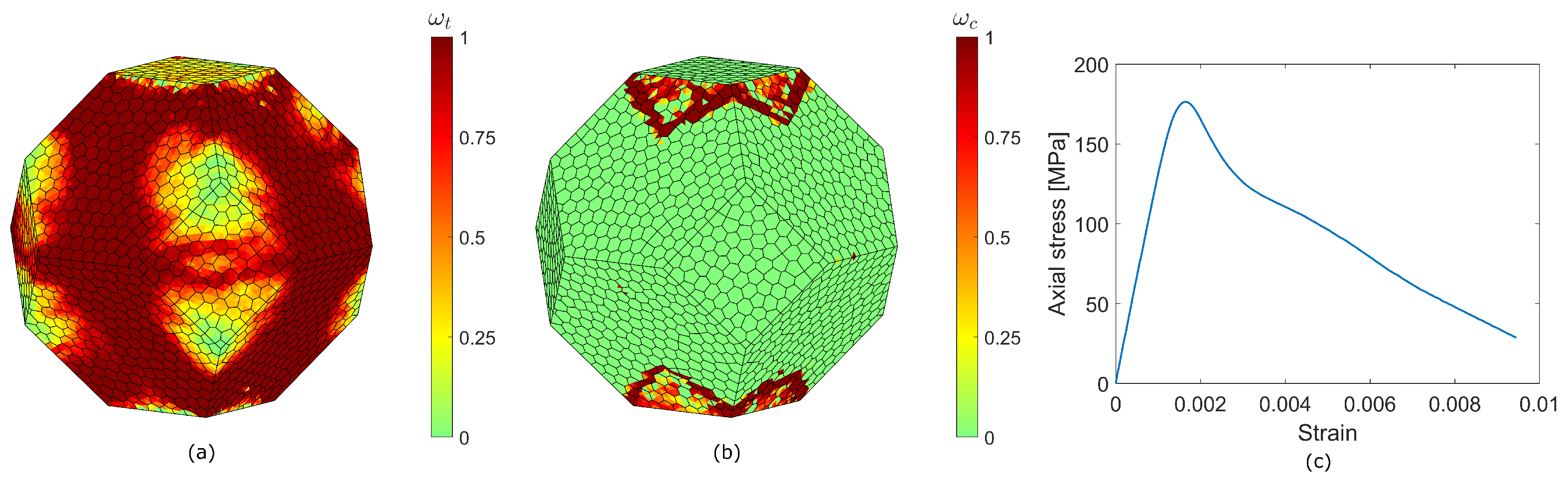
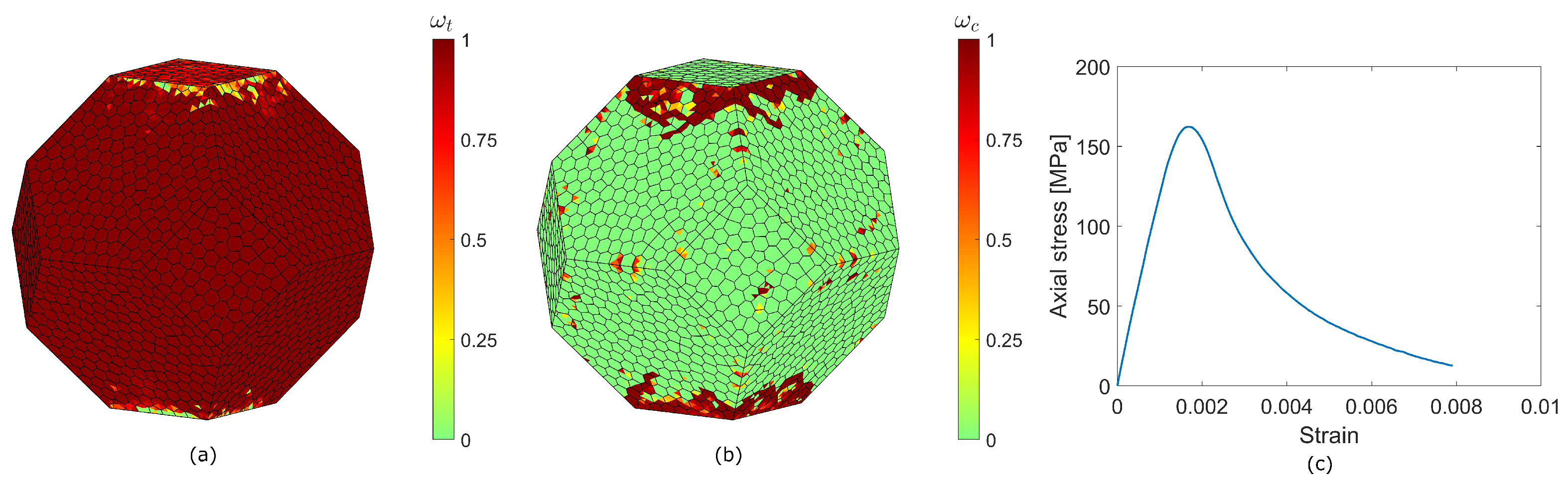
4.3.1. Uniaxial Compression Test on Intact Numerical Rock Sample
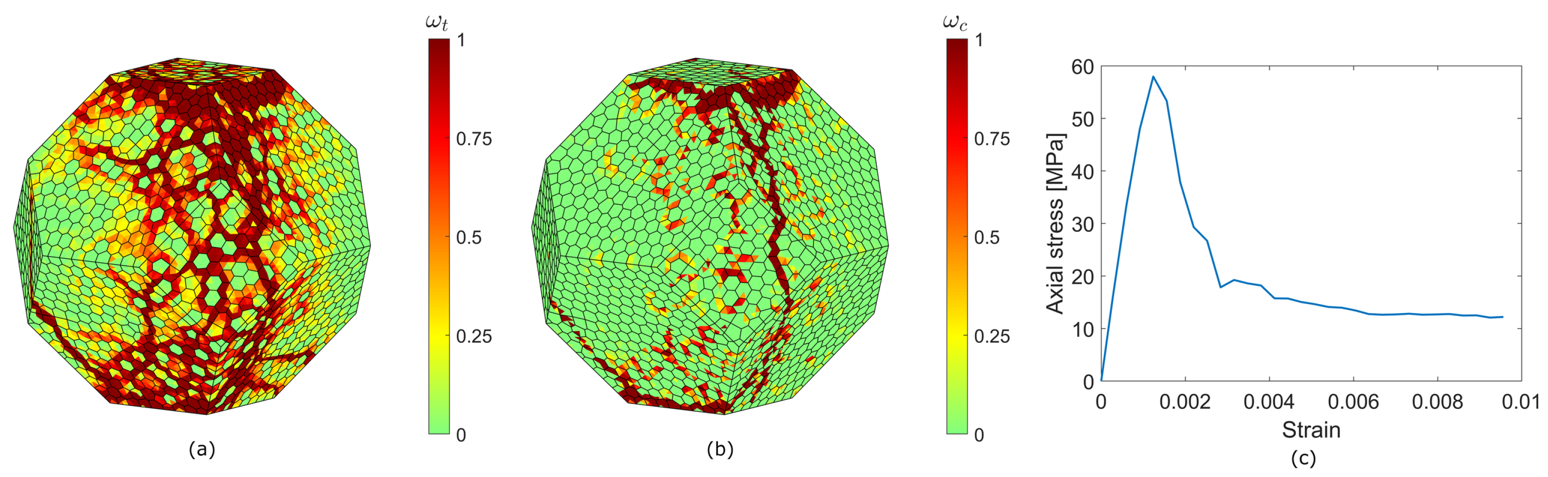
4.3.2. Uniaxial Compression Test on Numerical Rock Sample Pretreated with Microwave Irradiation
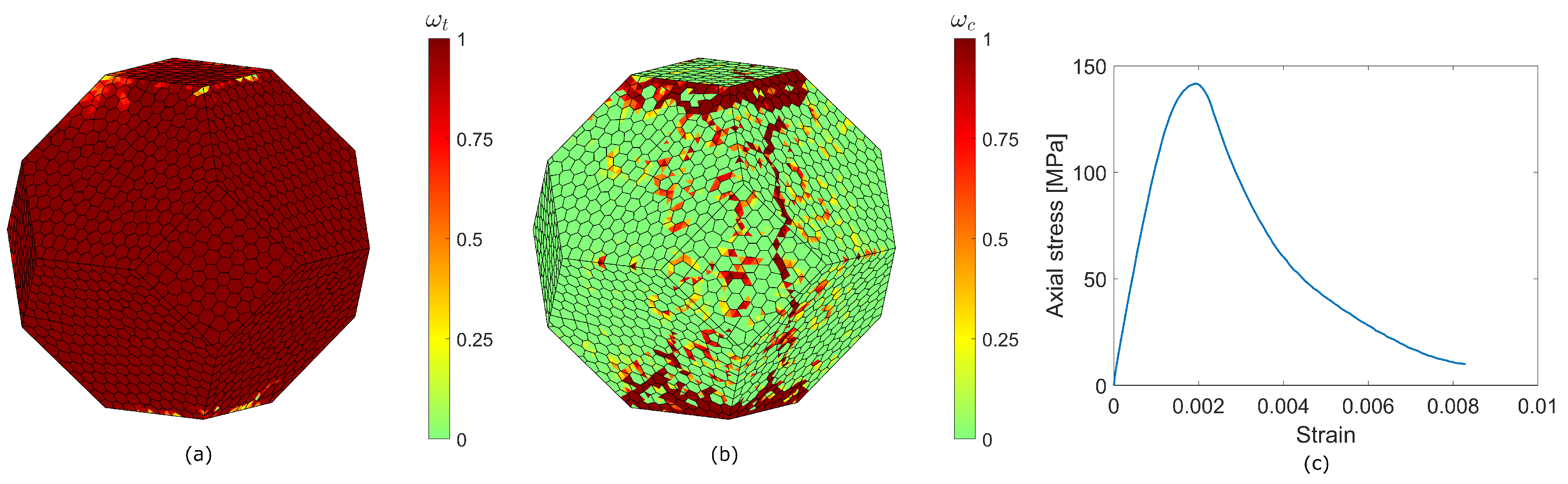
4.3.3. Uniaxial Compression Test on Numerical Rock Sample Pretreated with Conventional Heating
5. Discussion and Conclusions
- A method to simulate rock breakage due to thermal pretreatments (conventional heating and microwave irradiation), based on a continuum approach, is developed and tested in this paper. Rock failure is modelled via a damage-(visco)plasticity model derived from the Rankine and Drucker–Prager yield criteria. Stiffness degradation and strength deterioration are both taken into account by means of separate scalar damage parameters in tension and compression. Moreover, the unilateral conditions of tensile damage of rock are rendered through specific parameters that modelled the extreme cases of complete stiffness recovery or no stiffness recovery during load reversal from tension to compression.
- The adopted explicit staggered scheme proves to be effective in solving the nonlinear coupled problem of thermal cracking due to heating by microwave irradiation and conventional heating. Drastic mass scaling can be applied thanks to the non-inertial nature of the slow heating induced by both pretreatments. Mass scaling allows one to increase the critical time step of the explicit time marching scheme for the mechanical part of the governing global problem.
- Damage patterns are heavily influenced by the nature of the heating pretreatment (volumetric or surface) and by the heterogeneity of the material. Polycrystalline hard rocks such as granite are constituted of minerals with different dielectric, thermal and mechanical properties. Here, heterogeneity was defined explicitly by representing the typical granular texture of polycrystalline hard rock as a Voronoi structure of polyhedral cells. The advantage of this approach is evident especially in the microwave simulation results, where single biotite and quartz grains were entirely spared from damage due to their dielectric, thermal and mechanical properties.
- Conventional heating via heat torch, for these idealized and specific testing conditions, seems to be the best pretreatment in terms of highest ratio of uniaxial compressive strength reduction percentage to required energy seems to be the conventional heating method. However, it must be remarked that this method requires a very high surface heat flux (0.5 MW/m2) to reach the necessary temperature levels and ad hoc thermal equipment to obtain a uniform heating.
- On the other hand, microwave oven appliances are more commonly available, even though they demand longer heating times due to the low dielectric properties of granite. Moreover, the search for the best placement inside the cavity that maximizes the temperature outcomes can be time-consuming. Therefore, different time duration/heating power combinations should be tested in order to find the optimal ratio of strength reduction percentage vs. spent energy.
- The thermal pretreatment simulations are repeated for specimens having different quartz percentages. Two new specimens are created, one with 15% quartz content and the other with 45%. The number and location of biotite grains are preserved. Quartz grains are replaced by feldspar grains to obtain the desired quartz percentages. The results of microwave heating show a slight increase in average temperature with increasing quartz content. However, from the simulation results an immediate correlation between quartz content and tensile damage intensity cannot be established. The results of conventional heating may suggest an influence of quartz content on average temperature and tensile damage severity. In particular, average temperature and tensile damage seem to increase with decreasing quartz content.
- The simulation conditions are not ideal for comparison of these two thermal pretreatments, which are quite different in nature (surface heating vs. volumetric heating). The chosen approach here was to obtain similar temperature values in the samples. A more sound approach to estimate the efficacy of different thermal pretreatments is to compare not temperatures, but entering heat. In that case, the total energy spent during the 60 s microwave heating would be spread across the external heated surface (conventional heating). However, since the duration treatment in this case is quite short (to induce a sudden heat-shock in the sample), the external surface power and the temperatures reached in that case would have been high enough to cause melting in the sample. A solution could be to extend the duration of the conventional heating, but that would probably not produce the desired heat shock effect. Moreover, longer heating times imply lower feasibility and and practical application of the method in real-life mineral processing plant situations.
- Further developments of this study should include modelling of intergranular cracks at grain boundaries to replicate the experimental results of previous studies. Finally, in order to fully evaluate the weakening effect of thermal pretreatments on compressive strength of rock, the present model should be validated via laboratory experiments.
Author Contributions
Funding
Data Availability Statement
Conflicts of Interest
References
- Tromans, D. Mineral comminution: Energy efficiency considerations. Miner. Eng. 2008, 21, 613–620. [Google Scholar] [CrossRef]
- Musa, F.; Morrison, R. A more sustainable approach to assessing comminution efficiency. Miner. Eng. 2009, 22, 593–601. [Google Scholar] [CrossRef]
- Ballantyne, G.; Powell, M. Benchmarking comminution energy consumption for the processing of copper and gold ores. Miner. Eng. 2014, 65, 109–114. [Google Scholar] [CrossRef]
- Curry, J.A.; Ismay, M.J.; Jameson, G.J. Mine operating costs and the potential impacts of energy and grinding. Miner. Eng. 2014, 56, 70–80. [Google Scholar] [CrossRef]
- Napier-Munn, T. Is progress in energy-efficient comminution doomed? Miner. Eng. 2015, 73, 1–6. [Google Scholar] [CrossRef]
- Klein, B.; Wang, C.; Nadolski, S. Energy-Efficient Comminution: Best Practices and Future Research Needs. In Energy Efficiency in the Minerals Industry: Best Practices and Research Directions; Awuah-Offei, K., Ed.; Springer International Publishing: Cham, Switzerland, 2018; pp. 197–211. [Google Scholar]
- Tutak, M.; Brodny, J. Forecasting Methane Emissions from Hard Coal Mines Including the Methane Drainage Process. Energies 2019, 12, 3840. [Google Scholar] [CrossRef]
- Somani, A.; Nandi, T.K.; Pal, S.K.; Majumder, A.K. Pre-treatment of rocks prior to comminution—A critical review of present practices. Int. J. Min. Sci. Technol. 2017, 27, 339–348. [Google Scholar] [CrossRef]
- Fitzgibbon, K.; Veasey, T. Thermally assisted liberation—A review. Miner. Eng. 1990, 3, 181–185. [Google Scholar] [CrossRef]
- Wang, Y.; Wang, Z.; Shi, L.; Rong, Y.; Hu, J.; Jiang, G.; Wang, Y.; Hu, S. Anisotropic Differences in the Thermal Conductivity of Rocks: A Summary from Core Measurement Data in East China. Minerals 2021, 11, 1135. [Google Scholar] [CrossRef]
- Somerton, W. Thermal Properties and Temperature-Related Behavior of Rock/Fluid Systems; Elsevier Science: Amsterdam, The Netherlands, 1992. [Google Scholar]
- Wu, X.; Huang, Z.; Song, H. Variations of Physical and Mechanical Properties of Heated Granite After Rapid Cooling with Liquid Nitrogen. Rock Mech. Rock Eng. 2019, 52, 2123–2139. [Google Scholar] [CrossRef]
- Forster, J. Dielectric Properties of Minerals and Ores and the Application of Microwaves for Assisted Comminution. Ph.D. Thesis, University of Toronto, Toronto, ON, Canada, 2023. [Google Scholar]
- Teimoori, K.; Hassani, F. Twenty years of experimental and numerical studies on microwave-assisted breakage of rocks and minerals—A review. arXiv 2020, arXiv:2011.14624. [Google Scholar]
- Jones, D.; Lelyveld, T.; Mavrofidis, S.; Kingman, S.; Miles, N. Microwave heating applications in environmental engineering—A review. Resour. Conserv. Recycl. 2002, 34, 75–90. [Google Scholar] [CrossRef]
- Monti, T.; Tselev, A.; Udoudo, O.; Ivanov, I.; Dodds, C.; Kingman, S. High-resolution dielectric characterization of minerals: A step towards understanding the basic interactions between microwaves and rocks. Int. J. Miner. Process. 2016, 151, 8–21. [Google Scholar] [CrossRef]
- Palma, V.; Barba, D.; Cortese, M.; Martino, M.; Renda, S.; Meloni, E. Microwaves and Heterogeneous Catalysis: A Review on Selected Catalytic Processes. Catalysts 2020, 10, 246. [Google Scholar] [CrossRef]
- Tian, W.; Yang, S.; Huang, Y.; Hu, B. Mechanical Behavior of Granite with Different Grain Sizes After High-Temperature Treatment by Particle Flow Simulation. Rock Mech. Rock Eng. 2020, 53, 1791–1807. [Google Scholar] [CrossRef]
- Saksala, T. Numerical Modeling of Temperature Effect on Tensile Strength of Granitic Rock. Appl. Sci. 2021, 11, 4407. [Google Scholar] [CrossRef]
- Ma, Z.; Zheng, Y.; Sun, T.; Li, J. Thermal stresses and temperature distribution of granite under microwave treatment. In Proceedings of the 11th Conference of Asian Rock Mechanics Society, Bristol, UK, 21–25 October 2021; Volume 861. [Google Scholar]
- Zhu, J.; Yi, L.; Yang, Z.; Duan, M. Three-dimensional numerical simulation on the thermal response of oil shale subjected to microwave heating. Chem. Eng. J. 2021, 407, 127197. [Google Scholar] [CrossRef]
- Toifl, M.; Meisels, R.; Hartlieb, P.; Kuchar, F.; Antretter, T. 3D numerical study on microwave induced stresses in inhomogeneous hard rocks. Miner. Eng. 2016, 90, 29–42. [Google Scholar] [CrossRef]
- Xu, T.; Yuan, Y.; Heap, M.J.; Zhou, G.L.; Perera, M.; Ranjith, P. Microwave-assisted damage and fracturing of hard rocks and its implications for effective mineral resources recovery. Miner. Eng. 2021, 160, 106663. [Google Scholar] [CrossRef]
- Wei, W.; Shao, Z.; Zhang, P.; Zhang, H.; Cheng, J.; Yuan, Y. Thermally Assisted Liberation of Concrete and Aggregate Recycling: Comparison between Microwave and Conventional Heating. J. Mater. Civ. Eng. 2021, 33, 04021370. [Google Scholar] [CrossRef]
- Shou, H.Z.; Hu, Q.; Zeng, J.; He, L.; Tang, H.; Li, B.; Chen, S.; Lu, X. Comparative study on the deterioration of granite under microwave irradiation and resistance-heating treatment. Frat. Ed Integrità Strutt. 2019, 13, 638–648. [Google Scholar] [CrossRef]
- Pressacco, M.; Kangas, J.; Saksala, T. Numerical Modelling of Microwave Heating Assisted Rock Fracture. Rock Mech. Rock Eng. 2022, 55, 481–503. [Google Scholar] [CrossRef]
- Saksala, T. Damage–viscoplastic consistency model with a parabolic cap for rocks with brittle and ductile behavior under low-velocity impact loading. Int. J. Numer. Anal. Meth. 2010, 34, 1362–1386. [Google Scholar] [CrossRef]
- Wang, W.M. Stationary and Propagative Instabilities in Metals—A Computational Point of View. Ph.D. Thesis, Delft University of Technology, Delft, The Netherlands, 1997. [Google Scholar]
- Wang, W.M.; Sluys, L.J.; de Borst, R. Viscoplasticity for instabilities due to strain softening and strain-rate softening. Int. J. Numer. Meth. Eng. 1997, 40, 3839–3864. [Google Scholar] [CrossRef]
- Grassl, P.; Jirásek, M. Damage-plastic model for concrete failure. Int. J. Solids Struct. 2006, 43, 7166–7196. [Google Scholar] [CrossRef]
- Lubliner, J.; Oliver, J.; Oñate, E. A plastic-damage model for concrete. Int. J. Solids Struct. 1989, 25, 299–326. [Google Scholar] [CrossRef]
- Lee, J.; Fenves, G.L. Plastic-Damage Model for Cyclic Loading of Concrete Structures. J. Eng. Mech. 1998, 124, 892–900. [Google Scholar] [CrossRef]
- Eberhardt, E.; Stead, D.; Stimpson, B. Quantifying progressive pre-peak brittle fracture damage in rock during uniaxial compression. Int. J. Rock Mech. Min. 1999, 36, 361–380. [Google Scholar] [CrossRef]
- Wang, H.; Rezaee, M.; Saeedi, A.; Josh, M. Numerical modelling of microwave heating treatment for tight gas sand reservoirs. J. Pet. Sci. Eng. 2017, 152, 495–504. [Google Scholar] [CrossRef]
- Ottosen, N.S.; Ristinmaa, M. The Mechanics of Constitutive Modeling; Elsevier Science Ltd.: Oxford, UK, 2005; pp. 637–672. [Google Scholar]
- Poole, C.; Darwazeh, I. Microwave Active Circuit Analysis and Design; Academic Press: Oxford, UK, 2016. [Google Scholar]
- Monk, P. Finite Element Methods for Maxwell’s Equations; Oxford University Press: Oxford, UK, 2003. [Google Scholar]
- Pozar, D.M. Microwave Engineering; Wiley: Hoboken, NJ, USA, 2011. [Google Scholar]
- Haus, H.A.; Melcher, J.R. Electromagnetic Fields and Energy; Prentice-Hall: Englewood Cliffs, NJ, USA, 1989. [Google Scholar]
- Jackson, J.D. Classical Electrodynamics; John Wiley & Sons: New York, NY, USA, 1998. [Google Scholar]
- Pressacco, M.; Saksala, T. Numerical modelling of heat shock-assisted rock fracture. Int. Numer. Anal. Meth. Geomech. 2020, 44, 40–68. [Google Scholar] [CrossRef]
- Ngo, M.; Brancherie, D.; Ibrahimbegovic, A. Softening behavior of quasi-brittle material under full thermo-mechanical coupling condition: Theoretical formulation and finite element implementation. Comput. Methods Appl. Mech. Eng. 2014, 281, 1–28. [Google Scholar] [CrossRef]
- Felippa, C.A.; Park, C.K. Staggered transient analysis procedures for coupled mechanical systems: Formulation. Comput. Methods Appl. Mech. Eng. 1980, 24, 61–111. [Google Scholar] [CrossRef]
- Martins, J.M.P.; Neto, D.M.; Alves, J.L.; Oliveira, M.C.; Laurent, H.; Andrade-Campos, A.; Menezes, L.F. A new staggered algorithm for thermomechanical coupled problems. Int. J. Solids Struct. 2017, 122–123, 42–58. [Google Scholar] [CrossRef]
- Hahn, G.D. A modified Euler method for dynamic analyses. Int. J. Numer. Meth. Eng. 1991, 32, 943–955. [Google Scholar] [CrossRef]
- Quey, R.; Dawson, P.; Barbe, F. Large-scale 3D random polycrystals for the finite element method: Generation, meshing and remeshing. Comput. Methods Appl. Mech. Eng. 2011, 200, 1729–1745. [Google Scholar] [CrossRef]
- Vázquez, P.; Shushakova, V.; Gómez-Heras, M. Influence of mineralogy on granite decay induced by temperature increase: Experimental observations and stress simulation. Eng. Geol. 2015, 189, 58–67. [Google Scholar] [CrossRef]
- Zheng, Y.L.; Zhao, X.B.; Zhao, Q.H.; Li, J.C.; Zhang, Q.B. Dielectric properties of hard rock minerals and implications for microwave-assisted rock fracturing. Geomech. Geophys. Geo-Energy Geo-Resour. 2020, 6, 97–122. [Google Scholar] [CrossRef]
- Mahabadi, O.K. Investigating the Influence of Micro-scale Heterogeneity and Microstructure on the Failure and Mechanical Behaviour of Geomaterials. Ph.D. Thesis, University of Toronto, Toronto, ON, Canada, 2012. [Google Scholar]
- Schön, J. Physical Properties of Rocks; Elsevier Science and Technology: London, UK, 2011; p. 494. [Google Scholar]
- Clauser, C.; Huenges, E. Thermal Conductivity of Rocks and Minerals. In Rock Physics & Phase Relations; American Geophysical Union (AGU): Washington, DC, USA, 2013; pp. 105–126. [Google Scholar]
- Waples, D.W.; Waples, J.S. A Review and Evaluation of Specific Heat Capacities of Rocks, Minerals and Subsurface Fluids. Part 1: Minerals and Nonporous Rocks. Nat. Resour. Res. 2004, 13, 97–122. [Google Scholar] [CrossRef]
- Park, J.W.; Park, C.; Ryu, D.; Park, E.S. Numerical simulation of thermo-mechanical behavior of rock using a grain-based distinct element model. In ISRM Regional Symposium-EUROCK; Austrian Society for Geomechanics: Salzburg, Austria, 2015. [Google Scholar]
- Saksala, T. 3D Numerical Prediction of Thermal Weakening of Granite under Tension. Geosciences 2022, 12, 10. [Google Scholar] [CrossRef]
- Wang, F.; Konietzky, H. Thermo-Mechanical Properties of Granite at Elevated Temperatures and Numerical Simulation of Thermal Cracking. Rock Mech. Rock Eng. 2019, 52, 3737–3755. [Google Scholar] [CrossRef]
- Santos, T.C.; Costa, L.C.; Valente, M.A.; Monteiro, J.; Sousa, J.; Santos, T. 3D Electromagnetic Field Simulation in Microwave Ovens: A Tool to Control Thermal Runaway. In Proceedings of the COMSOL Conference, Newton, MA, USA, 7–9 October 2010. [Google Scholar]
- Teimoori, K.; Cooper, R. Multiphysics study of microwave irradiation effects on rock breakage system. Int. J. Rock Mech. Min. Sci. 2021, 140, 104586. [Google Scholar] [CrossRef]
- Roshankhah, S.; Teimoori, K.; Mohammadi, K. Thermo-Mechanical Response of Layered Rocks upon Single-Mode Microwave Treatments. In Proceedings of the ARMA/DGS/SEG International Geomechanics Symposium, Virtual, 1–4 November 2021. [Google Scholar]
- Shadi, A.; Ahmadihosseini, A.; Rabiei, M.; Samea, P.; Hassani, F.; Sasmito, A.P.; Ghoreishi-Madiseh, S.A. Numerical and experimental analysis of fully coupled electromagnetic and thermal phenomena in microwave heating of rocks. Miner. Eng. 2022, 178, 107406. [Google Scholar] [CrossRef]
- Molaro, J.L.; Byrne, S.; Langer, S.A. Grain-scale thermoelastic stresses and spatiotemporal temperature gradients on airless bodies, implications for rock breakdown. J. Geophys. Res. Planet 2015, 120, 255–277. [Google Scholar] [CrossRef]
- Ge, Z.; Sun, Q.; Xue, L.; Yang, T. The influence of microwave treatment on the mode I fracture toughness of granite. Eng. Fract. Mech. 2021, 249, 107768. [Google Scholar] [CrossRef]
- Basu, A.; Mishra, D.; Roychowdhury, K. Rock failure modes under uniaxial compression, Brazilian and point load tests. Bull. Eng. Geol. Environ. 2013, 72, 457–475. [Google Scholar] [CrossRef]


| Parameter | Quartz | Feldspar | Biotite | ||
|---|---|---|---|---|---|
| Percentage in the sample | (%) | 30 | 55 | 15 | |
| [50] | (Density) | (/) | 2650 | 2620 | 3050 |
| E [49] | (Elastic modulus) | () | 80 | 60 | 20 |
| [49] | (Poisson’s ratio) | 0.17 | 0.29 | 0.20 | |
| [49] | (Tensile strength) | () | 10 | 8 | 7 |
| c | (Cohesion) | () | 25 | 25 | 25 |
| [49] | (Internal friction angle) | (°) | 50 | 50 | 50 |
| [49] | (Mode I fracture energy) | (/) | 40 | 40 | 28 |
| (Mode II fracture energy) | (/) | ||||
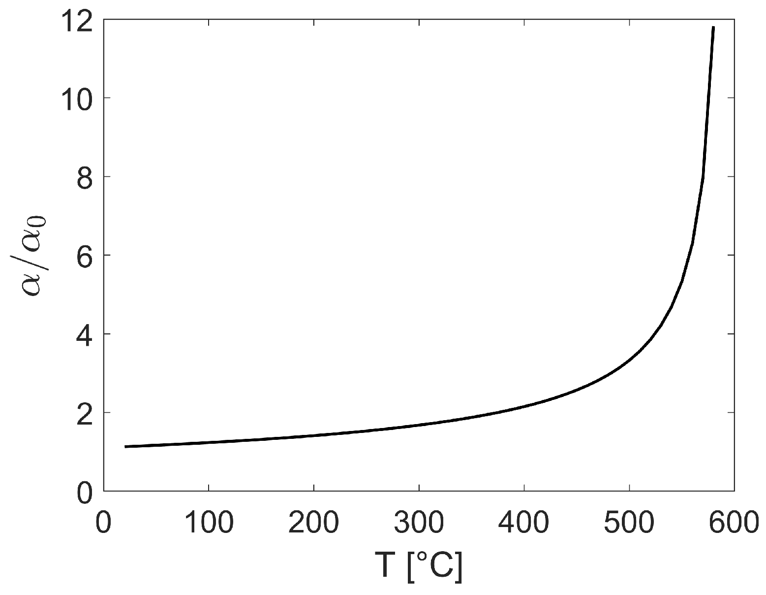
| [53] | (Thermal expansion coefficient) | (1/) | |||
| k [51] | (Thermal conductivity) | (/) | 4.94 | 2.34 | 3.14 |
| [52] | (Specific heat capacity) | (/) | 731 | 730 | 770 |
| [48] | (Dielectric constant) | 4.72 | 5.55 | 7.48 | |
| [48] | (Loss factor) | 0.014 | 0.118 | 0.456 | |
Disclaimer/Publisher’s Note: The statements, opinions and data contained in all publications are solely those of the individual author(s) and contributor(s) and not of MDPI and/or the editor(s). MDPI and/or the editor(s) disclaim responsibility for any injury to people or property resulting from any ideas, methods, instructions or products referred to in the content. |
© 2023 by the authors. Licensee MDPI, Basel, Switzerland. This article is an open access article distributed under the terms and conditions of the Creative Commons Attribution (CC BY) license (https://creativecommons.org/licenses/by/4.0/).
Share and Cite
Pressacco, M.; Kangas, J.; Saksala, T. Comparative Numerical Study on the Weakening Effects of Microwave Irradiation and Surface Flux Heating Pretreatments in Comminution of Granite. Geosciences 2023, 13, 132. https://doi.org/10.3390/geosciences13050132
Pressacco M, Kangas J, Saksala T. Comparative Numerical Study on the Weakening Effects of Microwave Irradiation and Surface Flux Heating Pretreatments in Comminution of Granite. Geosciences. 2023; 13(5):132. https://doi.org/10.3390/geosciences13050132
Chicago/Turabian StylePressacco, Martina, Jari Kangas, and Timo Saksala. 2023. "Comparative Numerical Study on the Weakening Effects of Microwave Irradiation and Surface Flux Heating Pretreatments in Comminution of Granite" Geosciences 13, no. 5: 132. https://doi.org/10.3390/geosciences13050132