Article

Understanding the Spatial Variability of the Relationship between InSAR-Derived Deformation and Groundwater Level Using Machine Learning

1
CSIRO Environment, Floreat, WA 6014, Australia
2
CSIRO Environment, Urrbrae, SA 5064, Australia
*
Author to whom correspondence should be addressed.
Geosciences 2023, 13(5), 133; https://doi.org/10.3390/geosciences13050133
Submission received: 11 March 2023 / Revised: 28 April 2023 / Accepted: 2 May 2023 / Published: 4 May 2023
(This article belongs to the Section Hydrogeology)

Abstract

:
The interferometric synthetic aperture radar (InSAR) technique was used in this study to derive the temporal and spatial information of ground deformation and explore its temporal correlation with groundwater dynamics. The random forest (RF) machine learning method was used to model the spatial variability of the temporal correlation and understand its influential contributors. The results showed that groundwater dynamics appeared to be an important factor in InSAR deformation at some bores where strong and positive correlations were observed. The RF model could explain up to 72% of spatial variances between InSAR deformation and groundwater dynamics. The spatial and temporal InSAR coherence (a proxy for the noise in InSAR results that is strongly related to vegetation) and soil moisture (difference, trend, and amplitude) were the most important factors explaining the spatial pattern of the temporal correlation between InSAR displacements and groundwater levels. This result confirms that noise sources (including deformation model fitting errors and radar signal decorrelation) and perturbation of the InSAR signal related to vegetation and surficial soils (clay content, moisture changes) should be accounted for when interpreting InSAR to support groundwater-related risk assessments and in groundwater resource management activities.

1. Introduction

Land subsidence, which includes both gentle down-warping and the sudden sinking of the ground surface [1], is an environmental geological phenomenon that has been observed in many countries [2]. Chen et al. [2] summarized the impact of land subsidence in four aspects: (1) damaging infrastructure, e.g., pipelines, buildings and dams, (2) reducing the serviceability of roads and railways due to deformation of the road surface and rail foundations, (3) increasing exposure to flooding, and (4) creating channels for ground pollution sources to penetrate underground sources, causing groundwater pollution.
Since Interferometric Synthetic Aperture Radar (InSAR) can monitor temporal and spatial changes in ground level over large regions with up to millimeter-scale precision [1], it has been wildly used in many countries to derive land subsidence information and to map its spatial distribution, e.g., Australia [3], China [4], France [5], Italy [6], Mexico [7] and USA [8].
Over the last few years, Random Forest (RF), a machine learning technique, has been widely used to investigate the spatial and temporal variations of InSAR displacements and explore its associated factors. For example, Ilia et al. [9] used RF to predict the subsidence the deformation rate based on three variables, which were able to explain 75% of the variance: the thickness of loose deposits, Sen’s slope value of groundwater-level trend, and the Compression Index of the formation covering the area of interest. Choubin et al. [10] predicted earth fissuring hazards, which are highly associated with land subsidence, with five machine learning models and found that the RF model was the best model for modeling the earth fissure hazard process. Sensitivity analysis indicated that the hazardous class was associated with low elevations with characteristics of high groundwater withdrawal, a drop in the groundwater level, high well density, high road density, low precipitation, and Quaternary sediments distribution. Mohammady et al. [11] assessed land subsidence susceptibility using RF and showed that the distance from the fault, elevation, slope angle, land use, and the water table was the greatest relation to subsidence occurrence. Rahmati et al. [12] compared four tree-based machine learning models for land subsidence hazard modeling and concluded that the RF model had the lowest predictive error for mapping the LS hazard, and the groundwater drawdown was seen to be the most influential factor that contributed to land subsidence in the study area. Zamanirad et al. [13] used three machine learning models, i.e., Boosted Regression Trees (BRTs), Generalized Additive Model (GAM) and RF, to produce a spatial land subsidence-prone prediction map based on four anthropological and geo-environmental predictors. The RF model, as a benchmark model, showed a slightly higher goodness of fit (85.45%) compared to the GAM, although its prediction power was lower than the GAM. The drawdown of the groundwater level, with a 77.5% contribution, was found to be the main causative predictor of land subsidence occurrence, followed by lithology (19.2%), distance from streams (2.5%), and altitude (0.8%). Arabameri et al. [14] evaluated the 12-factor significance of land subsidence using an RF model and found that groundwater drawdown, land use, land cover, elevation, and lithology were the most important factors. Chatrsimab et al. [15] assessed the efficiency of the hybrid algorithm Particle Swarm Optimization-Random forest (PSO-RF) for the development of a land subsidence prediction model with 11 factors. It was found that the aquifer media (clay, silt, or sand) was the most influential factor in the development of land subsidence, followed by groundwater drawdown, transmissivity and aquifer storage coefficient. Chen et al. [2] investigated the spatial correlation between Interferometric Synthetic Aperture Radar (InSAR)-derived subsidence and groundwater levels in four aquifers in Beijing and concluded that the variation in the groundwater level in the second confined aquifer had the strongest spatial correlation with subsidence in all aquifers, although its impact decreased after the South-to-North Water Diversion Project. Ebrahimy et al. [16] produced and compared the land subsidence susceptibility map using three machine learning approaches, i.e., the Boosted Regression Tree (BRT), RF, and Classification. Additionally, the Regression Tree (CART), with twelve influencing variables, namely altitude, slope angle, aspect, groundwater level, groundwater level change, land cover, lithology, distance to fault, distance to the stream, stream power index, topographic wetness index, and plan curvature. The results showed that all methods performed well, and the BRT model yielded a slightly higher prediction accuracy than RF. Elmahdy et al. [17] used the RF model to spatially investigate the relationship between locations of land subsidence and the sinkhole and conditioning factors (CFs) and showed that the area under the curve was 88.4% for the RF model. The CFs include topographic factors (e.g., altitude, slope, topographic curvature), hydrological factors (paleochannels and densities of paleochannels), geological factors (surface and subsurface fault zones, distance from fault zones and lithological units) and land use/land cover (LULC) factors. Arabameri et al. [18] predicted the land subsidence distribution by generating land subsidence susceptibility models using five different artificial intelligence (AI) models and found that the conditional random forest (Cforest) method yielded the best results. In summary, the RF technique has been widely used in the last decade to investigate the relationship between ground deformation data derived from InSAR, field surveys, and other contributing factors. The main contributing factors vary from case to case depending on the regional hydrogeological conditions.
The objective of this study was modeling and understanding the influence that certain spatially distributed parameters had, not only on the spatial variation in ground displacement per se, which previous studies in the literature aimed at, but on the spatial variability of the temporal correlation between InSAR displacements and groundwater level. Such parameters may include rainfall, evaporation, changes in soil moisture and texture, elevation and slope, land use and land cover, groundwater level and aquifer storage, distance to the river and road, and lithology. Understanding the correlation between ground displacement and groundwater dynamics is not only essential for both groundwater management and land subsidence risk management, but it is also a scientific question on whether deformation might be driven by inelastic or elastic aquifer deformation.
In addition, as InSAR data are becoming increasingly available, there is a need to understand how to filter out unwanted contributors and ease its integration into water management activities. This study contributed to this objective by exploring how an RF model can help assess these contributors and their relative contributions to the InSAR ground deformation signal.

2. Materials and Methods
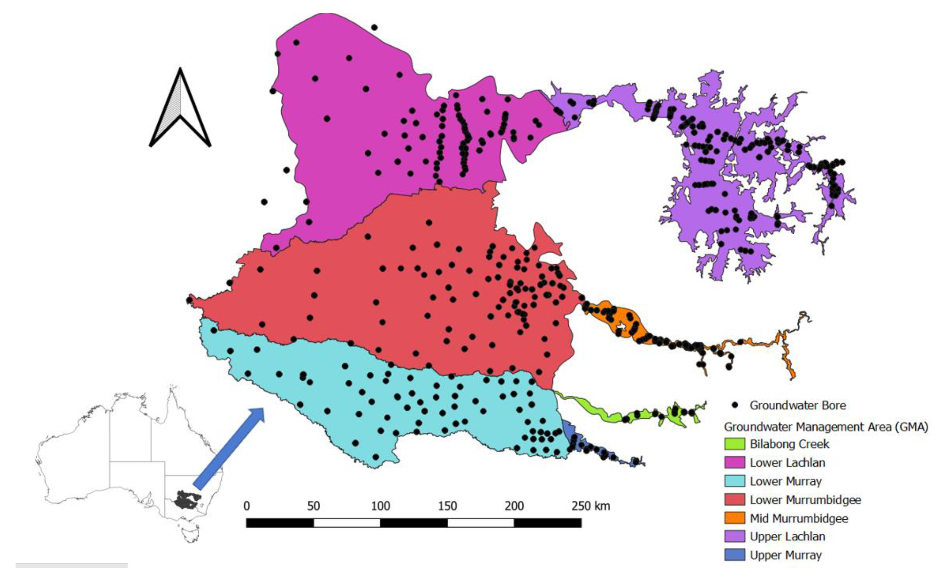
2.1. Study Region

The study area is located in southeast Australia in the state of New South Wales (NSW, Figure 1), where a severe and prolonged dry period occurred in 1997–2009, which is generally referred to as the Millennium Drought [19]. This drought event, together with increasing groundwater extraction, has contributed to and added to the significant groundwater depletion observed in the last 50 years [20]. Ground deformation that occurs as a result of irreversible, inelastic compaction that follows dewatering is of concern for the NSW state government. Protecting the structural integrity of aquifers and aquitards and potentially restricting extraction upon the evidence of irreversible, inelastic compaction are explicit regulatory objectives [21,22]. As many areas in this region are indeed characterized by long-term groundwater abstraction leading to widespread dewatering, the regulator has a need for evidence of any subsequent compaction. However, as groundwater extraction is only one of many factors that may influence deformation, this study did not only explore the temporal correlations between InSAR displacements and groundwater dynamics but also its spatial variations as well as its various influential factors. Contextual information about the study region and the background of this research can be found in the project report [23].
The study region encompassed three major Groundwater Management Areas (GMAs) of the NSW Riverina and several smaller upstream GMAs: Lower and Upper Lachlan (LL, UL), Lower and Mid Murrumbidgee (LMB, MMB), and Lower and Upper Murray, as well as Billabong Creek (LM, UM, BC, Figure 1).

2.2. Groundwater Dynamics

Groundwater depletion is one of the most common factors leading to ground displacements. For example, Zhang et al. [4] have shown that the main cause of land subsidence in Beijing, the capital city of China, is intensive groundwater extraction. Chaussard et al. [24] have demonstrated that groundwater extraction for agricultural and urban activities is the main cause of land subsidence in Mexico.
Two indicators of groundwater dynamics in 975 bores were used in this study: groundwater levels and critical heads (Figure 1). Critical heads (CH) are the historical minima of head levels in an aquifer and a proxy for pre-consolidation heads, which leads to deformation and controls the state of consolidation in fine-grained sediment interbeds and aquitards. Critical head analysis was performed in 416 bores (a subset of the 975 bores with sufficient historical records). Groundwater levels, which represent the aggregation of different hydrogeological processes, including hydroclimate conditions and groundwater extraction [20], were correlated in this study with deformation in order to determine where in space and at which aquifer depths groundwater oscillations could lead to elastic compaction and expansion observed at the ground surface by InSAR.
Critical heads were used in this study based on the assumption that any water level fluctuation above this critical head was assumed to solely influence elastic compaction and expansion. In turn, any new drop in the water levels below previous critical heads established new critical heads and may have created both elastic deformation and inelastic subsidence.
The primary expectation and hypothesis are that critical head drops in aquifers indicate pressure losses in aquitards, which drive inelastic subsidence. However, whether the presence of inelastic subsidence actually translates into InSAR deformation depends on whether the InSAR signal is clouded by other factors, such as elastic expansion/compaction caused by groundwater head oscillations above critical heads, clay swelling/shrinking, other surface factors, and InSAR measurement noise.

2.3. Ground Displacements from InSAR

Radar interferometry, or InSAR, uses the phase observations of a Synthetic Aperture Radar (SAR) sensor to retrieve information about the change in distance between the sensor’s antenna and the ground. By using radar image time series acquired from the same orbital position, the distance change can be interpreted as a modification of the ground level. Information on how the radar images are processed and post-processed to produce deformation maps can be found in [23,25]. Three Sentinel-1 swaths with a total number of 396 acquisitions (132 acquisition dates for each swath) were used and merged and the Intermittent Small Baseline Subset-InSAR. The ISBAS phase-to-deformation inversion strategy was adopted [23,25].

2.4. Correlation between Ground Displacment and Ground Water Level/Critical Head

A correlation analysis was used to explore the relationship between InSAR-derived deformation and groundwater. It is a statistical technique to understand the association between one independent variable (such as groundwater level or critical head) and one continuous dependent variable (such as InSAR-Derived deformation) [26]. In this study, Pearson’s correlation coefficient (r) (Figure 2) was used to explore possible temporal relationships between ground displacement derived from InSAR and groundwater dynamic indicators, i.e., groundwater level and critical head drop time series.
The aim of this analysis was to determine whether InSAR deformation might be influenced by inelastic compaction or elastic deformation because of a critical head drop above the pre-consolidation head or head fluctuations, respectively. As stated above, this analysis was based on a single variable, and as such, it did not directly account for non-groundwater parameters. However, the influence of non-groundwater parameters was inherently integrated into the analysis in the sense that will influence the groundwater/deformation correlation coefficients.

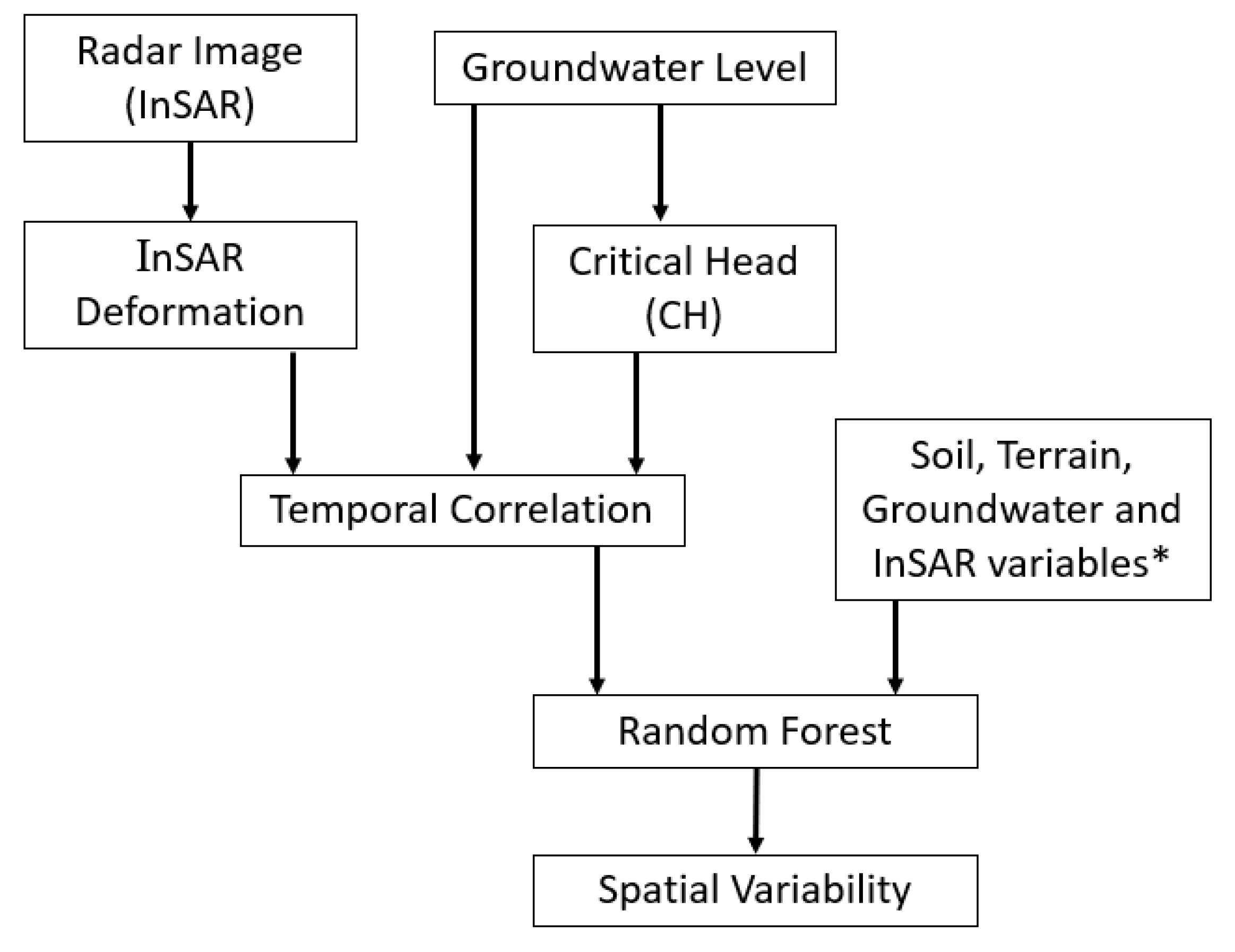
2.5. Random Forest Model of Spatial Variations of Temporal Correlation Coefficients

Random Forest (RF) is a machine-learning algorithm that was originally proposed by Ho [27] and then further developed by Breiman [28,29]. It is a novel ensemble of classification and/or regression trees underpinned by the bootstrapping subset selection technique, in which a model (or a tree) uses a random subset of the observations and controlling predictors to learn the pattern of the given data and attain the best prediction. In other words, many trees (models) are constructed in a certain “random” way to form a Random Forest. The advantage of the RF method is that it can reduce the correlation between decision trees by randomly selecting samples and features to overcome the overfitting issue of decision trees, thereby significantly improving the performance of the final model [2]. Given its advantages, RF has been widely used in practice from financial (such as the bank industry, stock market) to healthcare and medicine sectors (such as breast cancer prediction) and from e-commerce (such as price optimization) to professional sports (such as sports-related injury identification).
In this study, a multi-factorial RF analysis was used to explain the spatial variability of the temporal correlations between ground deformation and the groundwater/critical head (Figure 2). Note that the RF analysis here did not aim at predicting the spatial variability of InSAR deformation itself but the variability in the temporal relationship between InSAR deformation and critical head/groundwater level (Figure 2). The analysis used a set of explanatory variables sorted into four categories: surficial soils, terrain, groundwater, and InSAR-deformation measurement noise as a proxy for land use and land cover (Table 1 and Figure 2). This analysis may provide some answers as to which predictors/variables have an impact on spatially distributed temporal correlations between InSAR deformation and critical heads/groundwater levels over the observation period.
Table 1. Variables of random forest (RF) model.
Type of
Covariates
AcronymDefinitionSource
Surficial soilsClay05Fractional clay content for the soil layer 0–5 cmSoil and Landscape Grid Australia [30]
Clay200Fractional clay content for the soil layer 5–200 cmSoil and Landscape Grid Australia [30]
SoilMoist.TrendTrend in moisture content in 1st meter of soilAustralian Landscape Water Balance model (AWRA-L v6; [31])
SoiMoist.MeanMean moisture content in 1st meter of soilAustralian Landscape Water Balance model (AWRA-L v6; [31])
SoilMoist.DiffDifference between mean moisture content in 1st meter of soil and the corresponding 2005–2015 mean valueAustralian Landscape Water Balance model (AWRA-L v6; [31])
SoilMoist.AmpMaximum amplitude of the moisture variations in 1st meter of soilAustralian Landscape Water Balance model (AWRA-L v6; [31])
SoilClassification of soil typesAustralian Soil Classification (ASC) soil type map of NSW
TerrainSlopeTerrain slopeCalculated from ALOS-3D Digital Elevation Model [32]
ErodibilityMean annual hillslope erosion (tons/ha/year) with C-factorNSW-DPIE, Modelled Hillslope Erosion over New South Wales
Dist.StreamEuclidian distance to streamCalculated from a map of perennial and major streams
ElevationElevation in meters aslALOS-3D Digital Elevation Model [32]
GroundwaterScreen.DepthDepth of the screen for each wellNSW-DPIE
GWExrtactionLayer1Groundwater extraction in the upper aquiferNSW-DPIE
GWExrtactionLayer2Groundwater extraction in the intermediary
aquifer
NSW-DPIE
GWExrtactionLayer3Groundwater extraction in the deep aquifersNSW-DPIE
InSARInter.PercPercentage of quality interferogramsCSIRO—InSAR processing
Spatial.CCMean spatial InSAR coherence, based on 150
randomly selected interferogram for each InSAR stacks
CSIRO—InSAR processing
Temp.CCTemporal InSAR coherence, or ‘stack’ coherenceCSIRO—InSAR processing
The predictors used in the RF analysis examined the overall value of each factor to predict the temporal correlation between InSAR deformation and critical head/groundwater level for the entire InSAR period and over the entire study area. That is, the RF analysis uses static and time-integrated variables (totals, means, or trends for time-variable variables). As the analysis explained the correlations between ground deformation and well information (groundwater levels and critical heads), this is dependent on such data and could not lead to extrapolation beyond locations where the groundwater data was available.

3. Results

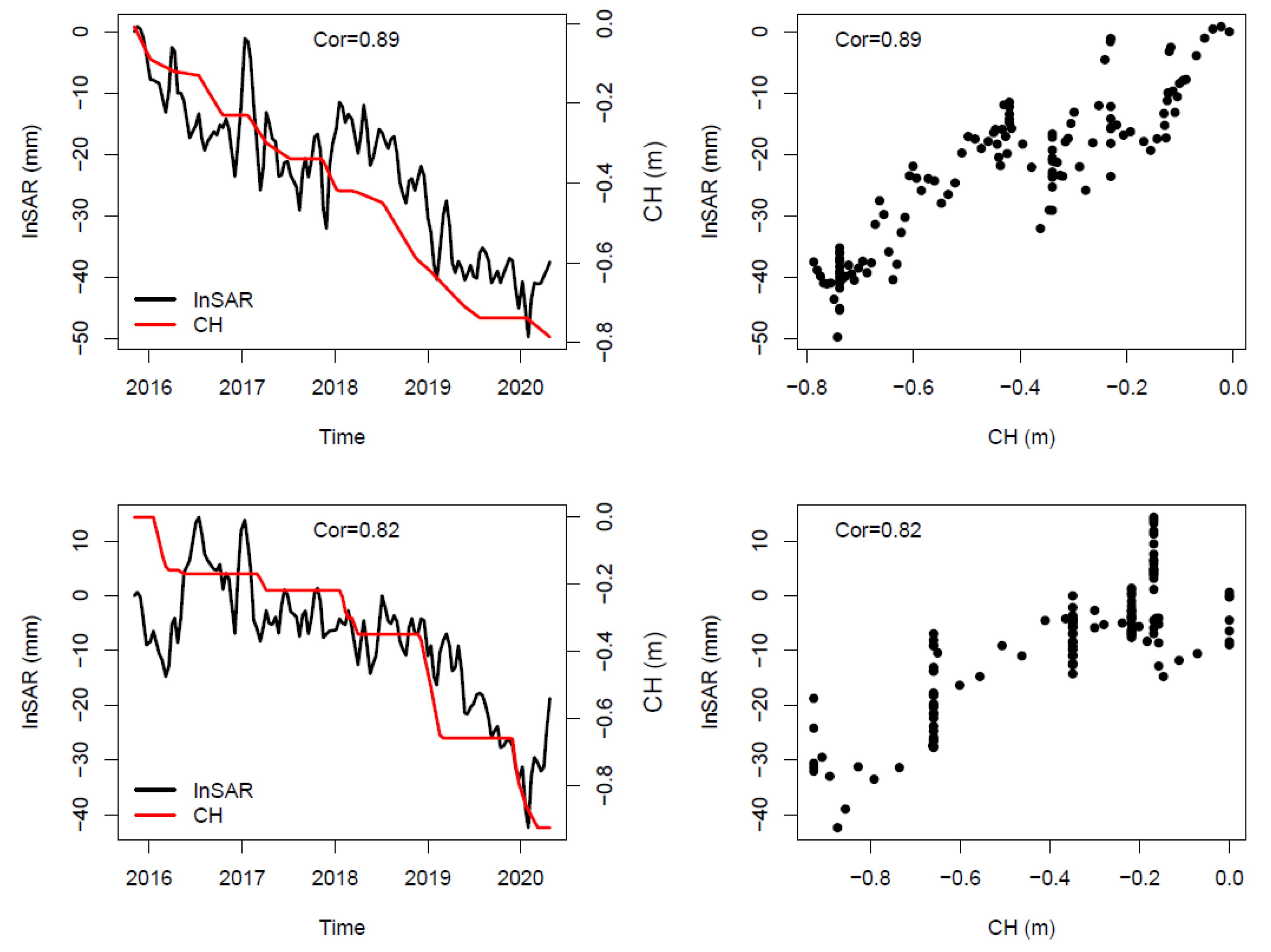
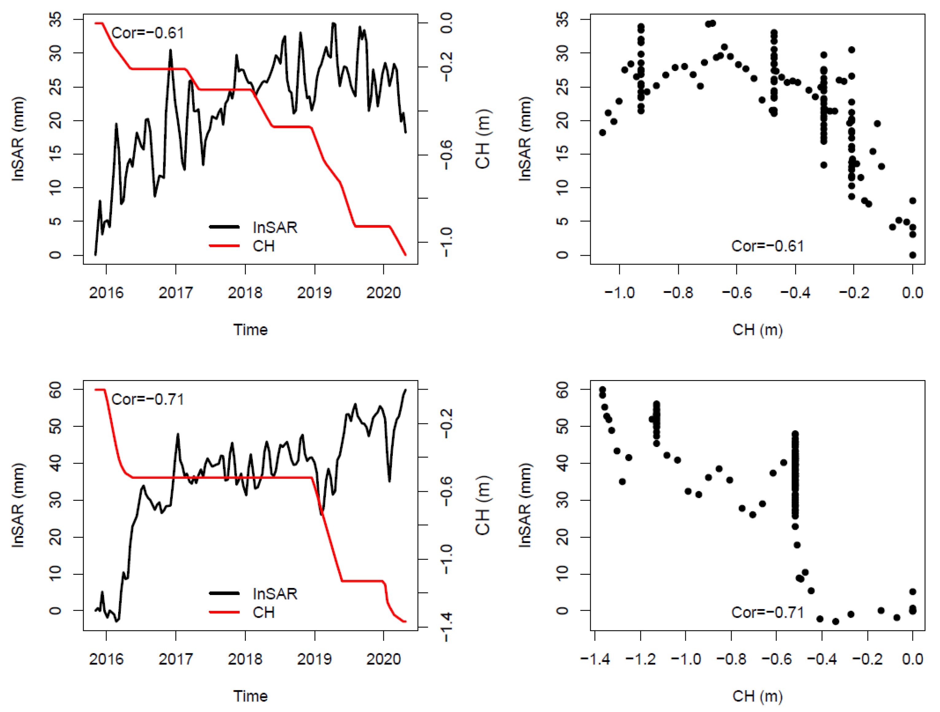
3.1. Temporal Correlations between InSAR Displacements and Groundwater Critical Head Drop

Table 2 shows the summary of correlation coefficients between InSAR and the critical head drop time series from 416 piezometers with sufficient historical records. Overall, it was skewed towards a positive relationship (75.5%) between InSAR and critical head drop, implying that critical head was an important factor for InSAR displacement. While a positive correlation was expected where groundwater extraction induced the compaction of the fine-grained sediments present in the aquifer system, a negative correlation was theoretically possible if depletion of the surficial aquifer induced geostatic unloading and the expansion of the underlying confined aquifer. In that case, groundwater depletion in the surficial aquifer led to the uplift of the ground surface.
Figure 3 shows two examples of the strong and positive correlation between InSAR and the critical head time series (Cor = 0.89 and 0.82), which supports the hypothesis that, for some piezometers, the critical head is an important contributor to InSAR displacement. In contrast, Figure 4 demonstrates two cases of a negative correlation between InSAR and the critical head, i.e., a decline in the critical head with a positive InSAR displacement. A negative correlation could also have hydrogeological implications. Depleting a surficial aquifer can cause the expansion of the confined aquifer below, and accordingly, a negative correlation could be observed between the surficial aquifer level time series and the InSAR deformation time series (Figure 4). However, a negative correlation could also imply that surface factors rather than groundwater dynamics could result in InSAR displacement (Figure 3). These two figures are just examples of strong positive and negative correlations and, in fact, the majority of the bores show a correlation coefficient in the intermediary value range, as shown in Table 2. A very weak correlation most likely indicated that surface factors rather than groundwater dynamics led to InSAR displacement or that groundwater pressure did not lead to ground deformation at that location.

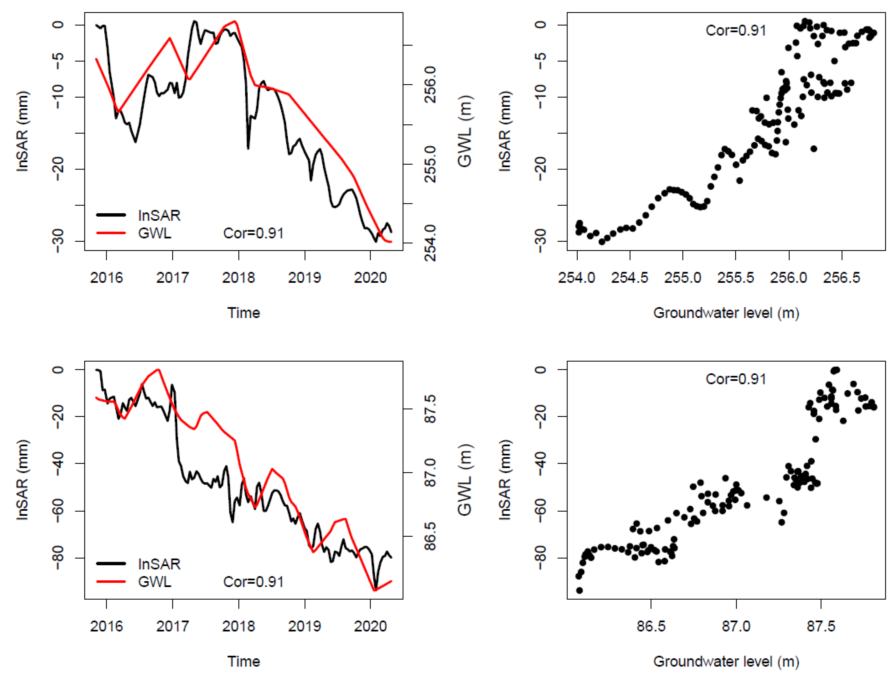
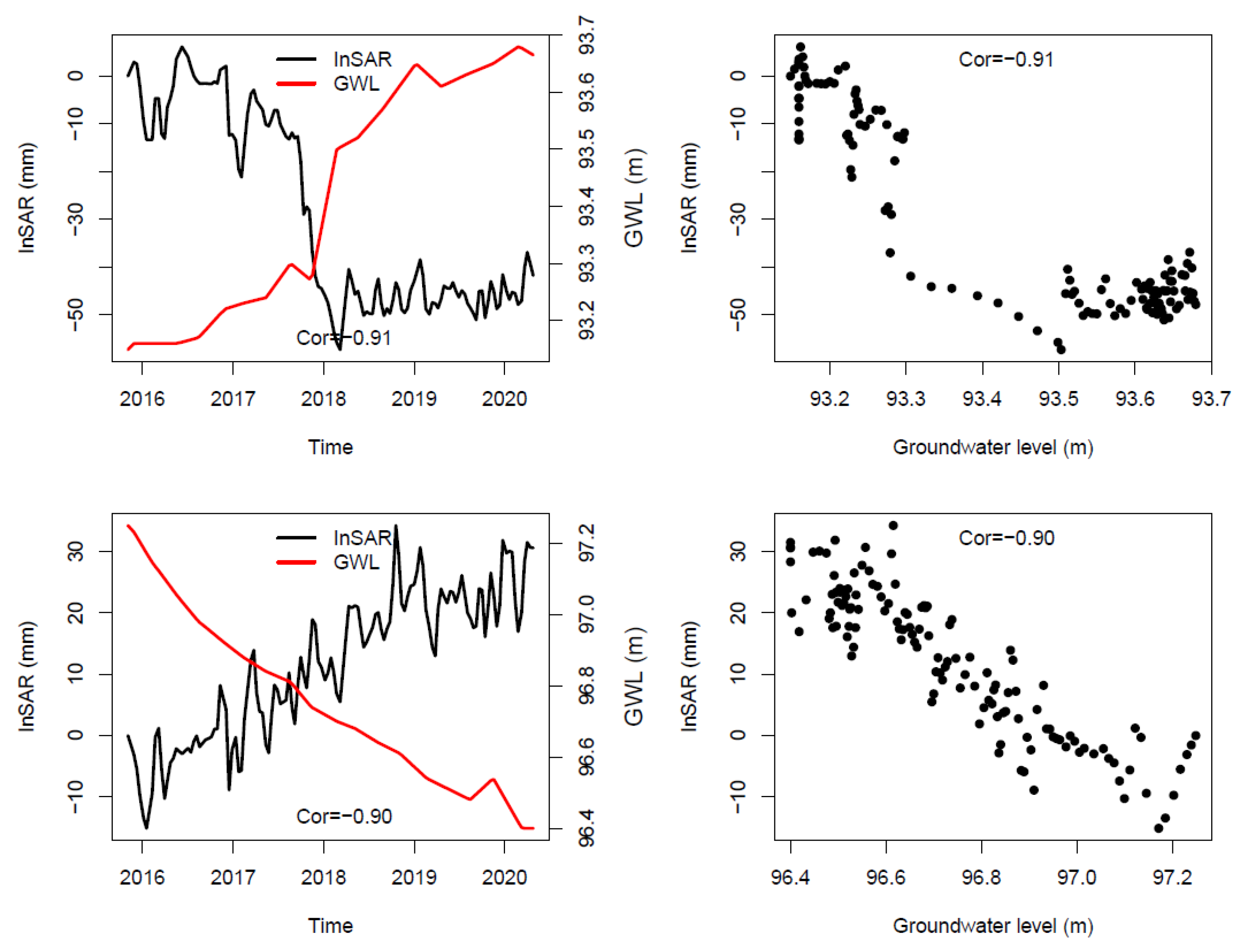
3.2. Temporal Correlations between InSAR Displacements and Groundwater Level

Table 3 shows a summary of correlation coefficients between the InSAR displacement time series and groundwater head time series (referred to as groundwater level, GWL) in 975 bores. The number of groundwater bores with groundwater level observations was much larger (975 vs. 416) than that with a critical head drop, given that no historical data before the InSAR temporal window was required for this analysis. Overall, this was also skewed towards a positive relationship between the InSAR and GWL time series in the last 5 years, highlighting the groundwater level contribution to InSAR displacements. However, 237 piezometers still showed a negative correlation between InSAR and groundwater level.
Figure 5 shows two examples of strong, positive correlations between InSAR displacement and GWL (Cor = 0.91 and 0.91). Both InSAR displacement and GWL showed decreasing trends over the last 5 years, implying that the InSAR deformation was driven by elastic aquifer compaction and expansion. In contrast, Figure 6 shows two piezometers with a negative correlation between both positive and negative InSAR displacements and declining/increasing GWL trends. While a negative correlation could also have implications between InSAR and groundwater level due to the expansion of the confined aquifer, it could also indicate that surface factors, such as rainfall, evapotranspiration, land use/land cover change and groundwater recharge, rather than groundwater dynamics could affect InSAR displacement (Figure 6).

3.3. Spatial Variability of Temporal Correlations between InSAR Displacements and Groundwater Critcal Head Drop and Its Predictors with RF

The RF model could explain 71.7% of the spatial variance of temporal correlation between InSAR displacement and groundwater head drop with 18 predictors, as shown in Table 1, which was superior compared to a simple linear regression model with the same 18 variables that could only explain 28.6% of the variance (R2 = 0.286). However, it should be noted that the 18 land cover classes, soil, and terrain covariates explained the variance in the spatial distribution of all correlations between the groundwater and deformation, ranging from positive to negative. Hence, naturally, surface factors that lead to an upward displacement while, at the same time, a drop in groundwater was recorded also play a role in this result. The relative importance of RF (Figure 7) indicated that spatial InSAR coherence (Spatial.CC; a proxy for noise in InSAR data, its spatial patterns are mainly controlled by the land cover) and soil moisture (difference, trend, and amplitude) were the four most important factors resulting in a spatial pattern of correlation between InSAR displacement and critical head changes.
The left panel of Figure 7 shows a mean decrease in accuracy (%IncMSE) if we leave out a particular variable, and the right panel shows a mean decrease in the Mean Squared Error (MSE) (IncNodePurity), which is a measurement of variable importance based on the Gini impurity index, which was used for the calculation of the splits in RF trees. The higher the value of the mean decreased accuracy or mean decreased Gini score, the higher the importance of the variable was in the model. The top five variables were the same based on these two criteria, although in slightly different orders.
An RF model with these four important factors was then built, and it could explain a 67.5% variance in the spatial distribution of the temporal correlation, which was close to the 71.7% variance of the full model with 18 predictors. Another RF model with only three soil moisture variables was also built, and it could explain 65.2% pf the spatial variance of temporal correlation between InSAR displacement and critical head. This is only slightly worse than the four-predictor model (−2.3%). This comparison was valid with the same random seed, given the “random” characteristics of the RF method. This indicates that the characteristics of soil moisture are critically important to explain the temporal correlations between InSAR displacement and critical head. However, the RF model slightly underpredicted the positive correlation values between InSAR displacement and critical heads and overpredicted the negative correlation values (Figure 8).

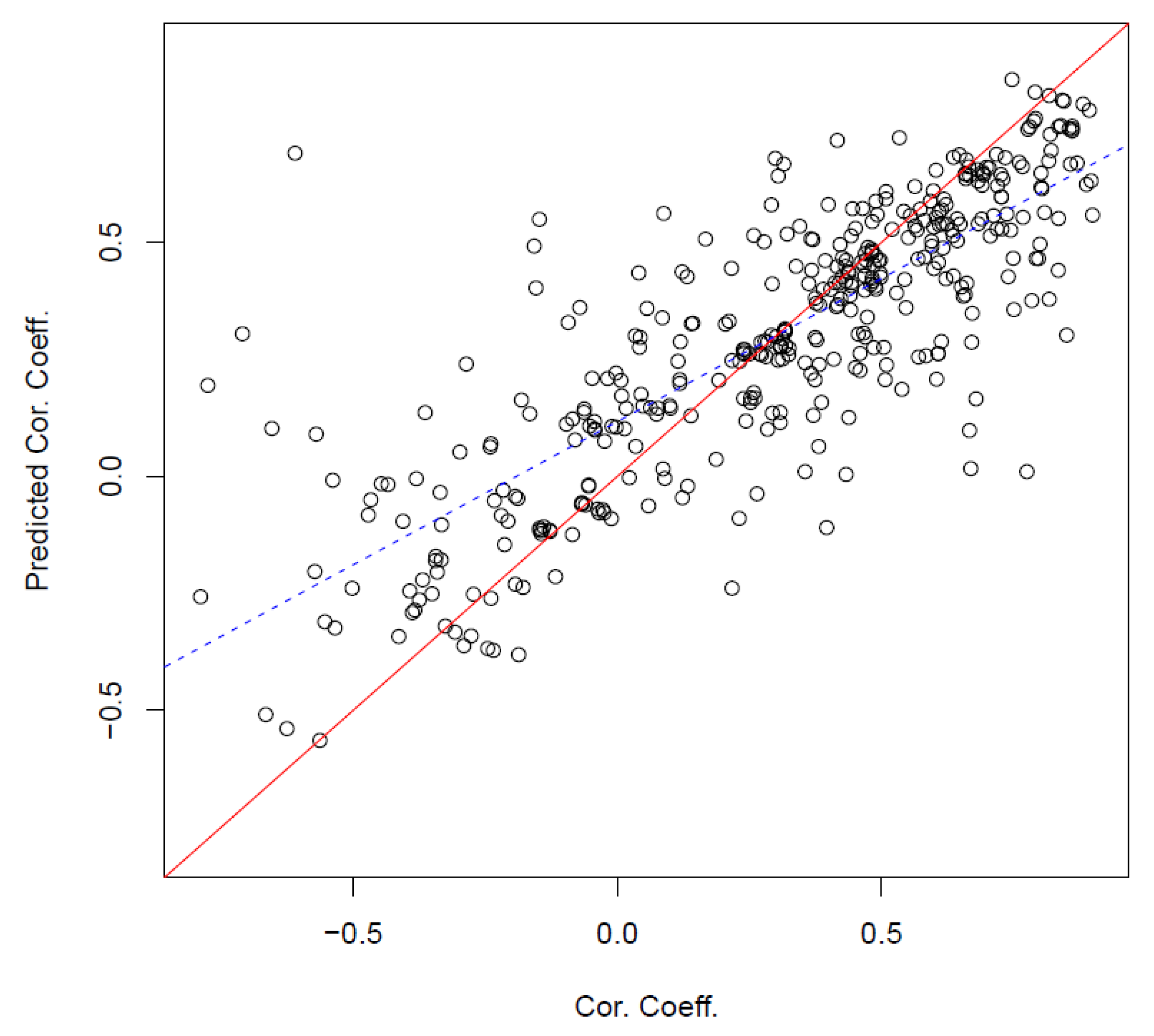
3.4. Spatial Variability of Temporal Correlations between InSAR Displacements and Groundwater Level and Its Predictors with RF

The RF spatial model of the temporal correlation between InSAR displacement and groundwater level with 18 predictors could explain 60.0% of the spatial variance, which is also much better than a linear regression model with the same 18 variables that could only explain 9.7% of the variance (R2 = 0.097). These two values were lower than their corresponding values between InSAR displacements and critical heads, i.e., 71.7% vs. 60.0% and 28.6% vs. 9.7%. However, a lower value does not necessarily indicate a poorer RF model given the different sample sizes, i.e., 416 vs. 975.
The relative importance of RF (Figure 9) indicates temporal and spatial InSAR coherence (Temp.CC and Spatial.CC; both are proxies for the decorrelation of the radar signal and noise in InSAR data) and soil moisture (difference, trend and amplitude) and are the most important factors resulting in a spatial pattern of temporal correlation. However, it should be noted that different rankings for variable importance could be obtained based on two different criteria. For example, the screen depth of a bore (Screen.Depth) is the second most important variable to explain the spatial variance of correlation between InSAR displacements and groundwater levels based on IncNodePurity but was only ranked 10th out of 18 variables based on %IncMSE (Figure 9). In theory, there was not a fixed criterion that could be considered as the “best” measure of variable importance.

4. Discussion

4.1. Advantages of RF Model

The RF machine learning technique was useful to investigate the spatial distribution of temporal correlation between InSAR and critical head/groundwater level and their contributing factors. It produced a much higher correlation coefficient compared to traditional linear regression because it could capture the complex and non-linear relationship between predict and (temporal correlation coefficient between InSAR and critical head/groundwater level) and the predictors (Table 1). This is consistent with conclusions found in the literature [2,9,10,11,12,13,14,15,16,17,18].
The model was robust. For example, the 3-predictor RF model was run 1000 times to quantify the random characteristics of the RF method, and it showed that it was a robust model with a variance explained below 65.0–67.9% (Figure 10).

4.2. Limitations and Uncertainty of RF Model

One major caveat of the RF model is that it is a machine-learning algorithm, not a physical process-based model. It is possible that different combinations of predictors could result in similar models, i.e., non-uniqueness, and that some of the results are difficult to explain from a physical process point of view. It could also be part of the reason why different studies have identified different important variables, leading to ground deformation (Table 4).
The controlling factors of InSAR-derived ground deformation are complex and vary from region to region depending on many factors, such as local hydrogeological settings, hydroclimate conditions, lithology, land use and land cover, elevation modeling errors, soil moisture and texture changes. It is potentially part of the reason why many bores have a weak correlation between InSAR displacement and groundwater level/critical head drop.
The RF model was run based on deformation and head observations at monitoring bore locations only because we targeted the temporal correlation between InSAR displacement and the critical head/groundwater level. The results indicated that soil moisture variables (3 statistics) were among the most important contributor to explaining the spatial variability of temporal correlations between InSAR displacement and the critical head. If the relationships between the soil moisture and temporal correlation could be explained as a physically-based process, then the spatial distribution of temporal correlation could be predicted with the soil moisture and the RF model. Given the potentially serious damage to farms and urban infrastructure and other environmental issues that land subsidence could cause, a prediction model was useful for practical applications or as a decision-support basis.
The RF model could also be run for each individual year (5-year data implies five different RF models) because the hydroclimate conditions varied from year to year or each groundwater management area, which could tell us whether the most important contributing factors were different within wet/dry climate conditions and different groundwater management areas.
More importantly, the RF model could be run for individual GMAs, which would help the model account for the variability of lithological parameters that are under-represented in the analysis presented in this paper, e.g., compressibility, thickness of aquitards and fine-grained interbeds. Such an analysis could assume that lithology was less heterogenous at the GMA scale rather than at the scale of the entire study area. In addition, the temporal correlation between InSAR displacements and groundwater level/critical head showed a spatial pattern. For example, the piezometers in the Upper Lachlan and Lower Murrumbidgee (Figure 1) generally showed a combination of larger negative GWL trends and a larger declining InSAR trend [23].
Only one RF model for the seven groundwater management areas (GMAs) was produced, with lithological heterogeneity largely unaccounted for in the set of covariates (Table 1), which led to an inherent underestimation of the influence of lithological factors in the RF analysis. Individual RF models at scales solely where the correlation between the groundwater level declined, deformation was positive, and where the lithology is homogeneous could potentially provide a more meaningful determination of influential covariates.
Nevertheless, even at a regional scale across all seven GMAs, a competent model with R2 > 0.7 could be built using the proposed set of covariates, which reinforced the idea that both surficial soils and InSAR noise (due to radar phase decorrelation and residuals of deformation model fitting) were important contributing factors to the InSAR results; thus, it influenced the temporal correlation with groundwater level changes. More generally, we noted that the RF machine learning technique was useful for investigating the spatial distribution of correlation between InSAR and critical head/groundwater level and their contributing factors.
Last, but not the least, the entire dataset was used to build the spatial RF model and was not split into calibration and validation subsets. This was because the aim of this analysis was to explore contributing factors controlling the spatial patterns of the Pearson coefficient of correlation between InSAR and groundwater dynamics. That is to say, the objective of this study was not to build a prediction model to map the spatial distribution of ground displacement.

5. Conclusions

Ground displacement or ground deformation and associated horizontal deformation often have significant damaging effects, such as damage to infrastructure and increased exposure to flooding. This has been observed in many countries in the world and has attracted great attention because of its impacts and implications.
Results from the interferometric synthetic aperture radar (InSAR) technique were used in this study to derive the temporal and spatial information of land subsidence in southeast Australia. Temporal correlations between InSAR displacement and groundwater level dynamics were analyzed. Groundwater dynamics can be considered an important factor for InSAR displacement temporal evolution where strong positive correlations are observed. However, a negative correlation between InSAR displacement and groundwater dynamics can also be observed for other bores, potentially due to the expansion of the confined aquifer. It may also indicate that surface factors unrelated to groundwater, such as rainfall, evapotranspiration, land use/land cover change and groundwater recharge, rather than groundwater dynamics, could affect InSAR displacement, especially if their correlation is very weak.
The random forest (RF) machine learning method was used to model the spatial variation in the temporal correlations between InSAR displacement and groundwater dynamics. The results indicate that the RF model was a useful tool with which to investigate the spatial distribution of temporal correlation, and it could explain 71.7% and 60.0% spatial variances between the InSAR and critical head/groundwater level, respectively. The RF models also produced a higher correlation coefficient compared to traditional linear regression because it captured the complicated and non-linear relationship between the predict and (temporal correlations between InSAR displacements and groundwater levels) and predictors (soil, terrain, and groundwater variables).
The 3-predictor RF model was run 1000 times to quantify the random characteristics of the RF method and showed that it was a robust model with variance explained below 65.0–67.9%.
The spatial and temporal InSAR coherence (a proxy for noise in InSAR data that is mainly related to land cover and model fitting performance, respectively) and soil moisture (difference, trend, and amplitude) were the most important factors resulting in the spatial pattern of correlations between InSAR displacements and groundwater dynamics (critical head or groundwater level changes). This result confirmed that the influence from surficial soils (clay content, moisture changes) should be accounted for while interpreting InSAR data.
The limitations and uncertainties include but are not limited to (a) RF is not a physical process-based model and some results are difficult to explain; (b) The model can only be run at monitoring bore locations due to data availability; (c) The mixed wet/dry hydroclimate conditions are merged into a single model; and (d) a combined model is built for different groundwater management areas with various lithological and hydrogeological settings.
The RF machine learning results provide added value to the correlation analysis for suggesting a ranking of spatially distributed influential variables that can explain and model the correlation between deformation and groundwater dynamics. However, given that both positive and negative correlations are included in this study, the predictive value of the analysis has limitations. These could be partially overcome by focusing RF analyses on subsets of the domain at scales where clusters of positive or negative correlation between groundwater level decline and deformation are dominant or for specific GMAs, where the lithology could be considered homogeneous.

Author Contributions

Conceptualization, G.F., W.S. and P.C.; methodology, G.F. and W.S.; software, G.F.; validation, G.F., W.S. and P.C.; formal analysis, G.F.; investigation, G.F., W.S. and P.C.; data curation, W.S. and P.C.; writing—original draft preparation, G.F., W.S. and P.C.; writing—review and editing, G.F., W.S. and P.C.; funding acquisition, W.S. All authors have read and agreed to the published version of the manuscript.

Funding

This research was funded by the New South Wales Department of Planning, Industry & Environment (NSW DPIE) Water Group.

Data Availability Statement

The original radar data can be downloaded from the Alaska Satellite Facility (https://search.asf.alaska.edu/). The processed InSAR results are available from authors upon request. The groundwater level data was provided by New South Wales Department of Planning, Industry & Environment (NSW DPIE) Water Group.

Acknowledgments

We would like to thank the NSW DPIE Water Group (in particular Prem Kumar) for sharing data and technical assistance.

Conflicts of Interest

The authors declare no conflict of interest.

References

  1. Galloway, D.L.; Burbey, T.J. Review: Regional land subsidence accompanying groundwater extraction. Hydrogeol. J. 2011, 19, 1459–1486. [Google Scholar] [CrossRef]
  2. Chen, B.B.; Gong, H.L.; Chen, Y.; Li, X.J.; Zhou, C.F.; Lei, K.C.; Zhu, L.; Duan, L.; Zhao, X.X. Land subsidence and its relation with groundwater aquifers in Beijing Plain of China. Sci. Total Environ. 2020, 735, 139111. [Google Scholar] [CrossRef] [PubMed]
  3. Parker, A.L.; Filmer, M.S.; Featherstone, W.E. First Results from Sentinel-1A InSAR over Australia: Application to the Perth Basin. Remote Sens. 2017, 9, 299. [Google Scholar] [CrossRef]
  4. Zhang, Y.Q.; Gong, H.L.; Gu, Z.Q.; Wang, R.; Li, X.J.; Zhao, W.J. Characterization of land subsidence induced by groundwater withdrawals in the plain of Beijing city, China. Hydrogeol. J. 2014, 22, 397–409. [Google Scholar] [CrossRef]
  5. Raucoules, D.; Cartannaz, C.; Mathieu, F.; Midot, D. Combined use of space-borne SAR interferometric techniques and ground-based measurements on a 0.3 km(2) subsidence phenomenon. Remote Sens Env. 2013, 139, 331–339. [Google Scholar] [CrossRef]
  6. Solari, L.; Ciampalini, A.; Raspini, F.; Bianchini, S.; Zinno, I.; Bonano, M.; Manunta, M.; Moretti, S.; Casagli, N. Combined Use of C- and X-Band SAR Data for Subsidence Monitoring in an Urban Area. Geosciences 2017, 7, 21. [Google Scholar] [CrossRef]
  7. Castellazzi, P.; Arroyo-Dominguez, N.; Martel, R.; Calderhead, A.I.; Normand, J.C.L.; Garfias, J.; Rivera, A. Land subsidence in major cities of Central Mexico: Interpreting InSAR-derived land subsidence mapping with hydrogeological data. Int. J. Appl. Earth Obs. Geoinf. 2016, 47, 102–111. [Google Scholar] [CrossRef]
  8. Lu, Z.; Dzurisin, D.; Biggs, J.; Wicks, C.; McNutt, S. Ground surface deformation patterns, magma supply, and magma storage at Okmok volcano, Alaska, from InSAR analysis: 1. Intereruption deformation, 1997–2008. J. Geophys. Res. Solid Earth 2010, 115, B00B02. [Google Scholar] [CrossRef]
  9. Ilia, I.; Loupasakis, C.; Tsangaratos, P. Land subsidence phenomena investigated by spatiotemporal analysis of groundwater resources, remote sensing techniques, and random forest method: The case of Western Thessaly, Greece. Environ. Monit. Assess. 2018, 190, 623. [Google Scholar] [CrossRef]
  10. Choubin, B.; Mosavi, A.; Alamdarloo, E.H.; Hosseini, F.S.; Shamshirband, S.; Dashtekian, K.; Ghamisi, P. Earth fissure hazard prediction using machine learning models. Environ. Res. 2019, 179, 108770. [Google Scholar] [CrossRef]
  11. Mohammady, M.; Pourghasemi, H.R.; Amiri, M. Land subsidence susceptibility assessment using random forest machine learning algorithm. Environ. Earth Sci. 2019, 78, 503. [Google Scholar] [CrossRef]
  12. Rahmati, O.; Falah, F.; Naghibi, S.A.; Biggs, T.; Soltani, M.; Deo, R.C.; Cerda, A.; Mohammadi, F.; Bui, D.T. Land subsidence modelling using tree-based machine learning algorithms. Sci. Total Environ. 2019, 672, 239–252. [Google Scholar] [CrossRef] [PubMed]
  13. Zamanirad, M.; Sarraf, A.; Sedghi, H.; Saremi, A.; Rezaee, P. Modeling the Influence of Groundwater Exploitation on Land Subsidence Susceptibility Using Machine Learning Algorithms. Nat. Resour. Res. 2020, 29, 1127–1141. [Google Scholar] [CrossRef]
  14. Arabameri, A.; Saha, S.; Roy, J.; Tiefenbacher, J.P.; Cerda, A.; Biggs, T.; Pradhan, B.; Ngo, P.T.T.; Collins, A.L. A novel ensemble computational intelligence approach for the spatial prediction of land subsidence susceptibility. Sci. Total Environ. 2020, 726, 138595. [Google Scholar] [CrossRef]
  15. Chatrsimab, Z.; Alesheikh, A.A.; Voosoghi, B.; Behzadi, S.; Modiri, M. Development of a Land Subsidence Forecasting Model Using Small Baseline Subset-Differential Synthetic Aperture Radar Interferometry and Particle Swarm Optimization-Random Forest (Case Study: Tehran-Karaj-Shahriyar Aquifer, Iran). Dokl. Earth Sci. 2020, 494, 718–725. [Google Scholar] [CrossRef]
  16. Ebrahimy, H.; Feizizadeh, B.; Salmani, S.; Azadi, H. A comparative study of land subsidence susceptibility mapping of Tasuj plane, Iran, using boosted regression tree, random forest and classification and regression tree methods. Environ. Earth Sci. 2020, 79, 223. [Google Scholar] [CrossRef]
  17. Elmahdy, S.I.; Mohamed, M.M.; Ali, T.A.; Abdalla, J.E.; Abouleish, M. Land subsidence and sinkholes susceptibility mapping and analysis using random forest and frequency ratio models in Al Ain, UAE. Geocarto Int. 2022, 37, 315–331. [Google Scholar] [CrossRef]
  18. Arabameri, A.; Pal, S.C.; Rezaie, F.; Chakrabortty, R.; Chowdhuri, I.; Blaschke, T.; Ngo, P.T.T. Comparison of multi-criteria and artificial intelligence models for land-subsidence susceptibility zonation. J. Env. Manag. 2021, 284, 112067. [Google Scholar] [CrossRef]
  19. Fu, G.; Chiew, F.H.S.; Post, D.A. Trends and variability of rainfall characteristics influencing annual streamflow: A case study of southeast Australia. Int. J. Climatol. 2023, 43, 1407–1430. [Google Scholar] [CrossRef]
  20. Fu, G.B.; Rojas, R.; Gonzalez, D. Trends in Groundwater Levels in Alluvial Aquifers of the Murray-Darling Basin and Their Attributions. Water 2022, 14, 1808. [Google Scholar] [CrossRef]
  21. NSW. Water Resource Plans. Available online: https://www.industry.nsw.gov.au/water/plans-programs/water-resource-plans (accessed on 5 April 2023).
  22. NSW. Water Sharing Plans. Available online: https://www.industry.nsw.gov.au/water/plans-programs/water-sharing-plans (accessed on 5 April 2023).
  23. Castellazzi, P.; Schmid, W.; Fu, G. Ground Displacements Over Alluvial Aquifers in Southern Inland New South Wales; CSIRO: Canberra, Australia, 2021; p. 67. [Google Scholar] [CrossRef]
  24. Chaussard, E.; Wdowinski, S.; Cabral-Cano, E.; Amelung, F. Land subsidence in central Mexico detected by ALOS InSAR time-series. Remote Sens. Environ. 2014, 140, 94–106. [Google Scholar] [CrossRef]
  25. Castellazzi, P.; Schmid, W.; Fu, G. Exploring the potential for groundwater-related ground deformation in Southern New South Wales, Australia. Sci. Total Environ. 2023; under review. [Google Scholar]
  26. Fu, G.B.; Crosbie, R.S.; Barron, O.; Charles, S.P.; Dawes, W.; Shi, X.G.; Niel, T.V.; Li, C. Attributing variations of temporal and spatial groundwater recharge: A statistical analysis of climatic and non-climatic factors. J. Hydrol. 2019, 568, 816–834. [Google Scholar] [CrossRef]
  27. Ho, T.K. Random decision forests. In Proceedings of the 3rd International Conference on Document Analysis and Recognition, Montreal, QC, USA, 14–15 August 1995; pp. 278–282. [Google Scholar]
  28. Breiman, L. Bagging predictors. Mach. Learn. 1996, 24, 123–140. [Google Scholar] [CrossRef]
  29. Breiman, L. Random forests. Mach. Learn. 2001, 45, 5–32. [Google Scholar] [CrossRef]
  30. Rossel, R.A.V.; Webster, R.; Bui, E.N.; Baldock, J.A. Baseline map of organic carbon in Australian soil to support national carbon accounting and monitoring under climate change. Glob. Chang. Biol 2014, 20, 2953–2970. [Google Scholar] [CrossRef]
  31. Frost, A.J.; Ramchurn, A.; Smith, A. The Australian Landscape Water Balance Model (AWRA-L v6). Technical Description of the Australian Water Resources Assessment Landscape Model; Australian Government Bureau of Meteorology: Melbourne, Australia, 2018.
  32. Tadono, T.; Nagai, H.; Ishida, H.; Oda, F.; Naito, S.; Minakawa, K.; Iwamoto, H. Generation of the 30 M-Mesh Global Digital Surface Model by Alos Prism. Int. Arch. Photogramm. 2016, 41, 157–162. [Google Scholar] [CrossRef]
Figure 1. Location of the study region, groundwater management areas, and groundwater bores.
Geosciences 13 00133 g001
Figure 2. Methodology diagram of this research (* Table 1).
Geosciences 13 00133 g002
Figure 3. Two examples of strong and positive correlations between InSAR deformation and critical head (CH) ((left): time series comparison; (right): correlation scatter plots).
Geosciences 13 00133 g003
Figure 4. Examples of negative correlation between InSAR deformation and critical head (CH) ((left): time series comparison; (right): correlation scatter plots).
Geosciences 13 00133 g004
Figure 5. Examples of strong and positive correlation between InSAR deformation and groundwater level (GWL) ((left): time series comparison; (right): correlation scatter plots).
Geosciences 13 00133 g005
Figure 6. Examples of negative correlation between InSAR deformation and groundwater level ((left): time series comparison; (right): correlation scatter plots).
Geosciences 13 00133 g006
Figure 7. Relative importance of 18 predictors for the spatial variability of temporal correlation between InSAR deformation and groundwater head drop time-series.
Geosciences 13 00133 g007
Figure 8. Temporal correlations between InSAR deformation and critical head vs. RF simulated results (red line is the 1:1 line and blue dash line is the linear fitted line). Each circle represents one groundwater bore.
Geosciences 13 00133 g008
Figure 9. Relative importance of 18 predictors for the spatial variability of the temporal correlation between InSAR deformation and groundwater level time-series.
Geosciences 13 00133 g009
Figure 10. Variance explained with 3-predictor RF model of temporal correlation between InSAR deformation and critical head (1000 runs).
Geosciences 13 00133 g010
Table 2. Correlation coefficients between InSAR and critical head drop time-series observed at 416 bores.
Cor. Coeff.No. of Bores%No. of Bores%
<−0.800.010224.5
−0.8 to −0.5163.8
−0.5 to −0.2389.1
−0.2 to 04811.5
0 to 0.2399.431475.5
0.2 to 0.513732.9
0.5 to 0.811126.7
>0.8276.5
Table 3. Correlation coefficients between InSAR and groundwater level time series.
Cor. Coeff.No. of Bores%No. of Bores%
<−0.850.523724.3
−0.8 to −0.5414.2
−0.5 to −0.2979.9
−0.2 to 0949.6
0 to 0.211712.073875.7
0.2 to 0.525125.7
0.5 to 0.832633.4
>0.8444.5
Table 4. Examples of RF land substance applications and important variables.
StudyModelImprtant Variables
Arabameri et al. (2020) [14]ANN-bagging and RFGroundwater drawdown, land use and land cover, elevation, and lithology
Arabameri et al. (2021) [18]5 AI and conditional RF is the bestLand use/land cover (LULC) (most important factor), Groundwater depth (2nd most important), and lithology, TWI, elevation, slope, aspect, distance to road, drainage density, profile curvature, distance to stream and plan curvature
Chatrsimab et al. (2020) [15]PSO-RFMedia aquifer (furthermost effective factor), groundwater drawdown and transmissivity and storage coefficient
Chen et al. (2020) [2]RFVariation in groundwater level in the second confined aquifer
Choubin et al. (2018) [10]5 ML and RF is the bestLow elevations with characteristics of high groundwater withdrawal, drop in groundwater level, high well density, high road density, low precipitation, and Quaternary sediments distribution
Ilia et al. (2018) [9]RFThickness of loose deposits, the Sen’s slope value of groundwater-level trend, and the Compression Index of the formation covering the area of interest
Mohammady et al. (2019) [11]RFDistance from fault, elevation, slope angle, land use, and water table
Rahmati et al. (2019) [12]4 ML and RF is the bestGroundwater drawdown (the most important)
Lithology, and distance from the stream network
Zamanirad et al. (2020) [13]3 ML and RF benchmarkDrawdown of groundwater level (77.5%); lithology (19.2%), distance from streams (2.5%), and altitude (0.8%).
This studyRFInSAR coherence (a proxy for noise in InSAR data that is mainly caused by
variations in land cover) and soil moisture (difference, trend, and amplitude)
Disclaimer/Publisher’s Note: The statements, opinions and data contained in all publications are solely those of the individual author(s) and contributor(s) and not of MDPI and/or the editor(s). MDPI and/or the editor(s) disclaim responsibility for any injury to people or property resulting from any ideas, methods, instructions or products referred to in the content.

