Automating the Process for Estimating Tunneling Induced Ground Stability and Settlement

Abstract

An automatic process for estimating ground stability and settlement of circular tunnels is developed for practitioners in this paper using finite difference method FLAC code. The numerical model aims to simulate the movement and relaxation of the soil around the shield and lining annulus that occurs due to the overcutting and grouting of the tunnel void by a tunnel boring machine. To achieve this, the model uses a pressure relaxation technique that progressively reduces the tunnel support pressure from the initial at rest condition until a point of failure is detected. At this stage, the stability number is calculated, and settlement data are exported for analysis. This is conducted for a range of geometry and soil ratios which cover most practical cases for cohesive soils. These stability numbers are then compared to rigorous upper and lower bound solutions. Using the settlement data, a trough width parameter i_x is also determined for each case using regression of the commonly used Gaussian equation. The results of this study are quite positive, with the stability results from this study remaining within 5% of the upper and lower bound solutions; settlement results also compare well with previous experimental and observational results. The proposed automatic process can be used effectively and efficiently in most practical design projects.

1. Introduction

Increased urbanization has driven much research into better management of transport services and infrastructure. With limited scope for changes above ground, effective use of the underground space is a targeted solution. Tunnels have become a common solution. Since the development of tunnel boring machines (TBMs) over the past few decades, tunnels can now be produced under very difficult ground conditions, such as very soft ground. In such conditions where the soil mechanics are more critical, responsibility increasingly falls to the geotechnical engineer. According to Peck (1969) [1], the three primary design criteria of underground tunnels from a geotechnical perspective are: stability during construction, long- and short-term settlement, and determination of lining structural loading. Indeed, the inevitable delay between when the tunnel is bored and when the lining and the grout is installed, as well as the overcutting due to the cutting head being of slightly larger diameter than the rest of the TBM, are of great concerns to tunnel engineers (see Figure 1).

Evaluating tunneling stability during its construction is essential. This is most often known by using the stability number (N) proposed by Broms and Bennermark (1967) [2], as shown in Equation (1). Their research was a pilot study of the plastic flow of clay soil in vertical openings of retaining walls. It was then extended to the experimental study of a tunnel face supported by an internal air pressure by Mair (1979) [3]:

$$N=\frac{{\sigma }_s-{\sigma }_t+\gamma \left(C+D/2\right)}{S_u}$$

(1)

where the surface pressure is given by σ_s and the internal tunnel pressure is given by σ_t. C is the tunnel cover and D is the tunnel diameter. S_u and γ represent the undrained shear strength and the unit weight of the soil, respectively.

Circular tunnel stability using Equation (1) has been extensively studied since its origin [1,2,3,4]. These studies were largely based on experimental and centrifugal research. Davis et al. (1980) [4] built upon the earlier definition of stability ratio and approached the upper and lower bound solutions of the problem using several dimensionless parameters. The problem was regarded as to find the limiting value of a pressure ratio (σ_s − σ_t)/S_u that is a function of the independent parameters such as the depth ratio C/D and the strength ratio γD/S_u. Based on this research, many research papers have been subsequently published in the areas of underground stability [5,6,7,8,9,10] using the finite element limit analysis (FELA) techniques developed in Sloan (2013) [11].

The stability of the tunnel is represented by a newly defined stability number N, as shown in Equation (2), where σ_s is the surface surcharge pressure and σ_t is the internal tunnel pressure (see Figure 2). This stability number is a dimensionless pressure ratio, and it is a function of the depth ratio C/D and the soil shear strength ratio γD/S_u:

$$N=\frac{{\sigma }_s-{\sigma }_t}{S_u}=f\left(\frac{C}{D}, \frac{\gamma D}{S_u}\right)$$

(2)

By formulating the equation to the problem in this way, it allows for the creation of practical stability charts, which are useful for design. These dimensionless ratios allow the results of this study to be used in scenarios that are physically different, but where the soil strength ratio and the depth ratio still fall in the parametric domain. Following Wilson et al. (2011) [12] and Shiau et al. (2021) [10], the parameters used in this study are γD/S_u = 1–5 and C/D = 1–5. This is to cover most of the realistic values to give a comprehensive analysis, and to ensure that the design charts produced can be applicable to many different tunnel design and analysis problems.

On the other note, ground surface settlement induced by tunneling is a complex phenomenon that is dependent on many factors such as soil and groundwater conditions, tunneling dimensions, and construction techniques. Therefore, much modern tunneling research has been given to better prediction of the soils’ response to changes in stress resulting from tunnel construction by determining analytical solutions for these problems [13,14,15].

However, with the rapid development of computer technology, numerical modelling using finite element or finite difference methods has become the preferred method for geotechnical design and analysis. For validation purposes, these models are generally compared to field observations and experimental results. In most cases, however, empirical and semi-empirical methods are still applicable, and indeed, are quite useful yet capable (Gunn, 1993 [16] and Taylor, 1998 [17]).

This empirical method for estimating surface settlements generally follows a Gaussian distribution curve, as in Equation (3). This approach was first suggested by Martos (1958) [18], who observed that it matched settlement patterns of deep excavations remarkably well. Research by Peck (1969) [1] also indicated a close fit with experimental and observational results. This method requires the input of a trough parameter (i_x) which influences the physical width of the profile, and relates the volume loss and the maximum settlement, as expressed in Equation (4):

$$S_x=S_{max}{e}^{-\frac{x^2}{2{i_x}^2}}$$

(3)

$$V_s=\sqrt{2\pi } i_x{S}_{max}$$

(4)

Further examination of this method has been extensive. Centrifuge modelling has been one of the methods used to test its adequacy, with results from [3,19,20]. It has also been extensively compared with measurements from constructed tunnels in Attewell and Farmer (1974) [21], Cording and Hansmire (1975) [22], O’Reilly and New (1982) [23], and Phienwej (1997) [24], and the reporting settlement profiles of the shape were in agreement with those suggested by the Gaussian equation.

Estimations of the inflection point parameter (i_x) have been attempted by many researchers, with the most notably by Clough and Schmidt (1981) [25] in Equation (5), Mair and Taylor (1997) [20] in Equation (6), and Lee et al. (1999) [26] in Equation (7). Equations (5)–(7) only consider the geometry of the system, but not the volume loss and soil strength. The most widely used method is the one suggested by O’Reilly and New (1982) [23], which through analyzing data collected from tunnels in London suggested that i_x is linearly proportional to the to-axis tunnel depth, H, as shown in Equation (8):

$$i_x=0.5D^{0.2}{H}^{0.8}$$

(5)

$$i_x=0.75D{\left(\frac{C}{D}\right)}^{0.8}$$

(6)

$$i_x=0.29\left(\frac{H}{D}\right)+0.5$$

(7)

$$i_x=kH$$

(8)

Equation (8) is not suitable for very shallow cases (C/D < 1), as the diameter would become a more dominant parameter. However, this equation allows the coefficient of proportionality (k) to vary with other parameters such as volume loss and soil type. Commonly assumed values of k range from 0.4 for stiff clays to approximately 0.7 for soft clays (Guglielmetti, 2008) [27].

Noting that all the above approaches are empirical, and have not been thoroughly defined using relevant design parameters, it is thus difficult for the designers to receive a high level of confidence in their design works. The aim of this paper to develop a numerical process that can be used to rigorously study the impact of the following dimensionless parameters: γD/S_u = 1–5, C/D = 1–5, and E/S_u = 100–800. Using these dimensionless parameters, comprehensive design charts can be produced for practical uses under the chosen practical range.

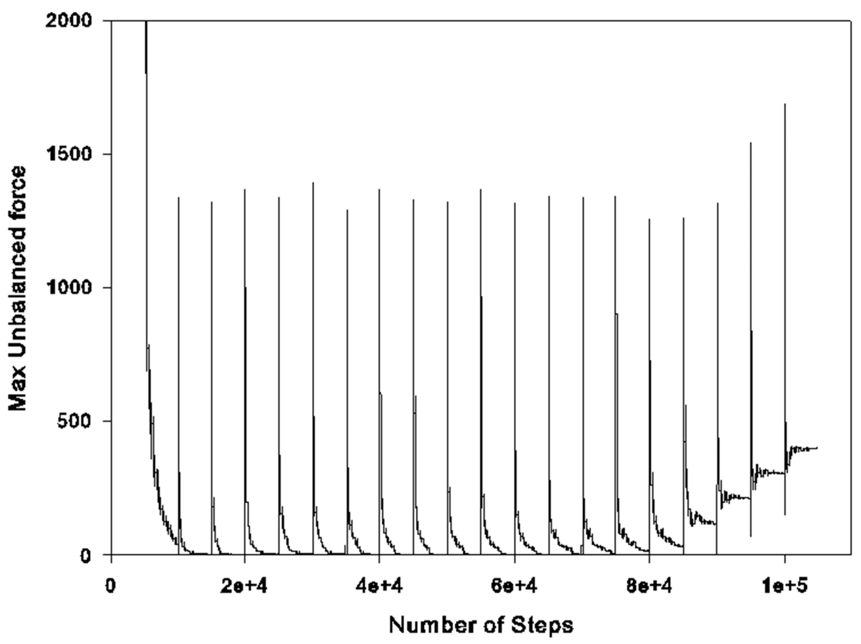
2. Pressure Relaxation Technique

With the development of powerful computers over the last three decades, numerical modelling has proceeded to become a dominant technique for geotechnical problem resolution. The finite difference method is one such technique that is used in this study by using a pressure relaxation method developed for both tunnel stability and settlement problems in this paper. The built-in program language FISH of FLAC is used for this purpose.

Even though tunneling is a complex three-dimensional problem, it can be reasonably simplified to 2D plane strain conditions by taking the transverse section and assuming a very long tunnel that is defined in Figure 2 and Figure 3. The tunnel has a soil overburden C and diameter D. The soil body is modelled as a uniform Tresca material which has both an undrained shear strength (S_u) and unit weight (γ).

A typical finite difference mesh of the problem in this study is shown in Figure 4. The boundary conditions shown in the figure are important as they ensure that the entire soil mass is modelled accurately despite using a finite mesh. It should be noted that the soil domain size for each of the cases was chosen so that the failure zone of the soil body is placed well within the domain. Using Figure 2, L = 2.0 D and W = 8 C are adopted in all analyses of the paper.

After defining boundary conditions, soil properties and tunnel geometry, the developed model “slowly” reduces the internal supporting pressure from the initial at rest condition. In this study, the model was set to fully relax from the starting amount in 1% increments. At each of these relaxation steps (100 steps), the stability number is calculated, and the surface settlement data are recorded. The internal pressure σ_t, is reduced by multiplying the at-rest pressure (where no movement occurs) by a reduction factor, which is based on the specified number of relaxation steps. At each subsequent relaxation step, the internal pressure is less than the at-rest pressure, and consequently the soil moves into the tunnel void until the internal forces in the soil reach equilibrium, balanced or otherwise. In the elastic state, internal forces have reached a balanced state (nodal unbalanced force approaches zero), no more movement takes place, and the circular tunnel is considered as stable. Once the internal pressure is reduced to the extent where the internal forces are no longer sufficient to retain the earth pressures, nodal forces become unbalanced, and the tunnel is unstable.

Note that the failure point occurs when the unbalanced forces fail to reach a zero equilibrium during a particular relaxation stage. This point of instability is the collapse stage and can be identified by observing the unbalanced force history (Figure 5). The appearance of this point is quite abrupt and is determined relatively easily. It can also be observed using plasticity indicator and velocity plots (Figure 6).

The above-mentioned process has been coded using a FISH language, and it was used throughout the paper to perform parametric studies for both stability and settlement responses. Note that all numerical results presented are for dimensionless parameters and therefore their actual values are not important. The followings will discuss the numerical results so obtained.

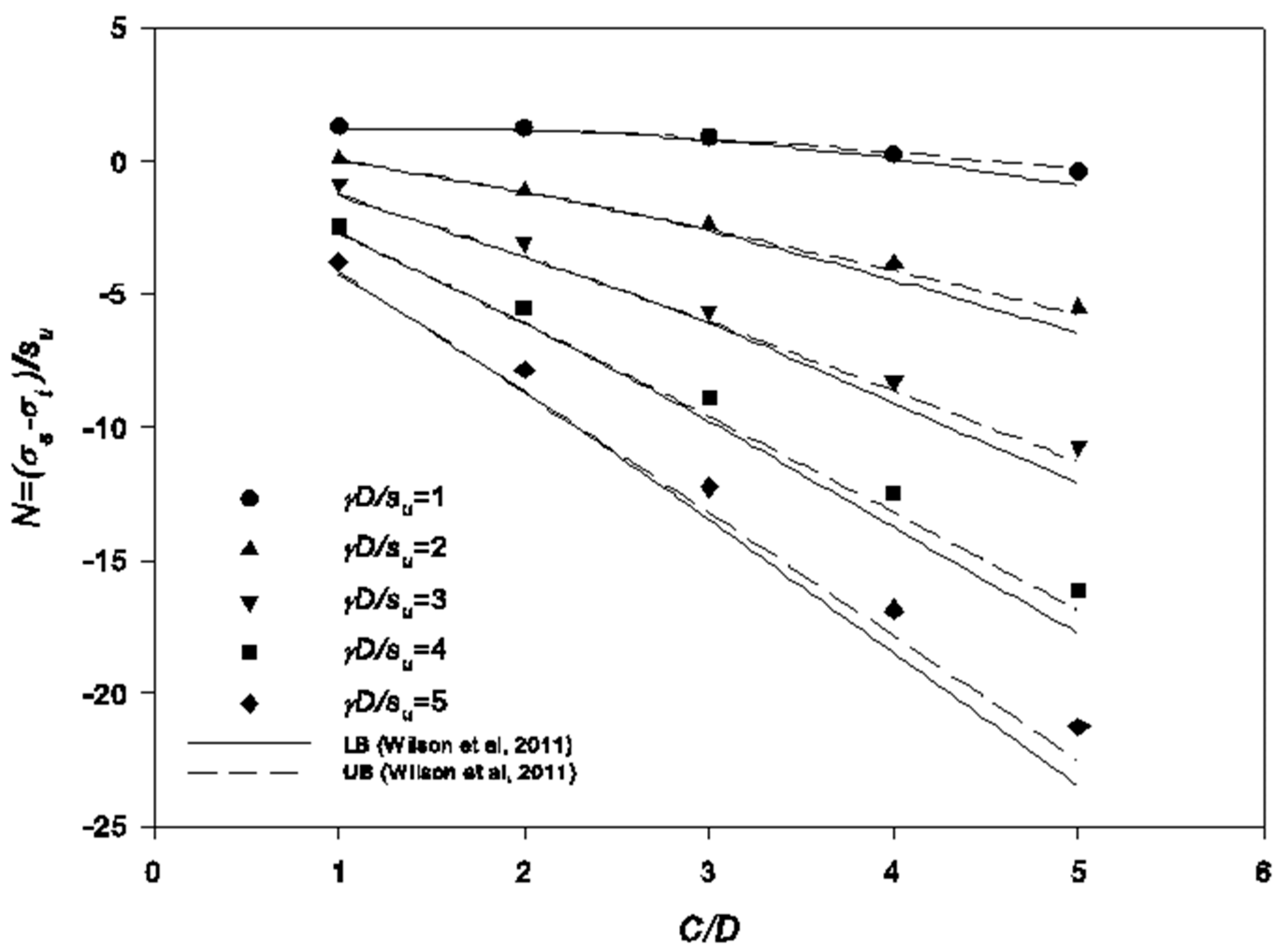
3. Stability Results

Using this internal pressure relaxation method, and a small relaxation interval (amount relaxed each step), the stability number (Equation (2)) that induces collapse can be calculated with reasonable accuracy. It should be noted that the pressure relaxation method will always slightly overestimate the stability number at collapse, as the internal pressure is reduced in discrete steps, not continuously. The internal pressure at the ‘collapse stage’ will have been relaxed slightly more than needed, unless the internal pressure at that stage coincides exactly with the actual collapse stability number.

Figure 7 shows a graphical comparison of stability numbers (N) at collapse using the pressure relaxation method and the rigorous upper and lower bounds. In general, the finite difference results using the pressure relaxation method are in good agreement with FELA solutions [12]. It should be noted that the positive values of stability number, such as those with γD/S_u = 1 for C/D = 1, 2, and 3 suggest that the tunnel would require a negative internal pressure σ_t (or a pulling pressure) to reach the point of imminent collapse. Theoretically, it is considered to be stable and requires no internal pressure to maintain stability. As γD/S_u increase (decrease in soil strength), negative values of stability number are obtained. From the equation (σ_s − σ_t)/S_u, it is known that for a negative stability number, the value of σ_t must be positive, i.e., a positive ‘pushing’ pressure is required to prevent imminent collapse.

Note that, given a constant value of γD/S_u, the stability number (N) decreases with increasing C/D. It can also be seen that, for a constant C/D, the stability number N decreases with increasing strength ratio γD/S_u. These results indicate that greater internal pressure control would be needed for larger value of depth ratio C/D and larger values of strength ratio γD/S_u (softer soils).

A design chart, shown in Figure 8, has been produced. Given values of strength ratio (γD/S_u) and depth ratio (C/D), users can easily identify the critical stability number N = (σ_s – σ_t)/S_u for their design purposes. This can be useful, as it describes the collapse bound, where a hypothetical factor of safety would be one. A surface regression of these data is given in Equation (9), which represents these data with an r² = 0.99:

$$N_c=3-{\left(\frac{C}{D}\right)}^{1.15}{\left(\frac{\gamma D}{s_u}\right)}^{0.82}$$

(9)

The following examples are used to demonstrate the potential of this chart in design and analysis scenarios.

3.1. Practical Example 1—Stability in Soft Soil

A tunnel boring machine has a diameter (D) of 6.0 m and is buried at a depth of 18 m (C) in an undrained clayey material with soil properties S_u = 27 kPa, φ_u = 0°, and γ = 18 kN/m³. The site is assumed to be no surface pressure (σ_s = 0). The following procedures can be used to determine the minimum tunnel internal pressure (σ_t) to prevent collapse.

• Calculate dimensionless ratios from the known data. C/D = 3 and γD/S_u = 4.
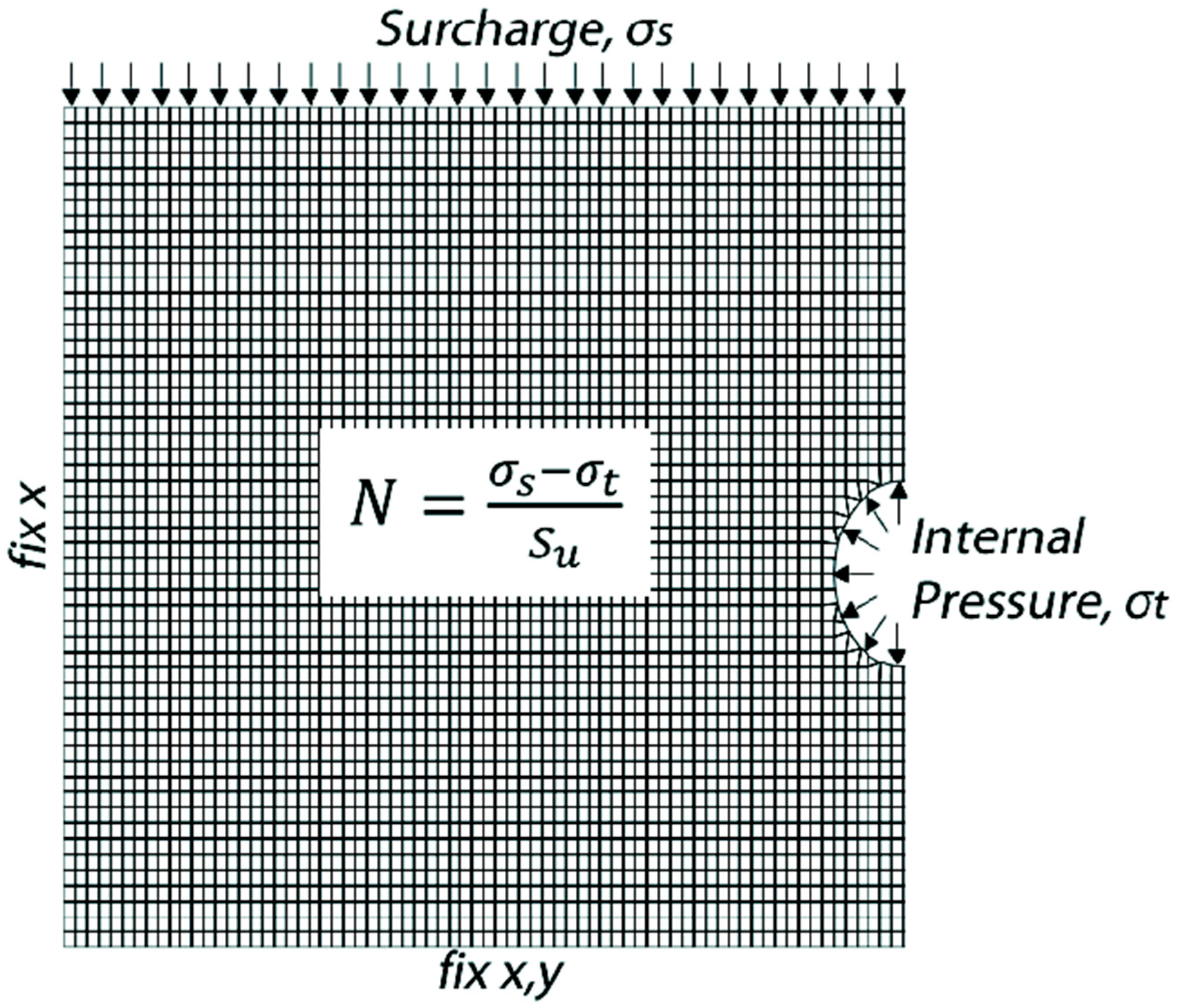
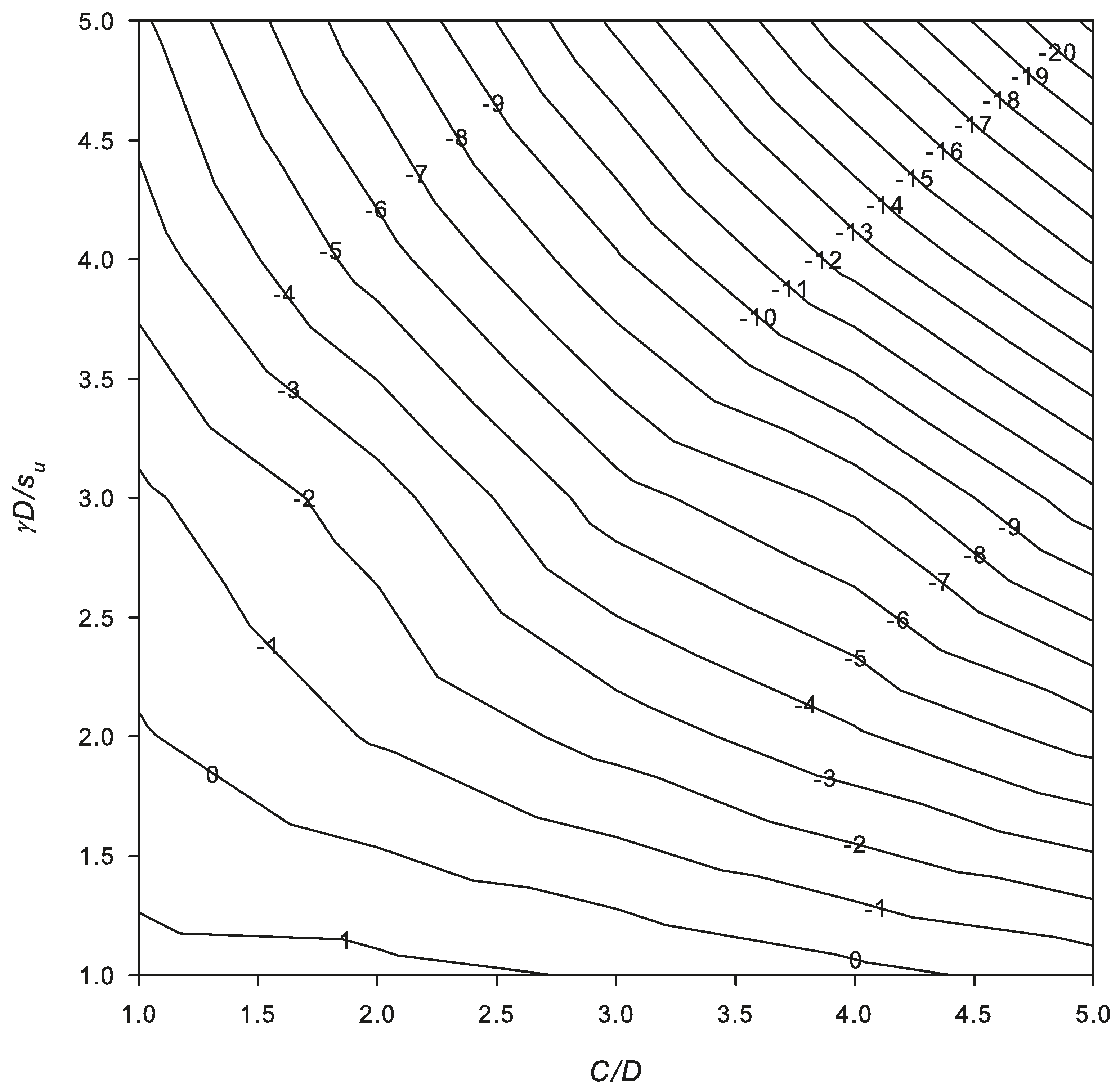
• For a 2D circular tunnel problem with C/D = 3 and γD/S_u = 4.0, Figure 8 returns a value of N = –8.1. Equation (9) yields approximately −8.03 for the same problem.
• Using Equation (2) (N = (σ_s − σ_t)/S_u), σ_t can then be computed as σ_t ≈ 0 − (−8.1 × 27) = 219 kPa. A positive value of σ_t indicates that an internal pushing pressure is required to maintain tunnel stability.

3.2. Practical Example 2—Stability in Stiff Soil

Following Practical Example 1, if we assume that a tunnel boring machine has a diameter (D) of 6.0 m and is buried at a depth of 12 m (C) in an undrained clayey material with properties S_u = 80 kPa, φ_u = 0°, and γ = 18 kN/m³, the following procedures can be used to determine the minimum tunnel internal pressure (σ_t) to maintain the tunnel stability.

• Calculate dimensionless ratios from the known data. C/D = 2 and γD/S_u = 1.35.
• Figure 8 returns a value of N = 0.50.
• Using Equation (2) (N = (σ_s − σ_t)/S_u), σ_t can then be computed as σ_t ≈ 0 − (0.5 × 80) = −40 kPa. A negative value of σ_t such as this indicates that the tunnel requires a pulling pressure to reach a collapse state. In other words, the tunnel will remain stable without any internal pressure.

3.3. Practical Example 3—Depth Determination

A 6 m tunnel is proposed in soil with an undrained clayey material with properties S_u = 40 kPa and γ = 18 kN/m³. If the proposed TBM has the capacity to provide an internal pressure (σ_t) of 300 kPa, and the surface surcharge pressure (σ_s) is found to be 100 kPa, the maximum allowable depth can be back-calculated using Figure 8 and Equation (9).

• Calculate dimensionless ratios from the known data. N = (σ_s − σ_t)/S_u = −5.0 and γD/S_u = 2.7.
• Using Figure 8 and these parameters, the maximum allowable depth ratio (C/D) is approximately 3.1. With a specified tunnel diameter of 6 m, this results in a maximum depth of 18.6 m. If the tunnel is placed any deeper than this, a collapse will be induced. Using Equation (9), a C/D value of 3.0 is obtained.

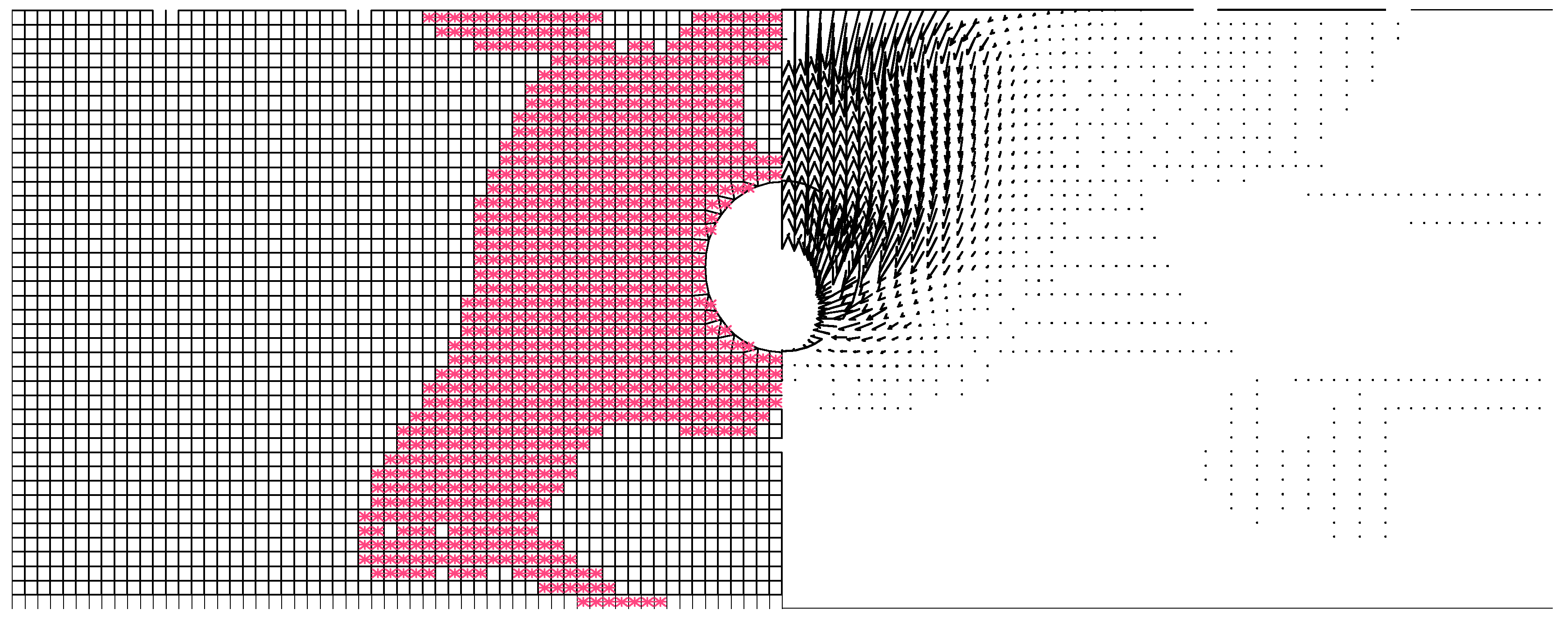
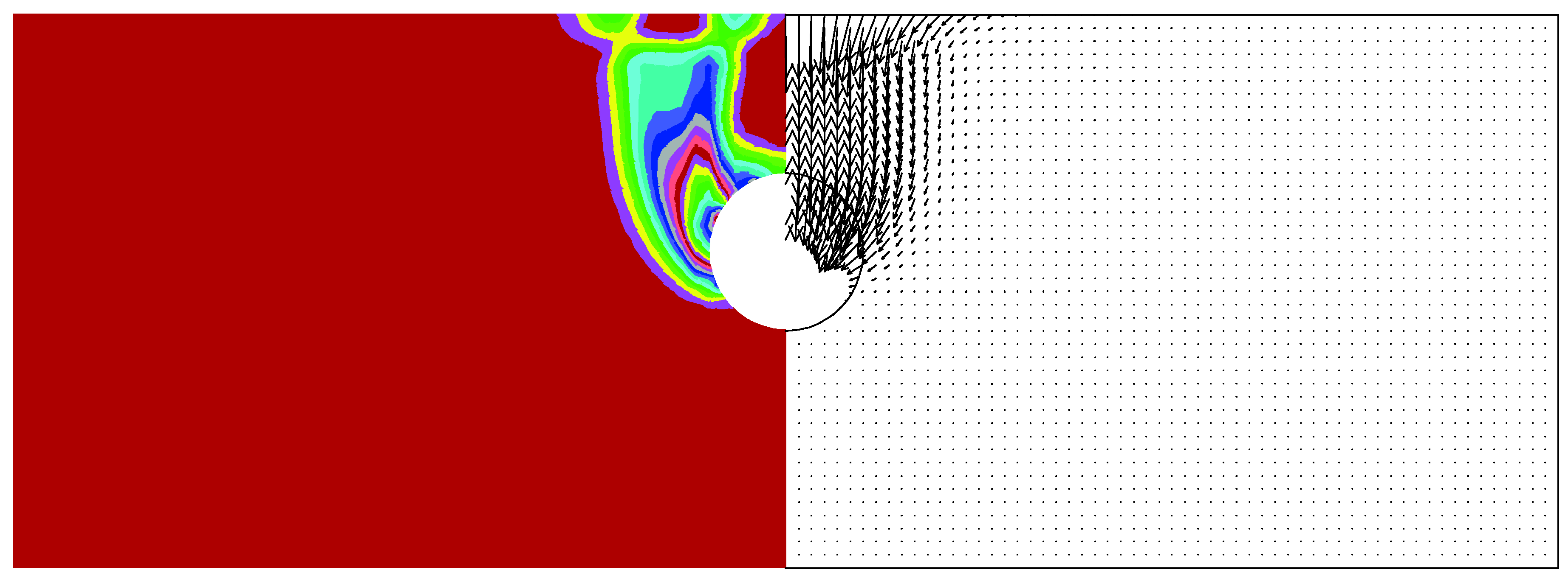
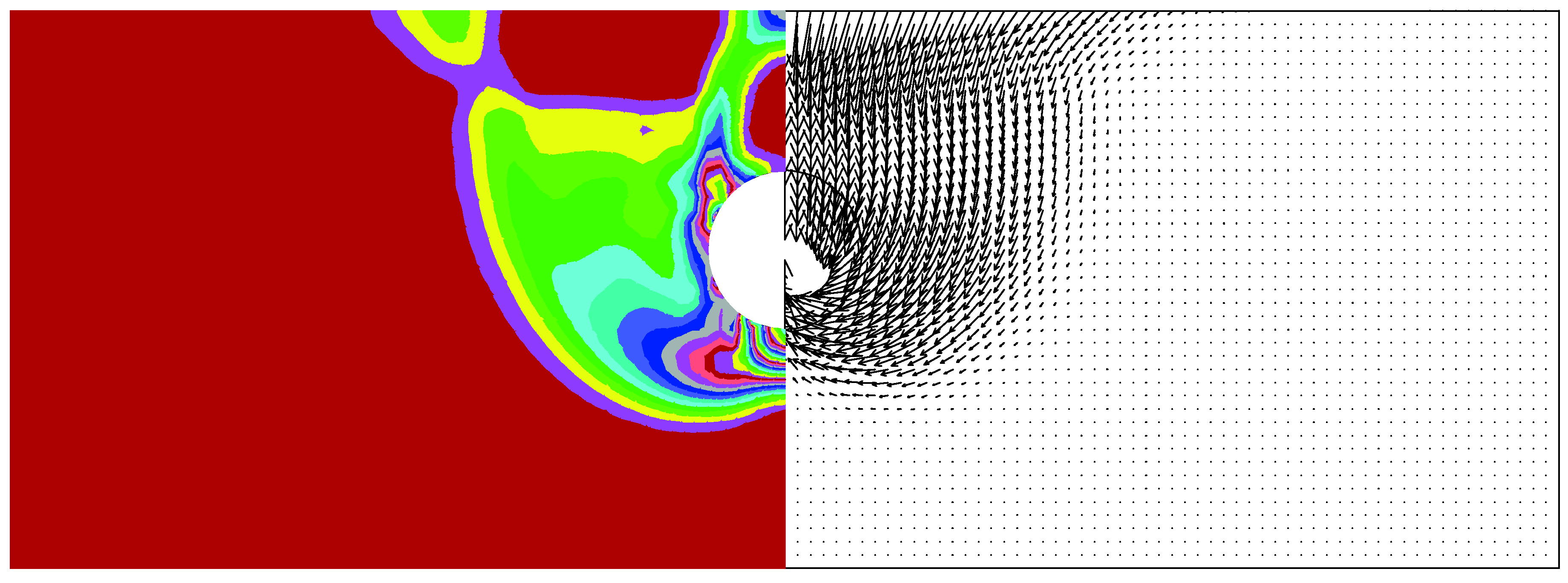
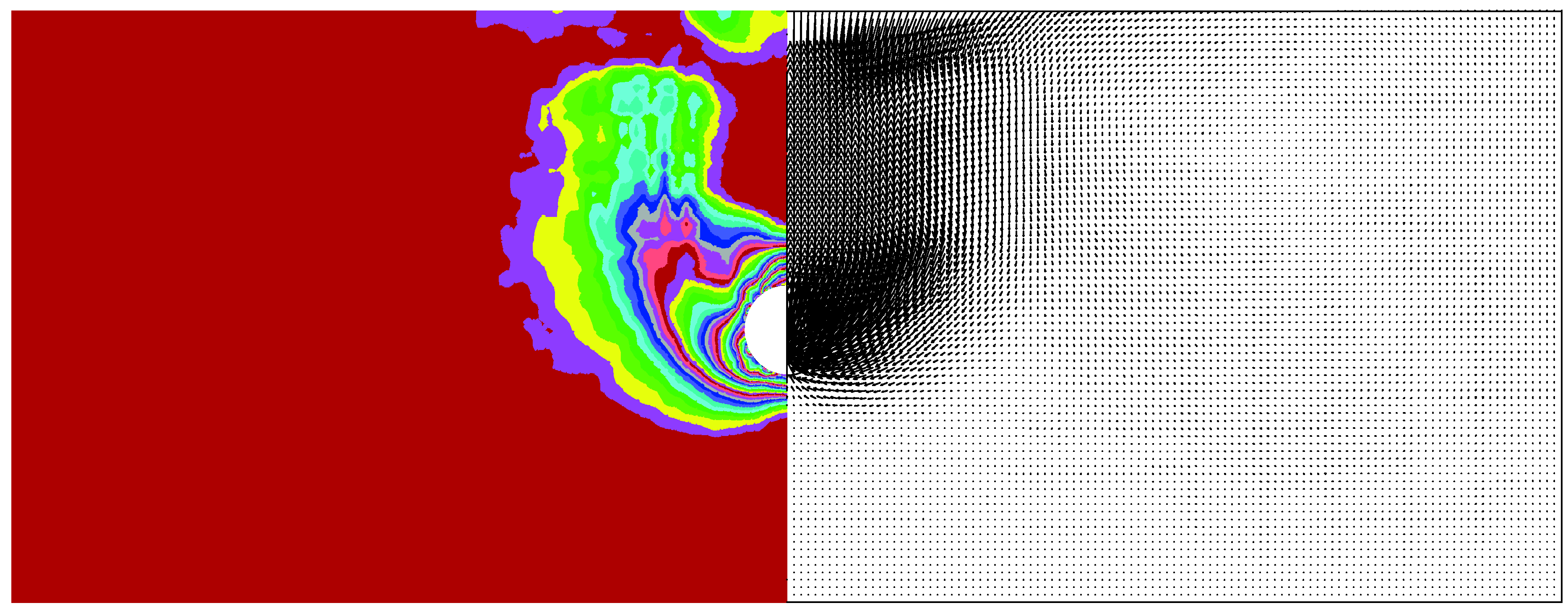
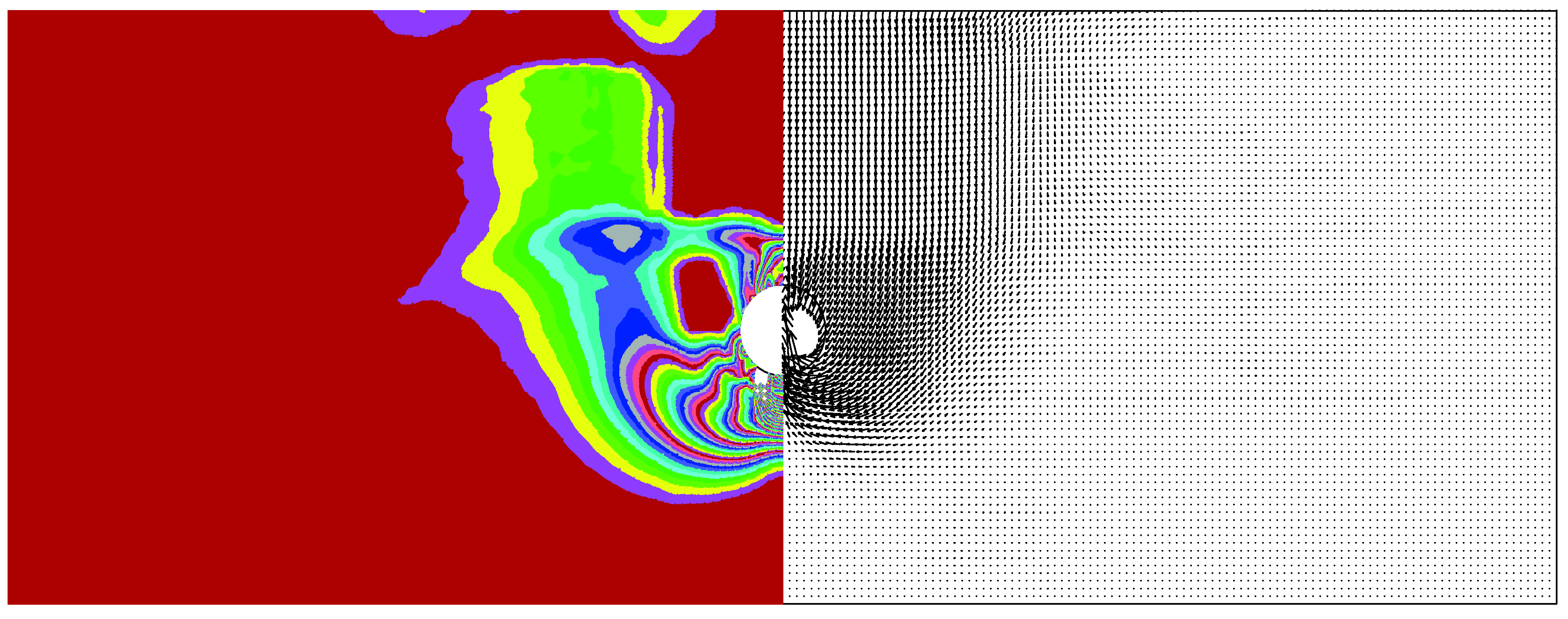
4. Failure Mechanism

Shear strain rate (SSR) plots can be useful to give an indication of failure mechanism, in spite that the actual values are not important in such a perfectly plastic soil modem, and these values are not normally shown in any technical paper. Moreover, due to the space limit, we have selected Figure 9, Figure 10, Figure 11 and Figure 12, showing SSR plots for C/D = 1 and 3, each with γD/S_u = 1 and 5. For all C/D, the failure zone gets wider as the soil strength decreases. Floor heaving is most severe for the deep, soft cases, but reduces for shallow and strong cases. At the surface of all cases, two ‘arms’ are visible with an elastic zone in between. A similar observation is presented in the power dissipation charts by Wilson et al. (2011) [12].

5. Settlement Results

Once the collapse stage has been identified, the surface settlement data can be extracted for that stage. A sample of these settlement profiles are shown in Figure 13, Figure 14, Figure 15 and Figure 16 for various cases, as labeled. As previously discussed, these settlement profiles are commonly represented by the Gaussian equation (see Equation (3)), which has been used for a regression with the data collected at the collapse stage of each of the cases. This has been conducted by using the curve fitting toolbox in MATLAB. A typical example of this is shown in Figure 13. It was found that using this equation to model settlement can be considered as very accurate, with r² values of greater than 0.97 achieved for all cases, where an r² of 1 would indicate a perfect fit. The example shown in Figure 13 is for C/D = 4, γD/S_u = 3, and this example has an r² = 0.987.

In Figure 14, the depth ratio (C/D) is varied, and the strength ratio (γD/S_u) and Young’s modulus (E) are kept constant. The shallow case produces a narrow but deep trough, and it then becomes shallower and wider as C/D increases. In Figure 15, C/D and E are kept constant, and γD/S_u is varied. Once again, the trend is as expected, when the strength ratio is increased (i.e., soils become weaker), the settlement at the point of collapse is greater. Figure 16 similarly shows the impact of Young’s modulus, with the stiffer soils (higher E) having proportionately lower settlement.

The i_x values can be produced for each case reliably by using Equations (3) and (4) for the obtained numerical data. With i_x values obtained for the collapse stage, some observations can be made regarding the impact of the Young’s modulus parameter (E). From Figure 16, it is noted that this parameter E has significant effect on volume loss. However, in Figure 17 and Figure 18, the two graphs show that E has little to no impact on the i_x value so obtained.

With this established, the complete results can be presented with less confusion. Figure 19 is a graph showing the dimensionless trough parameter (i_x/D) against H/D with various γD/S_u. Presenting the results in this way allows them to be examined using O’Reilly and New’s (1982) [23] relationship, as in Equation (8). From this relationship, the proportionality constant (k) can be calculated for each case. As can be seen from the figure, the k values can be estimated reasonably based solely on γD/S_u. Figure 20 shows this relationship; a linear regression can be applied to give a convenient expression for estimating k, and by extension the value of i_x. This is given in Equation (10):

$$k=\frac{i_x}{H}=0.05\frac{\gamma D}{S_u}+0.52$$

(10)

Mair and Taylor (1997) [20] supported a recommendation that a k of 0.5 could be reasonably selected for undrained clay. This equation would tend to support this, and in strong clays it will approach 0.52 (see Equation (10)).

Figure 21 shows the results of the regression in this study, as compared to suggested equations for i_x as listed in Equations (5)–(7). Note that Equation (5) is based on γD/S_u ≈ 1.8 (Clough and Schmidt, 1981 [25]), Equation (6) is based on γD/S_u ≈ 2.6 (Mair and Taylor, 1997 [20]), and Equation (7) is based on γD/S_u ≈ 3 (Lee et al. 1999 [26]). It can be understood that the results from this study do not match particularly well with these equations. This is due to the estimates in this study being based on the collapse stage where the volume loss is much higher. The equations are based off data where the tunnel was closer to working condition’s volume loss. If the settlement data were exported at an earlier relaxation stage (i.e., lower simulated volume loss), lower i_x values would be expected (Palmer and Mair, 2011) [28].

6. Conclusions

A numerical procedure has been developed for analyzing tunnels based on a pressure relaxation method that simulates the relaxation of the soil around the excavation and the grout pressure behind the lining. This model is robust, and it allows parametric analyses to be performed efficiently and effectively. This study has carried such an analysis on circular tunnels in undrained clay, over a practical range of dimensionless ratios: C/D, γD/S_u, and E/S_u. Both stability and settlement have been analyzed and reported, with a particular focus on the stage of collapse. The following conclusions are drawn based on the current study.

• Validation of the model shows that promising results are obtained using the developed model. Comparison with rigorous upper and lower bound results shows that the results using current pressure relaxation method are accurate and can be used with confidence as a design tool in practice. Based on the parametric study, a design chart is developed, and several practical examples are shown on how to use the design chart.
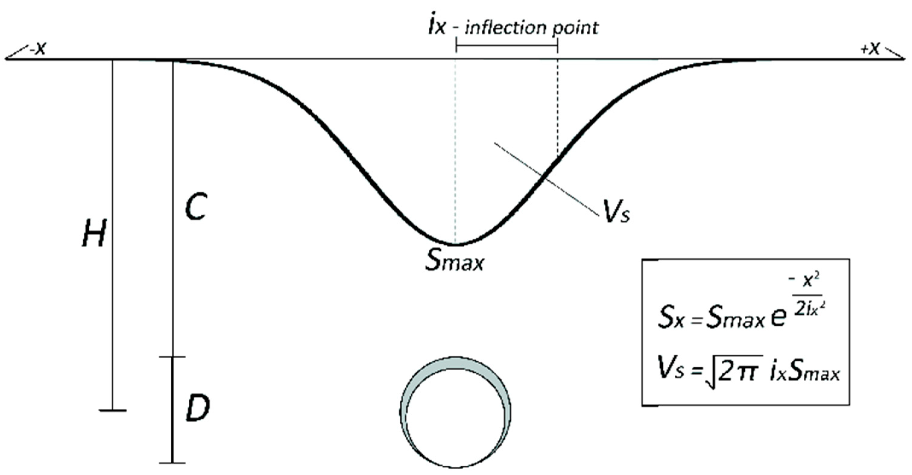
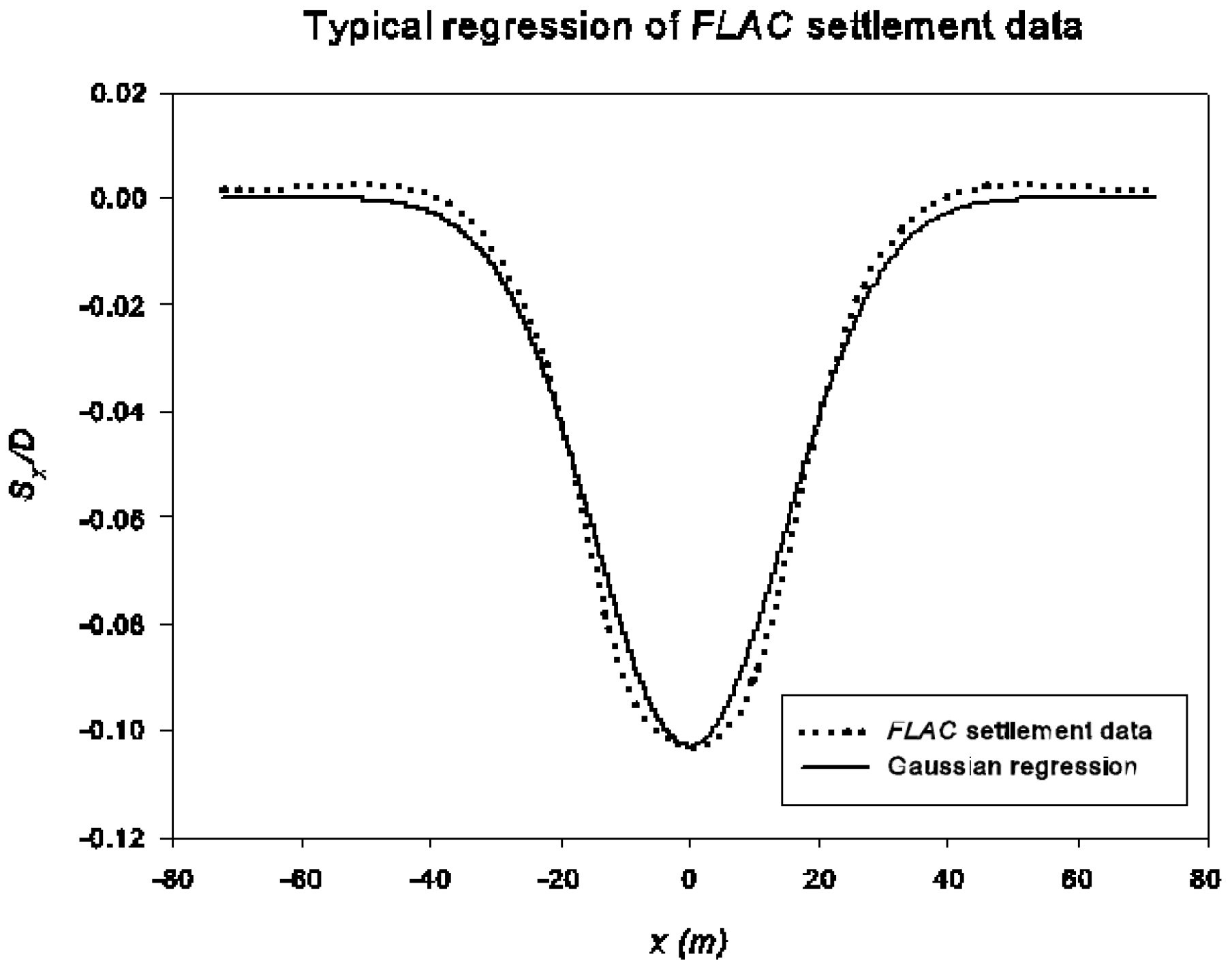
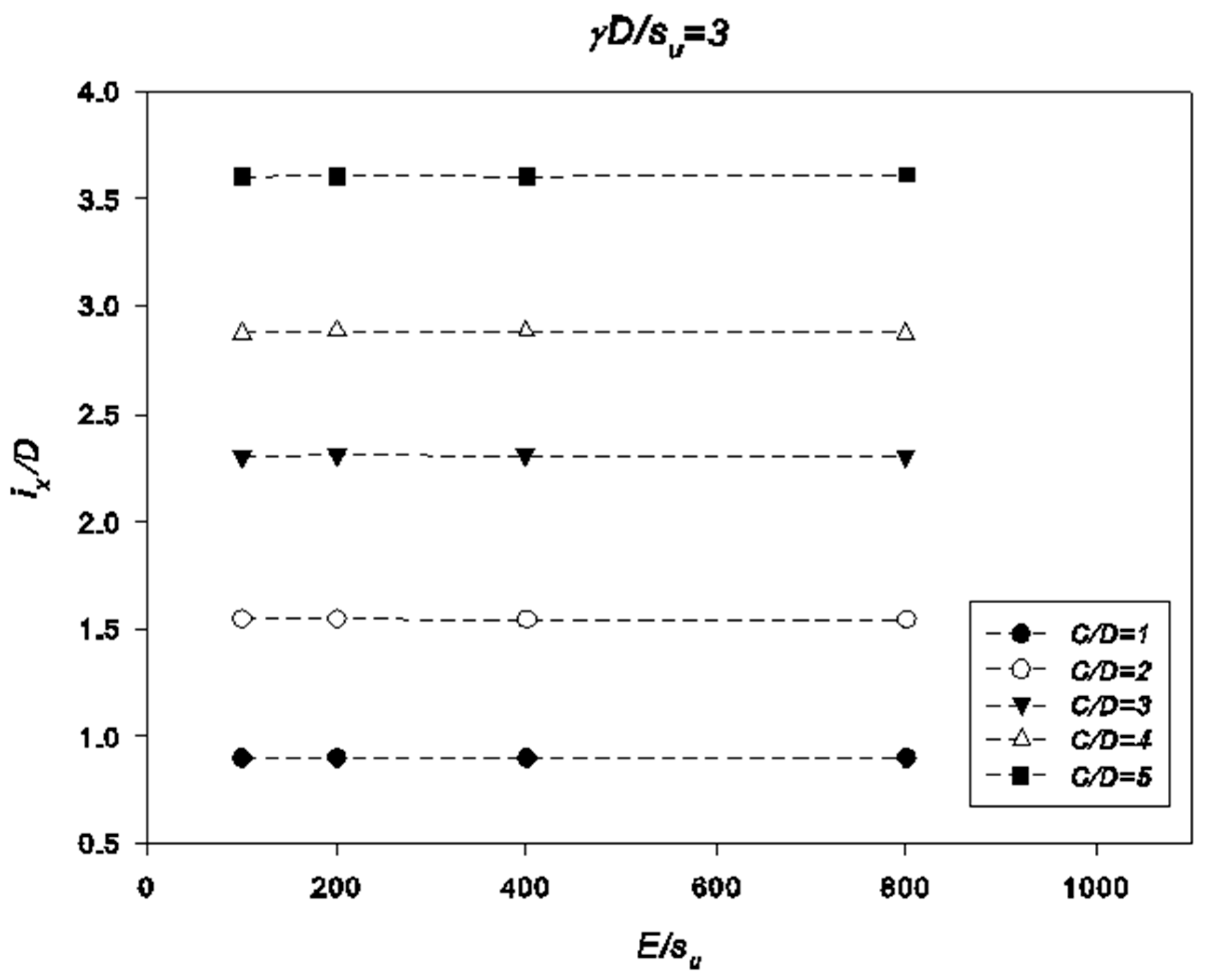
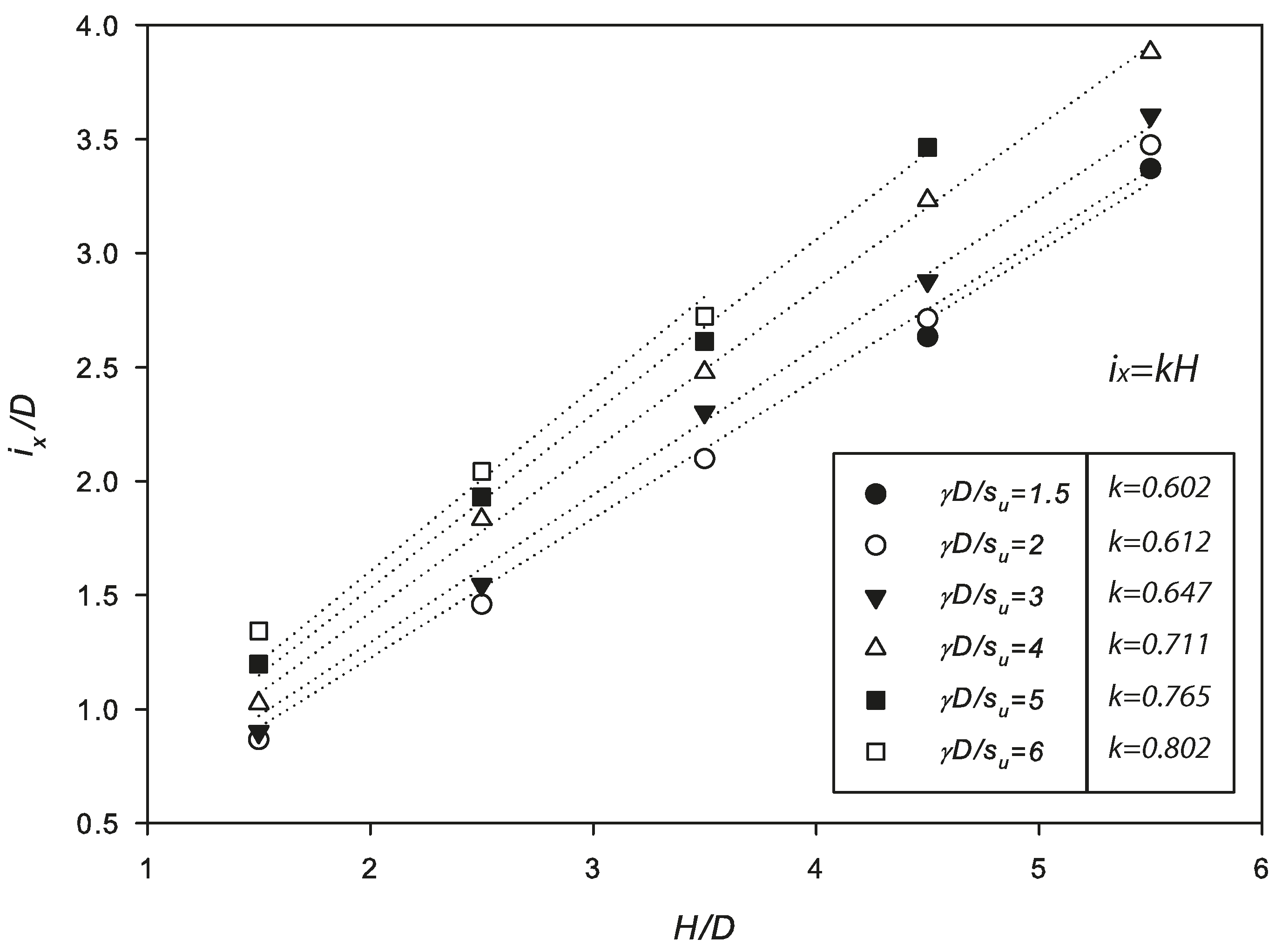
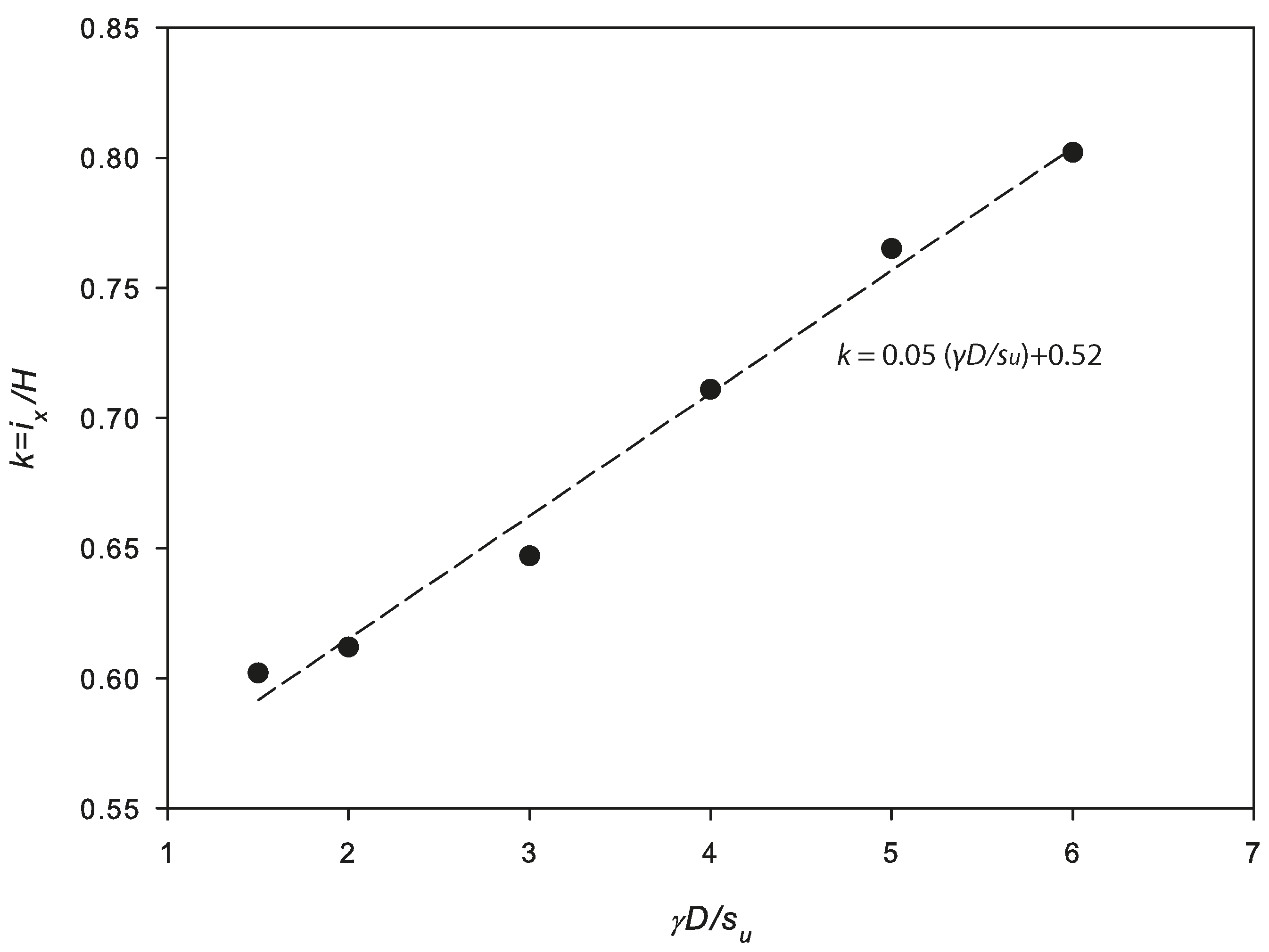
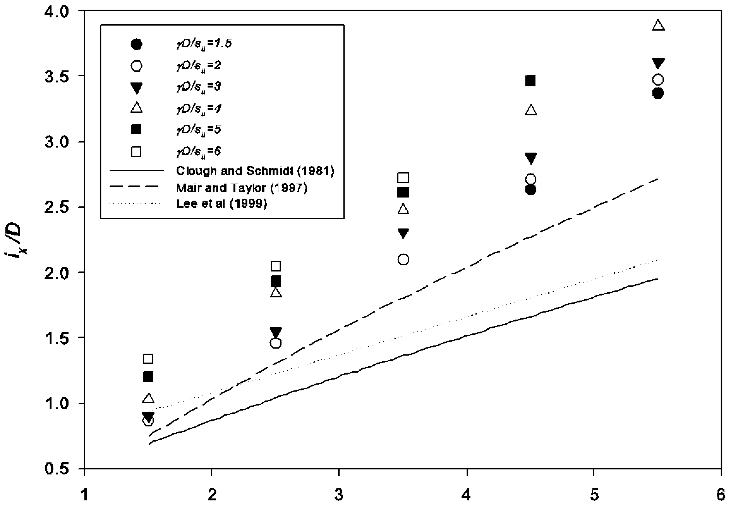
• The great similarity between the obtained settlement and the Gaussian curve indicates that this empirical method is still suitable to be applied in the industry as a preliminary tool. This research suggests that the constant k should be approximately between 0.55–0.75 for undrained clays. A new equation is proposed for estimating the k value based on a linear regression analysis.
• Using a Gaussian distribution curve requires an estimation of S_max, which would likely be estimated by using a volume loss limit. Work in the future needs to be able to estimate k accurately at lower levels of relaxation and with lower volume loss.
• It was concluded that this automated process has many practical significances for industry application. Future work can be attributed to underground mining application.

References

1. Peck, R.B. Deep excavations and tunneling in soft ground. In Proceedings of the 7th International Conference on Soil Mechanics and Foundation Engineering, Held in Mexico City, 1969; Sociedad Mexicana de Mecanica: Mexico City, Mexico; Volume 4, pp. 225–290.
2. Broms, B.B.; Bennermark, H. Stability of clay at vertical openings. J. Soil Mech. Found. Div. 1967, 193, 71–94. [Google Scholar] [CrossRef]
3. Mair, R.J. Centrifugal Modelling of Tunnel Construction in Soft Clay. Ph.D. Thesis, University of Cambridge, Cambridge, UK, 1979. [Google Scholar]
4. Davis, E.; Gunn, M.; Mair, R.; Seneviratine, H. The stability of shallow tunnels and underground openings in cohesive material. Geotechnique 1980, 30, 397–416. [Google Scholar] [CrossRef]
5. Shiau, J.S.; Lyamin, A.V.; Sloan, S.W. Rigorous solutions of classical lateral earth pressures. In Proceedings of the 6th Australia–New Zealand Young Geotechnical Professionals Conference, Gold Coast, Australia, December 2003; pp. 162–167. [Google Scholar]
6. Shiau, J.S.; Lyamin, A.V.; Sloan, S.W. Application of pseudo-static limit analysis in geotechnical earthquake design. In Numerical Methods in Geotechnical Engineering; Schweiger, Ed.; Taylor & Francis Group: London, UK, 2006; pp. 249–255. [Google Scholar]
7. Shiau, J.; Al-Asadi, F. Three-dimensional heading stability of twin circular tunnels. Geotech. Geol. Eng. 2020, 38, 2973–2988. [Google Scholar] [CrossRef]
8. Shiau, J.; Al-Asadi, F. Stability analysis of twin circular tunnels using shear strength reduction method. Géotech. Lett. 2020, 10, 311–319. [Google Scholar] [CrossRef]
9. Shiau, J.; Al-Asadi, F. Twin tunnels stability factors Fc, Fs and Fγ. Geotech. Geol. Eng. 2021, 39, 335–345. [Google Scholar] [CrossRef]
10. Shiau, J.; Al-Asadi, F. Revisiting circular tunnel stability using Broms and Bennermarks’ Original Stability Number. Int. J. Geomech. 2021, 21, 06021009. [Google Scholar] [CrossRef]
11. Sloan, S. Geotechnical stability analysis. Geotechnique 2013, 63, 531–571. [Google Scholar] [CrossRef] [Green Version]
12. Wilson, D.W.; Abbo, A.J.; Sloan, S.W.; Lyamin, A.V. Undrained stability of a circular tunnel where the shear strength increases linearly with depth. Can. Geotech. J. 2011, 48, 1328–1342. [Google Scholar] [CrossRef]
13. Loganathan, N.; Poulos, H.G. Analytical prediction for tunneling-induced ground movements in clays. J. Geotech. Geoenviron. Eng. 1998, 124, 846. [Google Scholar] [CrossRef]
14. Rankin, W. Ground movements resulting from urban tunnelling: Predictions and effects. Geol. Soc. Lond. Eng. Geol. Spec. Publ. 1988, 5, 79–92. [Google Scholar] [CrossRef]
15. Sagaseta, C. Analysis of undraind soil deformation due to ground loss. Geotechnique 1987, 37, 301–320. [Google Scholar] [CrossRef]
16. Gunn, M.J. The prediction of surface settlement profiles due to tunneling. In Predictive Soil Mechanics, Proceedings of the Wroth Memorial Symposium, St. Catherines College, Oxford, UK, 27–29 July 1992; Thomas Telford Publishing: London, UK, 1992. [Google Scholar]
17. Taylor, R. Modelling of tunnel behaviour. Proc. ICE-Geotech. Eng. 1998, 131, 127–132. [Google Scholar] [CrossRef]
18. Martos, F. Concerning an approximate equation of the subsidence trough and its time factors. In Proceedings of the International Strata Control Congress, Leipzig, Germany, 14–16 October 1958; pp. 191–205. [Google Scholar]
19. Atkinson, J.; Cairncross, A. Collapse of a shallow tunnel in a Mohr-Coulomb material. In Proceedings of the Symposium on the Role of Plasticity in Soil Mechanics, Cambridge, UK, 13–15 September 1973. [Google Scholar]
20. Mair, R.J.; Taylor, R.N. Theme lecture: Bored tunnelling in the urban environment. In Proceedings of the 14th International Conference on Soil Mechanics and Foundation Engineering, Hamburg, Germany, 6–12 September 1997; pp. 2353–2385. [Google Scholar]
21. Attewell, P.; Farmer, I. Ground deformations resulting from shield tunnelling in London Clay. Can. Geotech. J. 1974, 11, 380–395. [Google Scholar] [CrossRef]
22. Cording, E.J.; Hansmire, W.H. Displacement around soft ground tunnels—General report. In Proceedings of the 5th Pan-American Conference on Soil Mechanics and Foundation Engineering, Buenos Aires, Argentina, 15–19 November 1975. [Google Scholar]
23. O’Reilly, M.P.; New, B.M. Settlements above tunnels in the United Kingdom—Their magnitude and prediction. Tunneling 1982, 82, 173–181. [Google Scholar] [CrossRef]
24. Phienwej, N. Ground movements in shield tunneling in Bangkok soils. In Proceedings of the 14th International Conference on Soil Mechanics and Foundation Engineering, Hamburg, Germany, 6–12 September 1997; Volume 3, pp. 1469–1472. [Google Scholar]
25. Clough, G.W.; Schmidt, B. Design and performance of excavations and tunnels in soft clay. In Soft Clay Engineering; Elsevier: Amsterdam, The Netherlands, 1977; pp. 569–634. [Google Scholar]
26. Lee, C.J.; Wu, B.R.; Chiou, S.Y. Soil movements around a tunnel in soft soils. Proc. Natl. Sci. Counc. Part A Phys. Sci. Eng. 1999, 23, 235–247. [Google Scholar]
27. Guglielmetti, V.; Grasso, P.; Mahtab, A.; Xu, S. (Eds.) Mechanized Tunnelling in Urban Areas: Design Methodology and Construction Control; Taylor and Francis: Abingdon, UK, 2008; Chapter 5. [Google Scholar]
28. Palmer, A.C.; Mair, R.J. Ground movements above tunnels: A method for calculating volume loss. Can. Geotech. J. 2011, 48, 451–457. [Google Scholar] [CrossRef]
Figure 1. Schematic diagram of a TBM indicating overcutting (not to scale).
Geosciences 13 00081 g001
Figure 2. Problem definition.
Geosciences 13 00081 g002
Figure 3. Typical tunnel settlement problem.
Geosciences 13 00081 g003
Figure 4. Typical mesh of the problem.
Geosciences 13 00081 g004
Figure 5. Unbalanced force history plot (C/D = 3, γD/Su = 4, E = 200 Su).
Geosciences 13 00081 g005
Figure 6. Plasticity (left), and velocity (right) plots at the stage of collapse (C/D = 1, γD/Su = 3).
Geosciences 13 00081 g006
Figure 7. Comparison of critical stability numbers from this study with rigorous upper and lower bounds from Wilson et al. (2011).
Geosciences 13 00081 g007
Figure 8. Contour plot of critical stability numbers, N = (σs − σt)/Su, obtained from this study.
Geosciences 13 00081 g008
Figure 9. Shear strain rate (SSR) and velocity plot for C/D = 1, γD/Su = 1.
Geosciences 13 00081 g009
Figure 10. Shear strain rate (SSR) and velocity plot for C/D = 1, γD/Su = 5.
Geosciences 13 00081 g010
Figure 11. Shear strain rate (SSR) and velocity plot for C/D = 3, γD/Su = 1.
Geosciences 13 00081 g011
Figure 12. Shear strain rate (SSR) and velocity plot for C/D = 3, γD/Su = 5.
Geosciences 13 00081 g012
Figure 13. A typical regression of the Gaussian equation to the FLAC data.
Geosciences 13 00081 g013
Figure 14. Typical settlement profiles with respect to C/D (depth ratio).
Geosciences 13 00081 g014
Figure 15. Typical settlement profiles with respect to γD/Su (soil strength ratio).
Geosciences 13 00081 g015
Figure 16. Typical settlement profiles with respect to E/Su (Young’s modulus ratio).
Geosciences 13 00081 g016
Figure 17. Young’s modulus against ix with respect to γD/Su.
Geosciences 13 00081 g017
Figure 18. Young’s modulus against ix with respect to C/D.
Geosciences 13 00081 g018
Figure 19. Complete results of regression analysis, and resulting proportionality constants (k).
Geosciences 13 00081 g019
Figure 20. Relationship between k and γD/Su.
Geosciences 13 00081 g020
Figure 21. Comparison of results with other suggested equations.
Geosciences 13 00081 g021
Disclaimer/Publisher’s Note: The statements, opinions and data contained in all publications are solely those of the individual author(s) and contributor(s) and not of MDPI and/or the editor(s). MDPI and/or the editor(s) disclaim responsibility for any injury to people or property resulting from any ideas, methods, instructions or products referred to in the content.