
FEM Modelling of Thin Weak Layers in Slope Stability Analysis


Department of Chemistry, Life Sciences and Environmental Sustainability, University of Parma, 43124 Parma, Italy
Geosciences 2023, 13(8), 233; https://doi.org/10.3390/geosciences13080233
Submission received: 25 June 2023
/
Revised: 18 July 2023
/
Accepted: 4 August 2023
/
Published: 6 August 2023
(This article belongs to the Special Issue Advanced Numerical Modelling and Analysis in Geotechnical Engineering)
Abstract
:Modelling the presence and the effect of a thin weak layer of soil or rock in a slope stability analysis performed through the finite element method (FEM) presents several problems of purely numerical nature. This paper deals with a parametric analysis of three different 2D numerical case studies (both ideal and real) of unstable or potentially unstable slopes containing a thin soft band (or weak layer). The FEM software used is RS2 (Rocscience®). The aim is investigating the influence of some geometrical and numerical characteristics of the soft bands in the stability analyses. The Mohr–Coulomb elastic-perfectly plastic constitutive model for all the involved materials was assumed, and the mechanical parameters were kept constant. Instead, other fundamental parameters of the weak layer, such as the type of mesh elements, the mesh density, and the geometry, in terms of both thickness and outcrop shape, were changed, and results in terms of the critical Strength Reduction Factor (SRF) were compared. The main outcomes of this study represent practical suggestions on some numerical and technical aspects to users of FEM slope stability analyses, in order to obtain a precautionary assessment of slope stability.
1. Introduction
Numerical modelling of thin weak layers or soft bands in slope stability analysis has long been a subject of study, and the available scientific literature on this topic is very broad [1,2,3,4,5,6,7,8,9]. It is reasonable that the presence of a thin shear band or a weak layer in a slope can be considered effectively modelled by means of a sliding surface, which corresponds to the basic assumption of the limit equilibrium method (LEM). On the other hand, it is well known that the presence of a thin weak layer in a slope could be appropriately modelled using a discontinuous approach. Some authors investigated the initiation and progressive failure in a natural rock slope by using both continuum (finite-element) and hybrid (finite-/discrete-element). They showed that the failure process along a slide plane and internal strength degradation could be effectively modelled numerically [10]. However, if a numerical code based on the Finite Element Method (FEM) and on the Strength Reduction Method (SRM) is adopted, modelling a thin weak layer presents several problems of purely numerical nature. The first practical problem in applying the SRM to a slope with a soft band by using FEM is that when the soft band is very thin, the number of elements required to achieve a good solution is extremely large, so that a very high computational burden and time are required [11].
Comparing 3D and 2D slope failure analyses by LEM and FEM, Wei et al. (2009) investigated the stability of a vertical rock cut with a weak layer [12]. By conducting several stability analyses, they found a good level of agreement comparing LEM and FEM results, although they point out a higher factor of safety (FoS) values in 3D models than in 2D ones. Wei et al. (2009) also noted the influence of the mesh and its characteristics on the modelling of slopes with thin weak layers. Depending on the type of mesh, the number of elements, and the number of nodes in the mesh, there is a variation in the value of FoS, which is an indicator of the global stability conditions. The same authors also pointed out how results are deeply affected by the mesh shape and cell size at the slope toe [12].
Other authors showed as for slopes with a thin soft band, the FoS value obtained using the traditional Lagrangian-based FEM with the convergence criterion is not valid because the non-convergence is due to severe local mesh distortion. To solve this problem, they proposed a slope stability analysis method by incorporating the Coupled Eulerian–Lagrangian (CEL) FEM and the shear strength reduction (SSR) technique [6].
When it is necessary to model the presence of a thin soft band in a slope, an appropriate selection of the adopted numerical parameters and the way in which the numerical model is built become of crucial importance. Weak layers are usually characterised by small thickness and poor mechanical properties. The effective cohesion is often very low, even close to zero. As regards the geometry, it is difficult to identify the weak layer in terms of thickness and spatial continuity, so it is not always well known, although it greatly affects numerical results.
This paper deals with a parametric analysis of three different 2D numerical models of unstable or potentially unstable slopes containing a thin soft band (or weak layer). The commercial FEM software RS2—Rocscience® will be used. The aim is investigating the influence of some characteristics of the soft bands in the stability analyses. It is worth underlining that the parametric analysis will regard only numerical and geometrical parameters; instead, mechanical parameters of the materials will be kept constant.
The models analysed in this paper are divided into two categories: ideal and real models. The ideal models (ID-1 and ID-2) are characterised by geometries and input parameters defined theoretically, which have been collected from the scientific literature [2,12]. Considering those ideal models allows a comparison, in terms of obtained results, with different numerical codes used by other authors. The real model is much more complex and represents the reconstruction of a specific section of the Lemeglio landslide in Northern Italy [13].
The adopted software (RS2—Rocscience®) allows carrying out the SRM until the model reaches the so-called numerical instability, which ideally corresponds to a physical instability, thus defining the critical Strength Reduction Factor (SRF).
The analyses were carried out by assuming the Mohr–Coulomb elastic-perfectly plastic constitutive model for all the materials involved and by varying some fundamental parameters of the weak layer, such as the type of mesh elements, the mesh density, and the geometry, in terms of both thickness and outcrop shape.
2. Materials and Methods
The first ideal model (ID-1) is the same assumed in [2] in terms of both geometry and mechanical properties (Figure 1).
It is characterised by a thin weak layer (WL) with a constant thickness of 0.5 m, which emerges horizontally at the slope toe. The slope is 15 m in height, and the domain has a total length of 28 m. The strength and stiffness parameters of the three layers of the model are reported in Table 1.
The second ideal model (ID-2) is partially similar to that considered in [12], since it is a 2D model instead of the 3D model assumed in [12] (Figure 2). Moreover, instead of assuming a vertical cut (90°), as in [12], the slope is 70° steep. The weak layer (WL) is represented by a planar band, with an inclination of 35° with respect to the horizontal plane. It has a constant thickness of 0.5 m and plunges at the foot of the slope without intersecting the slope surface. The slope is 5 m high, and the domain has a total base length of 10 m. The strength and stiffness parameters for the three layers of the model are reported in Table 1. These parameters have been assumed the same as in the ID-1 model in order to compare results of the two ideal models.
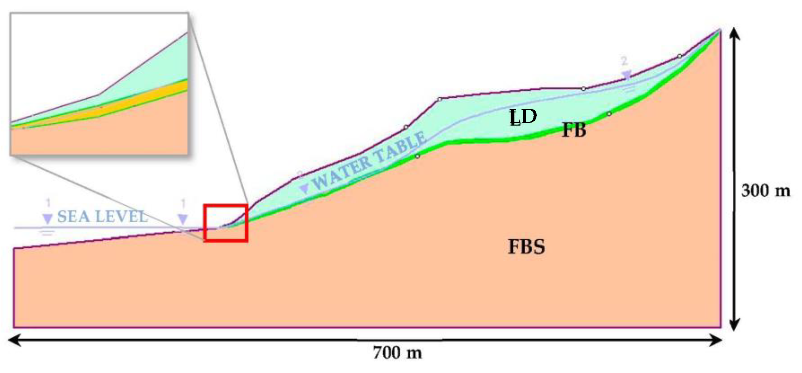
The Lemeglio Landslide Model (LLM) has been reconstructed thanks to the study presented in [13]. As it can be noticed in Figure 3, which represents the slope in the most representative cross-vertical section, the weak layer made by the Friction Breccia has a variable thickness, which can be preliminarily assumed equal to 2 m and constant everywhere. The studied section has a height of about 200 m, starting from the sea level at the foot, and a total length of 700 m. The slope faces directly into the sea, and the water table meets the sea level (Figure 3). The strength and stiffness parameters for the three layers of the model are the same as adopted in [13] and are reported in Table 1. As pointed out in the introduction, all these mechanical parameters will be kept constant in the different numerical analyses.
The first objective of FEM analyses was assessing the effect of the type, number of mesh elements, and number of nodes on the critical SRF.
RS2 code allows defining automatically triangular or quadrilateral mesh elements, with or without intermediate nodes. The generated mesh is characterised by a specific number of elements and by a certain uniformity degree. A specific and interesting aspect consists in the densification of the mesh, only in certain portions of the slope, such as the weak layer, which is normally very thin with respect to the rest of the domain.
The geometry of the weak layers was also varied in order to assess the effect of different thicknesses and positions, i.e., distinguishing the geometry of the outcrop of the weak material along the slope surface.
One of the first objectives was recognising which type of mesh can provide the most reliable (and stable) critical SRF value. This objective has been reached by performing FEM analyses using a uniform mesh on the ID-1 model, as it will be explained in the following (Section 3.1.1). By comparing the obtained results with those reported in [2], the mesh generated using 6-nodes triangular meshes proved to be the most efficient (see Section 3.1.1) and was, therefore, used in the subsequent analyses.
In particular, the following analyses were carried out on the three studied models:
- Analysis with uniform mesh;
- Analysis with intensified mesh in the weak layer;
- Analysis with variable thickness of the weak layer;
- Analysis with variable outcrop geometry of the weak layer.
In all the models analysed, displacements in the horizontal and vertical directions at the base and sides of the calculation domain were prevented, while nodes on the slope surface were left unblocked.
2.1. Analysis with Uniform Mesh
As discussed in the previous section, it should be noted that the mesh can be set according to various types of density. In the analysed models, the uniform mesh was used, i.e., the mesh has a homogeneous distribution of nodes and elements over the entire domain.
To set the uniform mesh, it was necessary to introduce as input an approximate number of elements. It is worth reminding that the number of elements entered when setting up the mesh is an approximate number: the actual number of generated elements can be known after creating the mesh, and it is generally greater than the input number.
The number of elements and nodes in the mesh was an interesting parameter to be studied: for each model, analyses were carried out by gradually increasing the number of elements and nodes in the uniform mesh.
However, since each model presents unique geometric characteristics, it was not possible to replicate the same set of elements and nodes. Different analyses were performed with a number of elements in the range between 1500 and 10,000. As expected, the computational time strongly increased by increasing the number of elements in the mesh.
It is also interesting considering the way in which RS2 software creates the mesh in some specific areas, where the geometric characteristics tend to be particular: reference is obviously made to the weak layer, whose thickness is much less than other material layers in the slope domain.
As an example, Figure 4 shows in detail four different meshes in terms of the number of elements (N) for the same model ID-1.
Within the weak layer (in yellow in Figure 4), RS2 creates a uniform mesh, which is completely different from one model to another, depending on the number of elements given as the preliminary input. Considering the four cases shown in Figure 4, which refer to the same slope region, it is possible to notice that as the global number of elements increases, the density of elements and nodes inside the thin layer also increases. Passing from case (a), where N= 1500, to case (b), where N= 4500, there is a refinement of the mesh, which becomes more and more relevant in cases (c) (N = 7500) and (d) (N = 9000).
2.2. Analysis with Densified Mesh in the Weak Layer
After analysing the whole domain characterised by a uniform mesh, the further step was considering the influence of the mesh properties in the weak layer only. Starting from the uniform mesh, its density was increased in the region delimited by the weak layer only, while the mesh was kept unchanged in the surrounding areas.
From a computational point of view, this type of analysis is much more complex than the previous one, since it was often necessary to introduce several nodes as “support points” along the edges of the thin weak layer. It was performed in order to guarantee an adequate quality of the mesh elements, which would otherwise result in strong distortion due to the high density introduced.
As an example, Figure 5 shows the difference between a uniform mesh (a) and the same mesh intensified twice in the weak layer only (b). It is evident how, with only two levels of mesh densification, the number of elements in the same region increases: in fact, the total number of triangular elements passing from case (a) to case (b) corresponds to an increase of about 215%.
2.3. Analysis with Variable Thickness of the Weak Layer
The third aspect taken into account is the geometric characteristic of the slope, namely, the thickness of the weak layer.
In the previous analyses, the thickness of the weak layer remained unchanged and, in particular, equal to the original dimensions described in the related scientific literature. Instead, in this phase, an attempt was made to understand the slope’s response in terms of stability due to the variation of the thickness of the weak layer, by increasing or decreasing its thickness with respect to the original model.
2.4. Analysis with Variable Outcrop Geometry of the Weak Layer
Among the various portions of the slope that are unstable or potentially unstable, the most interesting is undoubtedly the terminal part of the slope foot, where the weak layer can have different configurations. In both ideal and real models, stability analyses have been carried out, simulating different types of outcropping of the weak layer, to investigate how the specific geometry of the weak layer at the intersection of the slope surface affects the overall stability of the slope.
As it will be explained in the following, the different modes of intersection or non-intersection of the weak layer with the slope surface will give completely different results in terms of stability, even if all other parameters are kept constant. This aspect demonstrates the extreme importance of defining with accuracy the geometry of the weak layer in real case studies.
3. Results
In this section, numerical results will be presented, divided in terms of both type of analysis and type of model.
3.1. Analysis with Uniform Mesh
3.1.1. Model ID-1
In this model, preliminary analyses with uniform mesh were carried out using all 4 types of mesh provided by the RS2 software: 3-nodes triangular, 6-nodes triangular, 4-nodes quadrilateral, and 8-nodes quadrilateral. In each case, the range of the number of elements was between 1500 and 10,000. The results, shown in Table 2, highlight that the number of elements and nodes have a strong influence on the value of the critical SRF, whose value varies from a minimum of 0.80 to a maximum of 1.65, considering the selected mesh types, by keeping constant all other geometrical conditions and parameters’ values.
Identifying as a safety condition the value of the critical SRF higher than 1, the analyses with 3-nodes triangular mesh and 4-nodes quadrilateral mesh show a favourable condition in any case, while the 6-nodes triangular mesh and 8-nodes quadrilateral mesh give most values lower than 1. From these analyses, it was found that the values of the critical SRF obtained with the four mesh types are very variable and tend to identify different safety conditions. In fact, it can be noticed how the values of the critical SRF can change a lot for the same model by varying only the mesh type, with the same number of elements, or by varying the number of elements, with the same mesh type. As expected, it can be deduced that, with the same mesh type, doubling the number of nodes, the results are more conservative. The obtained results are in good agreement with those found by [2] and reported in Table 3, for the same model as regards geometry and mechanical properties. Cheng et al. (2007) adopted a 4-nodes quadrilateral mesh and used other software, such as Flac3D, Phase, and Plaxis. For each software, the value of the critical SRF presents a maximum and a minimum depending on whether the analysis was conducted by adopting the non-associated flow rule (SRM1 method) or the associated flow rule (SRM2 method), respectively. Considering all the analyses, critical SRF is in the range 0.86–1.64, which appears very close to the range of values obtained in this study using RS2, where only the mesh types have been varied.
The results, which are shown in Figure 6, were analysed in terms of maximum shear strain. It can be noticed how the area affected by the highest concentration of shear strain is at the slope toe, within the thin weak layer, where it emerges and generates a certain degree of instability on the slope.
3.1.2. Model ID-2
As already explained in Section 2, all the analyses described from this point onwards have been carried out using exclusively a 6-nodes triangle mesh, as it appeared more reliable and “stable” than others, for each case study.
The results obtained with the uniform mesh are reported in Table 4. They show a serious condition of slope instability, with values of the critical SRF ranging between 0.47 and 0.55. Results in terms of critical SRF appear rather stable in a very narrow range, where the difference between the maximum value of critical SRF (for 1387 elements) and the minimum one (for 9236 elements) is only 0.08.
The results obtained using RS2 were compared with those described in [12], i.e., the reference study for model ID-2 as regards geometry. A direct comparison is not possible since the slope in this study is not vertical, as in [12]. This aspect is due to the computational characteristics of RS2, which are not able to achieve convergence in the results for similar configurations. It is, however, possible to highlight how in [12], depending on the type of mesh used, values of the factor of safety ranging between 0.40 and 0.58 were obtained [12]. As in the previous case, the results were analysed in terms of maximum shear strains and are shown in Figure 7. These deformations are concentrated exclusively within the weak layer, mainly affecting the slope toe and the portion of intersection with the upper surface.
3.1.3. Lemeglio Landslide Model (LLM)
Numerical analyses carried out on the model of a real case study, such as that of Lemeglio landslide, are computationally much more complex than the ideal cases previously described. The first reason for the increased complexity is linked to the global dimensions of the slope model. LLM has a height increase of 1200% compared to the ID-1 model, which has a height of 15 m. Secondly, the mechanical characteristics of the involved materials are no longer theoretical input values, but are the result of on-site and laboratory investigations. Moreover, the thin weak layer in the real case will no longer have constant geometric characteristics, or at least clearly homogeneous characteristics; instead, variable thicknesses and possible different outcrops along the slope surface characterise it.
The results of the analyses with a uniform mesh are shown in Table 4. They highlight how the critical SRF obtained for an increasing number of mesh elements is in any case less than unity, thus evidencing potential instability phenomena. Moreover, the safety factor shows only a slight decrease, with a difference of only 0.04, when varying the number of mesh elements from 1714 to 9823. As an example, Figure 8 shows FEM results in terms of the maximum shear strain (obtained by RS2) of the Lemeglio Landslide Model with 9823 mesh elements (6-nodes uniform triangular mesh). It can be noticed how the maximum shear strains are concentrated along the thin weak layer and contribute to the development of a circular failure surface, thus confirming the results reported in [13].
3.2. Analysis with Densified Mesh in the Weak Layer
In this part of the work, the analyses focused exclusively on the weak layer: for each configuration, the uniform meshes in the rest of the slope domain were kept unchanged, and only the weak layer was gradually intensified by uniform meshes.
3.2.1. Model ID-1
The results of analyses by increasing the mesh element density in the weak layer in the ideal model ID-1 are shown in Table 5. Different columns of Table 5 refer to the starting uniform mesh (the same of Table 2) and to the first, second, third, and fourth level of densification.
By comparing results of the uniform mesh and the first level of densification (Table 5), there is a significant variation in terms of critical SRF that passes from a range of values between 1.02 and 0.85 to a narrower range between 0.85 and 0.80. This is the only transition between different mesh grades where a clear oscillation could be noticed. In fact, passing to the second, third, and, finally, to the fourth level of densification, the critical SRF does not significantly alter its value.
It should be noted that for the third and fourth levels of densification, the field of analysis has been restricted. In fact, four levels of densification have been applied only to the first two uniform meshes. This is because when reaching a large number of elements and nodes, the computational times became very high.
It should also be considered that for the fourth level of densification, the number of elements in the weak layer is equal to 12,870, which is obtained by the difference between 16,056 total elements (4th densification) and 3186 total elements of the mesh densified at the first level (1st densification). Despite such an increase only in the weak layer, the variation of the critical SRF is very small, since it passes from 0.83 to 0.79. In general, this first step of gradual densification did not show significant variations in the critical SRF.
It is also interesting considering the results in terms of maximum shear strain. As an example, Figure 9 shows the detail of the slope toe of the ID-1 model. In particular, Figure 9a reports the results of the original model with uniform mesh and not any increase of mesh density. Figure 9b shows results after the 2nd level of mesh densification in the weak layer only.
Albeit modest, an increase of the maximum shear strain can be noticed, especially concentrated at the slope toe, where the maximum value passes from 0.04 to 0.13. Moreover, it is possible to notice how the typical concave shape of a landslide movement is more adequately reproduced in the model with the denser mesh in the weak layer (Figure 9b). The following 3rd and 4th levels of densifications did not produce any further modifications with respect to the values of shear strain obtained for the 2nd level of densification.
3.2.2. Model ID-2
The process of increasing the mesh density in the weak layer has been applied also to the model ID-2, and the results are shown in Table 6. The analysis of mesh densification in the weak layer shows a very modest variation of the critical SRF value as a function of the levels of densification, which oscillates within a range between 0.55 and 0.45. It seems that, in this case, the influence of mesh densification on the slope stability conditions is almost negligible. Moreover, as in the case of model ID-1, the field of analysis related to the 2nd and 3rd mesh densification was restricted to the first two starting uniform meshes, for the sake of computational time linked to the high number of elements and nodes.
Results in terms of maximum shear strains are not reported here. Anyway, they showed how, despite the densification of the mesh in the weak layer, the maximum shear strains fluctuate in value, but do not tend to vary significantly.
3.2.3. Lemeglio Landslide Model (LLM)
The densification of the mesh in the weak layer in the Lemeglio Landslide Model required a necessary preliminary step. In fact, several nodes were added along the upper and lower boundaries of the thin weak layer, since, given the high density of elements for high densification degrees, it was necessary to avoid the creation of distorted elements that would have compromised the reliability of analyses and of results. The Show Mesh Quality function available in RS2 was, therefore, used to determine the absence of distorted elements in the mesh.
Figure 10 shows the difference between the element density in the uniform mesh (Figure 10a) and the geometrical configuration after the 3rd level of densification (Figure 10b), referring to the same portion of the weak layer. Unlike the previous ideal cases, the analysis on the mesh densification in the weak layer concerned only two starting meshes, i.e., those composed of 1714 and 3756 elements, as reported in Table 7. This is due to the huge increase of computational time for this type of analysis on such an extended model, compared to the previous ones, and to the fact that even considerably increasing the number of elements and nodes inside the weak layer, no significant variations in the value of the critical SRF were observed.
Results reported in Table 7 show how, despite the mesh being considerably intensified in the weak layer, the critical SRF almost attains a constant value. Taking into account the element number, it can be noticed that when it increases 10,218 elements between the 1st and the 4th order of densification, given by the difference between 12,194 and 1976, the critical SRF passes from 0.73 to 0.70. In general, however, the critical SRF range is between 0.74 and 0.71. The results were also analysed in terms of maximum shear strains and show, as already observed for the model ID-1, an increase in their value as a function of the mesh densification in the weak layer only.
Table 7 also shows the maximum shear strain values obtained for the various densification levels, starting from the uniform mesh composed of 3756 elements. It can be observed how, by varying the number of mesh elements in the weak layer, there is a significant increase in the maximum shear strain from 8.31 to 11.02.
3.3. Analysis with Variable Thickness of the Weak Layer
In this section, only the ID-1 model and the Lemeglio Landslide Model will be analysed, investigating the effect of varying the thickness of the weak layer on the global stability conditions of the slope.
3.3.1. Model ID-1
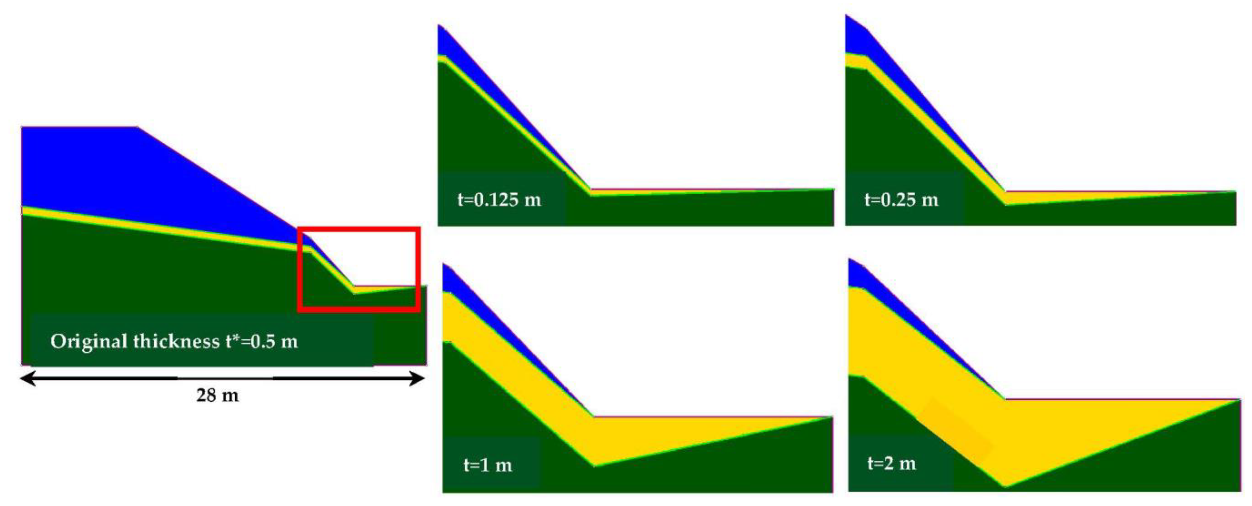
In its original configuration, the ID-1 model is characterised by a weak layer with constant thickness t* = 0.5 m. In this phase, four alternative models to the original one were realised, in which the thickness of the weak layer is one-fourth, half, double, and quadruple of t*, i.e., 0.125 m, 0.25 m, 1.0 m, and 2.0 m, respectively. They are shown in detail in Figure 11. Results of FEM analyses on the four models with a uniform mesh in the whole domain are reported in Table 8.
It should be pointed out that it was not possible to use the same total number of elements and nodes for each model, since those numbers vary depending on the internal geometry of layers, despite the constant size of the whole domain. However, the range number of elements was kept constantly between 2500 and 9000 for each analysis.
As expected, the results show how the critical SRF increases as the thickness of the weak layer decreases. In fact, when the weak-layer thickness is relatively small with respect to the model size, the rest of the domain contributes to increase the slope stability, because materials with better mechanical parameters characterise it. On the other hand, it seems that once the weak layer has reached a certain thickness size, even if it is increased, it tends not to affect the stability longer: in fact, the results for thicknesses of 1.0 m and 2.0 m are very similar to each other.
3.3.2. Lemeglio Landslide Model (LLM)
The Lemeglio Landslide Model is characterised by the presence of a thin layer of weak material (Friction Breccia) with a mean thickness of 2 m. In this phase, the thickness of the weak layer has been increased (double thickness) and decreased (half and quarter of the original thickness), in order to investigate the effect on slope stability in terms of critical SRF.
Results of the analyses carried out using a uniform mesh over the whole domain are reported in Table 9. It is possible to notice a different trend with respect to the previous ID-1 model: in fact, the different thicknesses of the weak layer do not determine significant variations in the value of the critical SRF, which is in the range 0.68–0.75. Instead, it was observed that by varying the thickness of the weak layer, significant variations in the values of the maximum shear strains occur. Results in term of maximum shear strain are reported in Table 9, as well. As it can be observed, neglecting a single anomalous case of 5499 elements (Table 9), the results seem to show the following trend: as the thickness of the weak layer decreases, the maximum shear strains tend to increase.
3.4. Analysis with Variable Outcrop Shape of the Weak Layer
In this part of the study, the analyses focused on the slope toe, particularly, on the variable shape of the weak layer at the intersection with the slope surface, which is also called the “outcrop”.
3.4.1. Model ID-1
The original outcrop of the weak layer of ID-1 model was concentrated along the horizontal plane at the slope foot [2] (Figure 12a). The outcrop elevation, which represents the intersection with the slope surface, was, therefore, raised to a vertical height of 0.3 m (Figure 12b).
By keeping the thickness of the weak layer equal to 0.5 m and varying only the outcrop shape, a uniform mesh was created over the entire slope domain, obtaining the results reported in Table 10. It can be noticed how in the original model ID-1a, the critical SRF varied in the range 1.02–0.85; instead, with a modified outcrop in ID-1b, stability conditions are different, and the critical SRF assumes lower values, varying between 0.81 and 0.71. For this model, if the weak layer outcrops along the slope surface, the overall stability is lower than in the original configuration.
As far as the maximum shear strains are concerned (not reported here), there is a significant fluctuation in their values: in fact, they change from an average value of 0.047 in the original model (ID-1a) to an average value of 0.013 for the modified outcrop (ID-1b).
3.4.2. Model ID-2
Due to its simple geometry, model ID-2 appears very useful to analyse the different outcrop shapes of the weak layer. In its original configuration, the weak layer did not intersect the slope surface, but ended exactly at the slope base, as shown in Figure 13a.
Further, three different models with different foot outcrop shapes were produced; Figure 13 shows the details of the set of models used. Specifically, in model ID-2b, the weak layer outcrops only partially (Figure 13b); in model ID-2c, the weak layer fully outcrops at the slope foot (Figure 13c); and in model ID-2d, the weak layer continues in depth, not intersecting the slope surface.
The results of the analysis carried out with a uniform mesh on the whole domain are reported in Table 11. They show a trend very similar to that found in the model ID-1. It could be noticed that in the original configuration (ID-2a), the critical SRF varied between 0.55 and 0.47, as the weak layer intersects the slope. Instead, in the model ID-2b, the critical SRF varies between 0.48 and 0.40, and in the model ID-2c, i.e., when the outcrop is total, the critical SRF drastically decreases to 0.20 and oscillates, with values very close to zero. Vice versa, for the condition reported in Figure 13d, the results show a clear improvement in the stability conditions: in fact, the values of the critical SRF are not only higher than those of the original configuration, but tend to assume almost constant values, varying within a narrow range, between 0.86 and 0.84. However, it should be pointed out that in each of these configurations, the results are below the unit value of the critical SRF.
As far as the maximum shear strains are concerned, there are no significant variations in the average values for each configuration: from 0.039 for ID-2b (partial outcrop), to 0.142 for ID-2c (total outcrop) and 0.013 for ID-2d (not any outcrop).
3.4.3. Lemeglio Landslide Model (LLM)
The effect of the outcrop shape of the weak layer was also analysed on the terminal portion of the Lemeglio landslide, which faces the sea. In the original configuration, LLM-a, shown in Figure 14a, the outcrop close to the sea level is very small (8 cm), and the thickness in the upstream portion is 2 m.
The aim of the investigation was analysing the effect of the shape of the end section of the weak layer (or Friction Breccia—FB) on the global slope stability, by keeping constant its thickness equal to 2 m. Specifically, the following three configurations were created and analysed: (1) outcrop of larger dimensions than the original one (LLMb—Figure 14b); (2) shallow weak layer not intersecting the slope surface (LLMc—Figure 14c); (3) deep weak layer not intersecting the slope surface (LLMd—Figure 14d).
In model LLMb, the weak friction layer intersects the slope surface, as in the original model (LLMa), but, unlike the original model, the outcrop is larger in size: the weak layer emerges on the slope surface reaching approximately 5 m in height.
The model LLMc (Figure 14c) is characterised by the fact that the weak layer does not intersect the slope surface, but it continues below it to a depth of approximately 8–10 m. In model LLMd (Figure 14d), the weak friction material does not intersect the slope surface, but, unlike the previous model, continues to a greater depth, varying from 18 to 58 m. In all these models, the uniform mesh has been adopted. Results are analysed in terms of critical SRF and are reported in Table 12.
It can be observed how a greater outcrop of friction material does not lead to substantial variations in terms of slope stability with respect to the original configuration: in any case, the critical SRF oscillates around values close to 0.7. In fact, as regards LLMb, the critical SRF value varies between 0.69 and 0.73.
This is also the case of LLMc, where, apart from the slightly higher value of 1622 elements, the critical SRF value varies between 0.68 and 0.73. Instead, in LLMd, the critical SRF values are above 2.5, which means that the slope is stable and in favourable condition.
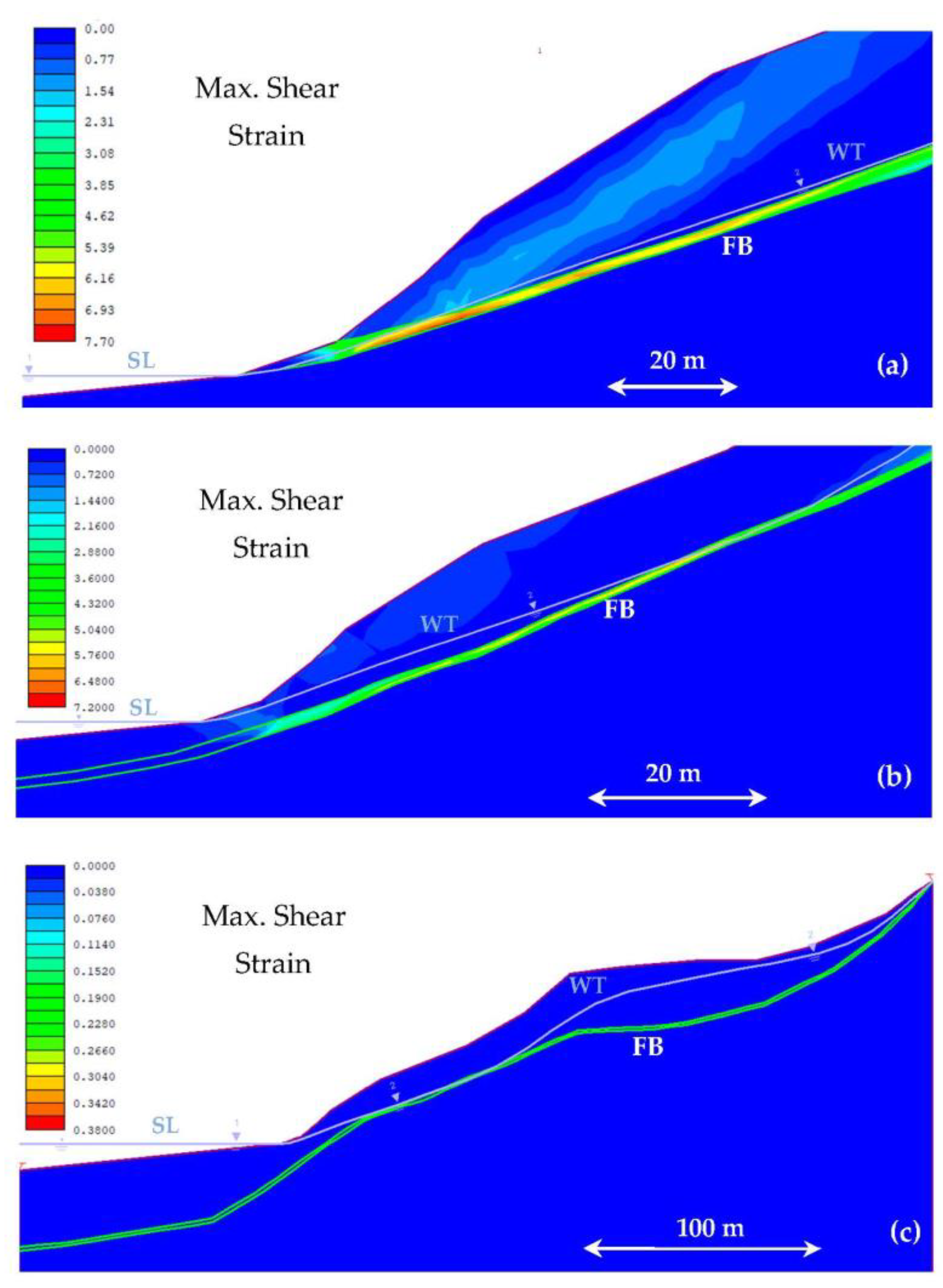
As far as the maximum shear strains are concerned, they tend to remain rather constant in the LLMb and LLMc, with values varying in both cases between 7.15 and 8.25 (Figure 15a,b, respectively). Instead, a clear reduction of maximum shear strain is observed in LLMd, where it assumes a constant value of 0.38 (Figure 15c).
3.5. Combination of Analyses: Thickness Variation with Densified Mesh
The combination of two previous situations has been analysed on model ID-1, in order to evaluate the influence of the densified mesh within the weak layer and variation of its thickness. By analysing model ID-1 with the original thickness, it has already been ascertained that four levels of mesh densification in the weak layer did not determine significant variations in the critical SRF with respect to the uniform mesh (Section 3.2.1). The only “jump” was between the results with a uniform mesh and the first level of densification, with variations of 10% in the critical SRF.
Further, three models with varying thicknesses (t = 1.0 m, t = 0.25 m, and t = 0.125 m) gradually densifying the mesh within the weak layer only were tested. For the model with the weak layer 1 m thick, results showed an almost constant trend of the critical SRF, which, despite the 3 levels of densification, varied between 0.73 and 0.79. As in the case with the original thickness (t* = 0.5 m), even with t = 1 m, there is only a slight oscillation of 10% in the values of the critical SRF by comparing results with a uniform mesh and the first level of densification. A similar trend has been observed also for the model with t = 0.25 m, where the critical SRF varies between 0.93 and 1.02. An oscillation of 10% between the uniform mesh and first level of densification has been observed even in this case.
Finally, even the model with t = 0.125 m presents a critical SRF that varies modestly by 0.09, comparing the uniform mesh and the first densification, and then settles down in the subsequent levels of densification, varying by only 0.03. The results obtained are, therefore, globally in line with those already found from the analyses related to the gradual densification of the mesh in the weak layer only.
3.6. Combination of Analyses: Mesh Densification by Element Type
A further analysis regarded the combination of two investigations on model ID-1: mesh densification in the weak layer only and variation of the type of mesh elements. The analyses were carried out by densifying the mesh only once for the four types of elements, since, after the first densification level, a stable trend was attained, as highlighted in previous analyses.
The results reported in Table 13 show the critical SRF values obtained for the mesh with 6-nodes triangles, 3-nodes triangles, 4-nodes quadrilaterals, and 8-nodes quadrilaterals. Once again, the meshes with intermediate nodes prove to be the most conservative, attaining critical SRF values that are concentrated in narrow ranges, with differences in the order of 0.04 for the 6-nodes triangular mesh and of 0.08 for the 8-nodes quadrilateral mesh. Vice versa, the results for meshes without intermediate nodes present many more variations, ranging from stable to potentially unstable conditions, as in the case of the 3-nodes triangle mesh, whose critical SRF values oscillate between 1.12 and 0.47.
4. Discussion
The main results of the described numerical analyses can be summarised as follows, considering different items.
4.1. Mesh Type
The preliminary analysis carried out with a uniform mesh over all the slope domain, by varying the type of elements as triangles or quadrilaterals, with intermediate nodes or without, allowed highlighting how the critical SRF trend is very heterogeneous.
In particular, for meshes without intermediate nodes, both triangles and quadrilaterals, the critical SRF values are not only higher than one (safety state), but they appear very variable within wide intervals, depending on the number of elements. Vice versa, for the meshes with intermediate nodes, the trend of critical SRF values for both triangular and quadrilateral geometries falls within a less wide interval, and, therefore, the critical SRF is much more constant.
Moreover, meshes with intermediate nodes attain critical SRF values that are almost totally below one (safety threshold) and are, therefore, more precautionary than those obtained with meshes without intermediate nodes.
It was then necessary to define which of the two types of meshes with intermediate nodes would be the most appropriate for the further analysis. Numerical tests allowed concluding that, for slope stability analyses with thin weak layers, the 6-nodes triangular mesh was more reliable than the 8-nodes quadrilateral mesh for two reasons at least: results appear consistent and precautionary, and the automatic mesh generation process provides much less distorted meshes.
The same conclusions, in terms of the reliability of the results, are also confirmed by the analysis carried out combining one level of mesh densification in the weak layer and by varying the type of elements. A high variability of the critical SRF values given by meshes without intermediate nodes was still observed, even when the mesh was densified. Instead, meshes with intermediate nodes provide more precautionary and stable results.
4.2. Number of Elements and Nodes in the Mesh
The analyses carried out using the uniform mesh in the whole slope domain showed a slight difference in the results for ID-1 and ID-2 models compared to the Lemeglio Landslide Model (LLM).
In fact, in models ID-1 and ID-2, the increase in the number of mesh elements and nodes determined a decreasing trend of the critical SRF, which corresponded to results that are more cautious.
As regards LLM, the critical SRF trend, by increasing the number of nodes and elements, presented a certain oscillation, which, however, given the narrow range of variation, can be considered negligible.
It can, therefore, be affirmed that, despite the greater computational time, increasing the number of elements and nodes of the mesh allows obtaining critical SRF values that are generally more cautious with respect to those obtained with a lower number of elements and nodes. This conclusion is even more valid for models with ideal geometries and reduced dimensions, where this trend is more evident with respect to real models.
4.3. Influence of the Densified Mesh in the Weak Layer
The analyses carried out by densifying the mesh within the weak layer only highlighted almost the same trend for all the models.
Results show how, even increasing the number of nodes and elements in the weak layer only, the trend of the critical SRF remains almost constant, oscillating only in the transition between the uniform mesh and the first level of densification.
4.4. Influence of the Variability of the Thickness of the Weak Layer
The influence of the thickness of the weak layer on the slope stability produced heterogeneous results that deserve further investigation.
In the ID-1 model, the variation of the weak-layer thickness produced significant fluctuations in the critical SRF, leading to the conclusion that the thinner the weak layer, the better the slope stability conditions would be.
On the other hand, in the real model of the Lemeglio landslide, despite doubling or halving the original 2 m thickness of the weak layer composed by the Friction Breccia, no oscillations in the critical SRF were found: instead, it remained almost constant.
This variable influence of the weak layer on the stability conditions, whether ideal or real models, seems to be determined by a particular effect, which seems to be a “scale effect”.
Taking into account the thickness of the weak layer (t) and the total height of each model (H), we can, therefore, define for each model a particular scaling factor λ:
ID-1 model λ = t/H = 0.5 m/15 m = 0.03
ID-2 model λ = t/H = 0.5 m/5 m = 0.1
LLM model λ = t/H = 2 m/300 m ≅ 0.007
It is evident how the scaling factor λ changes one order of magnitude passing from model ID-2, to model ID-1, to the LLM. It seems that for models with a larger scale factor λ, the influence of the variable thickness of the weak layer is more important, since the thickness itself represents a more relevant fraction of the slope and, therefore, characterises its behaviour more strongly. Vice versa, for the LLM, where the factor λ is one or two orders of magnitude smaller than the previous ones, the influence of the thickness and, therefore, of its variation is clearly lower.
Based on these considerations, the following practical conclusion can be formulated: in the case of investigations on a real landslide, characterised by considerable size and by the presence of a thin weak layer, if the λ coefficient is in the order of 10−3, the influence of the weak-layer thickness and of its spatial variation is relatively negligible on the global stability. This would be useful when, for example, it could be difficult characterising the stratigraphic continuity of the weak layer (or the presence of a friction material) at great depths or in areas that are particularly difficult to reach for in situ investigations.
4.5. Influence of the Weak-Layer Outcrop Shape
The stability analyses conducted on the variation of the outcrop shape of the weak material on the slope, both on real and ideal models, have provided clear evidence on unstable conditions. If the weak layer intersects the slope and emerges on the surface, unstable conditions are much more likely to occur with respect to the configuration in which the weak layer continues in depth, without emerging on the surface.
From the analyses carried out, it is evident that the portion of the slope that has proved to be the most sensitive to stratigraphic variations is the slope foot.
5. Conclusions
In conclusion, when conducting numerical analyses using a 2D finite element method, a number of numerical and technical practical aspects can be summarised in order to obtain precautionary results. These aspects are listed below.
- Numerical aspects:
- The 6-nodes triangle mesh is the most reliable, since it provides more consistent results than other meshes, and because it is able to produce much less distorted meshes.
- The meshes characterised by a higher number of elements and nodes allow obtaining values of the critical SRF that are more cautious than those obtained with a low number of elements and nodes, despite a greater computational time, which, nevertheless, remains acceptable.
- The first level of densification of the mesh, in the weak layer only, allows for results that are already acceptable, since the subsequent levels of densification have shown a general constancy and immutability of the critical SRF values.
- Technical and practical aspects:
- Given the variability of the results, depending on the geometry of the outcrop of the weak layer on the slope surface, it is necessary to preliminarily define in detail the geometry of the weak layer at the foot for an appropriate modelling and avoiding the risk of obtaining false results.
- It is important to define the geometry of the weak layer in advance, for example, by means of surveys and/or geophysical prospections, both in terms of the “continuity” of the weak layer and in terms of the “relative” thickness, i.e., referring to the actual dimensions of the slope under analysis.
- The λ coefficient has been defined as the ratio between the thickness of the weak layer (t) and the total height of each model (H). In the case of investigations on a very big landslide, if the λ coefficient is in the order of 10−3, the thickness and the spatial variation of the weak layer could be considered relatively negligible on the global stability, although its presence is to be taken into due consideration.
Funding
This research received no external funding.
Data Availability Statement
Data are available on request.
Acknowledgments
The author thanks Alberto Fazzi for his valuable support in carrying out the numerical analyses. The author is also grateful to the editors and reviewers, who made it possible to improve the paper.
Conflicts of Interest
The author declares no conflict of interest.
References
- Cheng, Y.M. Location of critical failure surface and some further studies on slope stability analysis. Comput. Geotech. 2003, 30, 255–267. [Google Scholar] [CrossRef]
- Cheng, Y.M.; Lansivaara, T.; Wei, W.B. Two-dimensional slope stability analysis by limit equilibrium and strength reduction methods. Comput. Geotech. 2007, 34, 137–150. [Google Scholar] [CrossRef]
- Huang, M.; Wang, H.; Sheng, D.; Liu, Y. Rotational–translational mechanism for the upper bound stability analysis of slopes with weak interlayer. Comput. Geotech. 2013, 53, 133–141. [Google Scholar] [CrossRef]
- Lim, K.; Li, A.J.; Schmid, A.; Lyamin, A.V. Slope-Stability Assessments Using Finite-Element Limit-Analysis Methods. Int. J. Geomech. 2017, 17, 06016017. [Google Scholar] [CrossRef]
- Elkamhawy, E.; Wang, H.; Zhou, B.; Yang, Z. Failure mechanism of a slope with a thin soft band triggered by intensive rainfall. Environ. Earth Sci. 2018, 77, 340. [Google Scholar] [CrossRef]
- Chen, X.; Zhang, L.; Chen, L.; Li, X.; Liu, D. Slope stability analysis based on the Coupled Eulerian-Lagrangian finite element method. Bull. Eng. Geol. Environ. 2019, 78, 4451–4463. [Google Scholar] [CrossRef]
- Zhang, W.; Wang, D. Stability analysis of cut slope with shear band propagation along a weak layer. Comput. Geotech. 2020, 125, 103676. [Google Scholar] [CrossRef]
- Sun, L.; Grasselli, G.; Liu, Q.; Thang, X.; Abdelaziz, A. The role of discontinuities in rock slope stability: Insights from a combined finite-discrete element simulation. Comput. Geotech. 2022, 147, 104788. [Google Scholar] [CrossRef]
- Yi, S.; Chen, J.; Pan, J.; Huang, J.; Qiu, Y. Risk assessment of a layered slope considering spatial variabilities of interlayer and intralayer. Comput. Geotech. 2023, 156, 105236. [Google Scholar] [CrossRef]
- Eberhardt, E.; Steadb, D.; Cogganc, J.S. Numerical analysis of initiation and progressive failure in natural rock slopes—The 1991 Randa rockslide. Int. J. Rock Mech. Min. Sci. 2004, 41, 69–87. [Google Scholar] [CrossRef]
- Cheng, Y.M. Global optimization analysis of slope stability by simulated annealing with dynamic bounds and Dirac function. Eng. Optim. 2007, 39, 17–32. [Google Scholar]
- Wei, W.B.; Cheng, Y.M.; Li, L. Three-dimensional slope failure analysis by the strength reduction and limit equilibrium methods. Comput. Geotech. 2009, 36, 70–80. [Google Scholar] [CrossRef]
- Cevasco, A.; Termini, F.; Valentino, R.; Meisina, C.; Bonì, R.; Bordoni, M.; Chella, G.P.; De Vita, P. Residual mechanisms and kinematics of the relict Lemeglio coastal landslide (Liguria, northwestern Italy). Geomorphology 2018, 320, 64–81. [Google Scholar] [CrossRef]
Figure 1.
Ideal model ID-1, modified from [2]. TL = Top Layer (blue); WL = Weak Layer (yellow); BL = Bottom Layer (dark green).
Figure 1.
Ideal model ID-1, modified from [2]. TL = Top Layer (blue); WL = Weak Layer (yellow); BL = Bottom Layer (dark green).

Figure 2.
Ideal model ID-2, modified from [12]. TL = Top Layer (blue); WL = Weak Layer (yellow); BL = Bottom Layer (dark green).
Figure 2.
Ideal model ID-2, modified from [12]. TL = Top Layer (blue); WL = Weak Layer (yellow); BL = Bottom Layer (dark green).

Figure 3.
Lemeglio Landslide Model (LLM), modified from [13]. LD = Landslide Deposit (light green); FB = Friction Breccia (green); FBS = Forcella Bended Shale (beige); 1 = Sea Level (grey line); 2 = Water Table (grey line).
Figure 3.
Lemeglio Landslide Model (LLM), modified from [13]. LD = Landslide Deposit (light green); FB = Friction Breccia (green); FBS = Forcella Bended Shale (beige); 1 = Sea Level (grey line); 2 = Water Table (grey line).

Figure 4.
Details of ID-1 model. Different meshes of the weak layer based on different total number of elements (N): (a) N = 1500; (b) N = 4500; (c) N = 7500; (d) N = 9000 (blue = Top layer; yellow = Weak layer; dark green = Bottom layer).
Figure 4.
Details of ID-1 model. Different meshes of the weak layer based on different total number of elements (N): (a) N = 1500; (b) N = 4500; (c) N = 7500; (d) N = 9000 (blue = Top layer; yellow = Weak layer; dark green = Bottom layer).

Figure 5.
Details of model ID-1. Different levels of mesh densification in the weak layer: (a) Uniform mesh; (b) Mesh intensified 2 times (blue = Top layer; yellow = Weak layer; dark green = Bottom layer).
Figure 5.
Details of model ID-1. Different levels of mesh densification in the weak layer: (a) Uniform mesh; (b) Mesh intensified 2 times (blue = Top layer; yellow = Weak layer; dark green = Bottom layer).

Figure 6.
Model ID-1 with 6-nodes uniform triangular mesh: FEM results in terms of maximum shear strain (RS2).
Figure 6.
Model ID-1 with 6-nodes uniform triangular mesh: FEM results in terms of maximum shear strain (RS2).

Figure 7.
Model ID-2 with 6-nodes uniform triangular mesh: FEM results in terms of maximum shear strain (RS2) (Critical SRF = 0.55).
Figure 7.
Model ID-2 with 6-nodes uniform triangular mesh: FEM results in terms of maximum shear strain (RS2) (Critical SRF = 0.55).

Figure 8.
LLM with 6-nodes uniform triangular mesh: FEM results in terms of maximum shear strain (RS2) (Critical SRF = 0.7).
Figure 8.
LLM with 6-nodes uniform triangular mesh: FEM results in terms of maximum shear strain (RS2) (Critical SRF = 0.7).

Figure 9.
ID-1 model: maximum shear strain with (a) uniform mesh and (b) after the 2nd level of mesh densification in the weak layer only.
Figure 9.
ID-1 model: maximum shear strain with (a) uniform mesh and (b) after the 2nd level of mesh densification in the weak layer only.

Figure 10.
LLM: detail of the weak layer (red window) with (a) uniform mesh and (b) after the 3rd level of mash densification. SL = Sea Level; WT = Water Table; FB = Friction Breccia. Light green = Landslide Deposit; Yellow = Friction Breccia; Pink = Forcella Bended Shale.
Figure 10.
LLM: detail of the weak layer (red window) with (a) uniform mesh and (b) after the 3rd level of mash densification. SL = Sea Level; WT = Water Table; FB = Friction Breccia. Light green = Landslide Deposit; Yellow = Friction Breccia; Pink = Forcella Bended Shale.

Figure 11.
Model ID-1. Details of the four models with different thickness of the weak layer (blue = Top layer; yellow = Weak layer; dark green = Bottom layer).
Figure 11.
Model ID-1. Details of the four models with different thickness of the weak layer (blue = Top layer; yellow = Weak layer; dark green = Bottom layer).

Figure 12.
Model ID-1. Details of the variable outcrop of the weak layer (blue = Top layer; yellow = Weak layer; dark green = Bottom layer).
Figure 12.
Model ID-1. Details of the variable outcrop of the weak layer (blue = Top layer; yellow = Weak layer; dark green = Bottom layer).

Figure 13.
Model ID-2. Details representing different geometries of the weak-layer toe: (a) Original outcrop; (b) Partial outcrop; (c) Total outcrop; (d) Absent outcrop (blue = Top layer; yellow = Weak layer; dark green = Bottom layer).
Figure 13.
Model ID-2. Details representing different geometries of the weak-layer toe: (a) Original outcrop; (b) Partial outcrop; (c) Total outcrop; (d) Absent outcrop (blue = Top layer; yellow = Weak layer; dark green = Bottom layer).

Figure 14.
Lemeglio Landslide Model (LLM). Details representing different geometries of the weak-layer outcrop made of Friction Breccia (FB): (a) Original outcrop (LLMa); (b) outcrop with larger dimensions than the original (LLMb); (c) shallow weak layer not intersecting the slope surface (LLMc); (d) deep weak layer not intersecting the slope surface (LLMd). SL = Sea Level; WT = Water Table. Light green = Landslide Deposit; Yellow/Green = Friction Breccia; Pink = Forcella Bended Shale.

Figure 15.
Lemeglio Landslide Model (LLM). Details representing the maximum shear strain for different geometries of the weak-layer toe: (a) outcrop with larger dimensions than the original (LLMb); (b) shallow weak layer that does not intersect the slope surface (LLMc); (c) deep weak layer that does not intersect the slope surface (LLMd). SL = Sea Level; WT = Water Table; FB = Friction Breccia.


Table 1.
Input parameters of the numerical models.
| Model | Soil/Rock Layer | Effective Cohesion (kPa) | Friction Angle (°) | Unit Weight (kN/m3) | Elastic Modulus (MPa) | Poisson’s Ratio (-) |
|---|---|---|---|---|---|---|
| ID-1 | Top layer (TL) | 20 | 35 | 19 | 14 | 0.3 |
| Weak layer (WL) | 0 | 25 | 19 | 14 | 0.3 | |
| Bottom layer (BL) | 10 | 35 | 19 | 14 | 0.3 | |
| ID-2 | Top layer (TL) | 20 | 35 | 19 | 14 | 0.3 |
| Weak layer (WL) | 0 | 25 | 19 | 14 | 0.3 | |
| Bottom layer (BL) | 10 | 35 | 19 | 14 | 0.3 | |
| LLM | Landslide Deposit (LD) | 0 | 40 | 20 | 200 | 0.3 |
| Friction Breccia (FB) | 0 | 26 | 18 | 40 | 0.3 | |
| Forcella Banded Shale (FBS) | 2050 | 35 | 25 | 1643 | 0.3 |
Table 2.
Model ID-1 with uniform mesh.
| 3-Nodes Triangular | 6-Nodes Triangular | 4-Nodes Quadrilateral | 8-Nodes Quadrilateral | ||||||||
|---|---|---|---|---|---|---|---|---|---|---|---|
| El. | Nodes | C. SRF | El. | Nodes | C. SRF | El. | Nodes | C. SRF | El. | Nodes | C. SRF |
| 1857 | 987 | 1.65 | 1857 | 3830 | 1.02 | 1933 | 2020 | 1.13 | 1933 | 5972 | 0.85 |
| 2856 | 1511 | 1.40 | 2856 | 5877 | 1.00 | 3157 | 3276 | 1.18 | 3157 | 9708 | 0.84 |
| 3427 | 1815 | 1.17 | 3427 | 7056 | 0.94 | 4080 | 4219 | 1.12 | 4080 | 12,517 | 0.82 |
| 3868 | 2051 | 1.26 | 3868 | 7696 | 0.98 | 4921 | 5077 | 1.12 | 4921 | 15,074 | 0.83 |
| 8116 | 4188 | 1.15 | 8116 | 26,491 | 0.86 | 5605 | 5777 | 1.06 | 5605 | 17,158 | 0.82 |
| 9006 | 4646 | 1.16 | 9006 | 18,297 | 0.85 | 10,101 | 10,397 | 1.03 | 10,101 | 30,724 | 0.80 |
El.: No. of elements in the mesh; Nodes: No. of nodes in the mesh; C. SRF: critical SRF.
Table 3.
Results obtained by Cheng et al. (2007) for the same ID-1 model (domain length 28 m, 4-nodes quadrilateral mesh).
Table 3.
Results obtained by Cheng et al. (2007) for the same ID-1 model (domain length 28 m, 4-nodes quadrilateral mesh).
| Numerical Code | Critical SRF–SRM1 | Critical SRF–SRM2 |
|---|---|---|
| Flac 3D | 1.64 | 1.61 |
| Phase | 0.87 | 1.37 |
| Plaxis | 0.86 | 0.97 |
Table 4.
Model ID-2 and Lemeglio Landslide Model (LLM) with uniform 6-nodes triangular mesh.
| Model ID-2 | LLM | ||||
|---|---|---|---|---|---|
| No. Elements | No. Nodes | Critical SRF | No. Elements | No. Nodes | Critical SRF |
| 1387 | 2882 | 0.55 | 1714 | 3529 | 0.74 |
| 2972 | 6099 | 0.52 | 3756 | 7651 | 0.73 |
| 5915 | 12,054 | 0.50 | 5757 | 11,680 | 0.71 |
| 9263 | 18,749 | 0.47 | 9823 | 19,856 | 0.70 |
Table 5.
Model ID-1 with increase of mesh density in the weak layer (6-nodes triangular mesh).
| Uniform Mesh | 1st Densification | 2nd Densification | 3rd Densification | 4th Densification | ||||||||||
|---|---|---|---|---|---|---|---|---|---|---|---|---|---|---|
| El. | Nodes | C. SRF | El. | Nodes | C. SRF | El. | Nodes | C. SRF | El. | Nodes | C. SRF | El. | Nodes | C. SRF |
| 1857 | 3830 | 1.02 | 2071 | 4258 | 0.85 | 2713 | 5542 | 0.83 | 4639 | 9394 | 0.82 | 10,417 | 20,950 | 0.80 |
| 2856 | 5877 | 1.00 | 3186 | 6537 | 0.83 | 4176 | 8517 | 0.80 | 7146 | 14,457 | 0.77 | 16,056 | 32,207 | 0.79 |
| 3427 | 7056 | 0.94 | 3829 | 7860 | 0.83 | 5035 | 10,272 | 0.80 | 8653 | 17,508 | 0.80 | - | - | - |
| 3868 | 7696 | 0.98 | 4356 | 8945 | 0.83 | 5820 | 11,873 | 0.80 | - | - | - | - | - | - |
| 8116 | 26,491 | 0.86 | 8980 | 18,219 | 0.80 | 11,572 | 23,403 | 0.78 | - | - | - | - | - | - |
| 9006 | 18,297 | 0.85 | 9966 | 20,217 | 0.81 | 12,846 | 25,977 | 0.77 | - | - | - | - | - | - |
El.: No. of elements in the mesh; Nodes: No. of nodes in the mesh; C. SRF: critical SRF.
Table 6.
Model ID-2 with increase of mesh density in the weak layer (6-nodes triangular mesh).
| Uniform Mesh | 1st Densification | 2nd Densification | 3rd Densification | ||||||||
|---|---|---|---|---|---|---|---|---|---|---|---|
| El. | Nodes | C. SRF | El. | Nodes | C. SRF | El. | Nodes | C. SRF | El. | Nodes | C. SRF |
| 1387 | 2882 | 0.55 | 1739 | 3586 | 0.55 | 2795 | 5698 | 0.54 | 5963 | 12,034 | 0.48 |
| 2972 | 6099 | 0.52 | 3664 | 7483 | 0.50 | 5740 | 11,635 | 0.50 | 11,698 | 24,091 | 0.45 |
| 5915 | 12,054 | 0.50 | 5193 | 10,574 | 0.48 | - | - | - | . | - | - |
| 9263 | 18,749 | 0.47 | 9154 | 19,559 | 0.49 | - | - | - | - | - | - |
El.: No. of elements in the mesh; Nodes: No. of nodes in the mesh; C. SRF: critical SRF.
Table 7.
LLM with increase of mesh density in the weak layer (6-nodes triangular mesh).
| Uniform Mesh | 1st Densification | 2nd Densification | 3rd Densification | 4th Densification | ||||||||||
|---|---|---|---|---|---|---|---|---|---|---|---|---|---|---|
| El. | Nodes | C. SRF (*MSS) | El. | Nodes | C. SRF (*MSS) | El. | Nodes | C. SRF (*MSS) | El. | Nodes | C. SRF (*MSS) | El. | Nodes | C. SRF (*MSS) |
| 1714 | 3529 | 0.74 | 1976 | 4053 | 0.73 | 2762 | 5625 | 0.72 | 5120 | 10,341 | 0.73 | 12,194 | 24,489 | 0.74 |
| 3756 | 7651 | 0.73 *8.31 | 4042 | 8223 | 0.72 *9.86 | 4900 | 9939 | 0.72 *10.26 | 7474 | 15,087 | 0.72 *10.86 | 15,196 | 30,351 | 0.71 *11.02 |
El.: No. of elements in the mesh; Nodes: No. of nodes in the mesh; C. SRF: critical SRF; MSS: Maximum Shear Strain.
Table 8.
Model ID-1 with different thickness (t) of the weak layer (6-nodes triangular uniform mesh).
Table 8.
Model ID-1 with different thickness (t) of the weak layer (6-nodes triangular uniform mesh).
| t* = 0.5 m | t = 0.125 m (t* × 0.25) | t = 0.25 m (t* × 0.5) | t = 1.0 m (t* × 2) | t = 2.0 m (t* × 4) | ||||||||||
|---|---|---|---|---|---|---|---|---|---|---|---|---|---|---|
| El. | Nodes | C. SRF | El. | Nodes | C. SRF | El. | Nodes | C. SRF | El. | Nodes | C. SRF | El. | Nodes | C. SRF |
| 1857 | 3830 | 1.02 | 3060 | 6227 | 1.19 | 2881 | 5758 | 1.12 | 2858 | 5881 | 0.86 | 2860 | 5885 | 0.87 |
| 2856 | 5877 | 1.00 | 4590 | 9313 | 1.17 | 4626 | 9417 | 1.09 | 3447 | 7096 | 0.85 | 4443 | 9096 | 0.77 |
| 3427 | 7056 | 0.94 | 5956 | 12,069 | 1.19 | 6102 | 12,407 | 1.05 | 5552 | 11,337 | 0.79 | 6241 | 12,730 | 0.79 |
| 3868 | 7696 | 0.98 | 7577 | 15,334 | 1.14 | 7075 | 14,384 | 1.05 | 6433 | 13,124 | 0.79 | 7641 | 15,188 | 0.79 |
| 8116 | 26,491 | 0.86 | 9184 | 18,571 | 1.13 | 8086 | 16,431 | 1.04 | 9008 | 18,301 | 0.78 | - | - | - |
| 9006 | 18,297 | 0.85 | - | - | - | 9012 | 18,309 | 1.04 | - | - | - | - | - | - |
El.: No. of elements in the mesh; Nodes: No. of nodes in the mesh; C. SRF: critical SRF.
Table 9.
LLM with different thicknesses (t) of the weak layer (6-nodes triangular uniform mesh).
| t* = 2 m (Table 4) | t = 4 m (t* × 2) | t = 1 m (t* × 0.5) | t = 0.5 m (t* × 0.25) | |||||||||||
|---|---|---|---|---|---|---|---|---|---|---|---|---|---|---|
| El. | Nodes | C. SRF | El. | Nodes | C. SRF | MSS | El. | Nodes | C. SRF | MSS | El. | Nodes | C. SRF | MSS |
| 1714 | 3529 | 0.74 | 1689 | 3480 | 0.75 | 6.02 | 1728 | 3559 | 0.73 | 12.42 | 1739 | 3604 | 0.72 | 17.06 |
| 3756 | 7651 | 0.73 | 3625 | 7390 | 0.74 | 6.31 | 3768 | 7677 | 0.72 | 12.61 | 3363 | 6910 | 0.70 | 15.39 |
| 5757 | 11,680 | 0.71 | 5499 | 11,170 | 0.70 | 3.04 | 5758 | 11,689 | 0.71 | 11.64 | 5664 | 11,563 | 0.70 | 16.19 |
| 9823 | 19,856 | 0.70 | 9462 | 19,143 | 0.69 | 7.08 | 9861 | 19,934 | 0.69 | 12.79 | 9554 | 19,399 | 0.68 | 15.93 |
El.: No. of elements in the mesh; Nodes: No. of nodes in the mesh; C. SRF: critical SRF; MSS: Maximum Shear Strain.
Table 10.
Model ID-1 with different outcrop shapes of the weak layer (6-nodes triangular mesh).
| ID-1a | ID-1b | ||||
|---|---|---|---|---|---|
| El. | Nodes | C. SRF | El. | Nodes | C. SRF |
| 1857 | 3830 | 1.02 | 2226 | 4569 | 0.81 |
| 2856 | 5877 | 1.00 | 3376 | 6917 | 0.82 |
| 3427 | 7056 | 0.94 | 3858 | 7949 | 0.78 |
| 3868 | 7696 | 0.98 | 6438 | 13,135 | 0.77 |
| 8116 | 26,491 | 0.86 | 12,911 | 26,152 | 0.71 |
| 9006 | 18,297 | 0.85 | - | - | - |
El.: No. of elements in the mesh; Nodes: No. of nodes in the mesh; C. SRF: critical SRF.
Table 11.
Model ID-2 with different outcrop shapes of the weak layer (6-nodes triangular mesh).
| ID-2a | ID-2b | ID-2c | ID-2d | ||||||||
|---|---|---|---|---|---|---|---|---|---|---|---|
| El. | Nodes | C. SRF | El. | Nodes | C. SRF | El. | Nodes | C. SRF | El. | Nodes | C. SRF |
| 1387 | 2882 | 0.55 | 1435 | 2998 | 0.48 | 1612 | 3337 | 0.20 | 1410 | 2931 | 0.86 |
| 2972 | 6099 | 0.52 | 2946 | 6051 | 0.35 | 2950 | 6057 | 0.13 | 2982 | 6119 | 0.85 |
| 5915 | 12,054 | 0.50 | 4117 | 8440 | 0.36 | 4111 | 8408 | 0.13 | 4179 | 8544 | 0.85 |
| 9263 | 18,749 | 0.47 | 5675 | 11,574 | 0.38 | 6047 | 12,320 | 0.04 | 6066 | 12,361 | 0.84 |
| - | - | - | 7498 | 15,274 | 0.40 | 7497 | 15,246 | 0.03 | 7621 | 15,492 | 0.84 |
| - | - | - | 8434 | 17,159 | 0.40 | 9173 | 18,626 | 0.03 | 8827 | 17,936 | 0.84 |
El.: No. of elements in the mesh; Nodes: No. of nodes in the mesh; C. SRF: critical SRF.
Table 12.
Lemeglio Landslide Model with different outcrop shapes of the weak layer (6-nodes triangular uniform mesh).
Table 12.
Lemeglio Landslide Model with different outcrop shapes of the weak layer (6-nodes triangular uniform mesh).
| LMMa | LMMb | LMMc | LMMd | ||||||||
|---|---|---|---|---|---|---|---|---|---|---|---|
| El. | Nodes | C. SRF | El. | Nodes | C. SRF | El. | Nodes | C. SRF | El. | Nodes | C. SRF |
| 1714 | 3529 | 0.74 | 1773 | 3650 | 0.73 | 1622 | 3347 | 0.84 | 1849 | 3804 | 2.56 |
| 3756 | 7651 | 0.73 | 3559 | 7260 | 0.72 | 3649 | 7442 | 0.73 | 3769 | 7678 | 2.54 |
| 5757 | 11,680 | 0.71 | 5396 | 10,965 | 0.71 | 5543 | 11,260 | 0.73 | 5765 | 11,702 | 2.54 |
| 9823 | 19,856 | 0.70 | 9158 | 18,533 | 0.69 | 9077 | 18,470 | 0.68 | 9852 | 19,915 | 2.53 |
El.: No. of elements in the mesh; Nodes: No. of nodes in the mesh; C. SRF: critical SRF.
Table 13.
Model ID-1 with 1st level of mesh densification in the weak layer and different mesh types.
Table 13.
Model ID-1 with 1st level of mesh densification in the weak layer and different mesh types.
| Uniform Mesh 6-Nodes Triangular | 1st Densification 6-Nodes Triangular | 1st Densification 3-Nodes Triangular | 1st Densification 4-Nodes Quadrilateral | 1st Densification 8-Nodes Quadrilateral | ||||||||||
|---|---|---|---|---|---|---|---|---|---|---|---|---|---|---|
| El. | Nodes | C. SRF | El. | Nodes | C. SRF | El. | Nodes | C. SRF | El. | Nodes | C. SRF | El. | Nodes | C. SRF |
| 1857 | 3830 | 1.02 | 2071 | 4258 | 0.85 | 2071 | 1094 | 1.12 | 2080 | 2157 | 1.23 | 2080 | 6393 | 0.85 |
| 2856 | 5877 | 1.00 | 3186 | 6537 | 0.83 | 3186 | 1676 | 1.09 | 3347 | 3461 | 1.21 | 3347 | 10,265 | 0.84 |
| 3427 | 7056 | 0.94 | 3829 | 7860 | 0.83 | 3829 | 2016 | 1.11 | 4313 | 4448 | 1.00 | 4313 | 13,208 | 0.82 |
| 3868 | 7696 | 0.98 | 4356 | 8945 | 0.83 | 4356 | 2295 | 1.16 | 5181 | 5338 | 0.98 | 5181 | 15,856 | 0.80 |
| 8116 | 26,491 | 0.86 | 8980 | 18,219 | 0.80 | 8980 | 4620 | 0.99 | 5894 | 6070 | 0.47 | 5894 | 18,033 | 0.77 |
| 9006 | 18,297 | 0.85 | 9966 | 20,217 | 0.81 | 9966 | 5126 | 0.47 | 10,502 | 10,704 | 1.03 | 10,502 | 32,068 | 0.77 |
El.: No. of elements in the mesh; Nodes: No. of nodes in the mesh; C. SRF: critical SRF.
Disclaimer/Publisher’s Note: The statements, opinions and data contained in all publications are solely those of the individual author(s) and contributor(s) and not of MDPI and/or the editor(s). MDPI and/or the editor(s) disclaim responsibility for any injury to people or property resulting from any ideas, methods, instructions or products referred to in the content. |
© 2023 by the author. Licensee MDPI, Basel, Switzerland. This article is an open access article distributed under the terms and conditions of the Creative Commons Attribution (CC BY) license (https://creativecommons.org/licenses/by/4.0/).
Share and Cite
MDPI and ACS Style
Valentino, R. FEM Modelling of Thin Weak Layers in Slope Stability Analysis. Geosciences 2023, 13, 233. https://doi.org/10.3390/geosciences13080233
AMA Style
Valentino R. FEM Modelling of Thin Weak Layers in Slope Stability Analysis. Geosciences. 2023; 13(8):233. https://doi.org/10.3390/geosciences13080233
Chicago/Turabian StyleValentino, Roberto. 2023. "FEM Modelling of Thin Weak Layers in Slope Stability Analysis" Geosciences 13, no. 8: 233. https://doi.org/10.3390/geosciences13080233
Note that from the first issue of 2016, this journal uses article numbers instead of page numbers. See further details here.