Article

Tunnelling with Full-Face Shielded Machines: A 3D Numerical Analysis of an Earth Pressure Balance (EPB) Excavation Sequence Using the Finite Element Method (FEM)

1
School of Earth and Environment, University of Leeds, Leeds LS2 9JT, UK
2
Ground Engineering and Tunnelling, Ramboll, Leeds LS1 8EQ, UK
3
School of Civil Engineering, National Technical University of Athens, 106 82 Athens, Greece
*
Author to whom correspondence should be addressed.
Geosciences 2023, 13(8), 244; https://doi.org/10.3390/geosciences13080244
Submission received: 21 February 2023 / Revised: 20 July 2023 / Accepted: 10 August 2023 / Published: 12 August 2023
(This article belongs to the Special Issue Advanced Numerical Modelling and Analysis in Geotechnical Engineering)

Abstract

:
Urban tunnelling can be highly challenging, especially in areas where limited ground settlements and environmental disturbance is required. Mechanised tunnelling is usually preferred in such ground environments, specifically Slurry or EPBM (Earth Pressure Balance Machine), depending on the ground properties. Being able to predict the anticipated tunnel behaviour at the preliminary stages of the project can be very beneficial in optimising not only the design, but also control the construction activities and completion times. In practice, the short-term excavation response and support performance focus primarily on design, since most site characterisation inputs are focused on material properties gained from short-term testing. Although the analysis of tunnelling is a three-dimensional (3D) problem, conventional approaches and design methods employed during the design and construction of underground openings are often based on the ground’s static response in two dimensions (2D). In this paper, an initial 2D model is generated in PLAXIS2D and RS2 (Rocscience) to test advanced constitutive models and compare transverse settlement profiles; subsequently, a complete 3D FEM numerical model in RS3 (Rocscience) was used to simulate an Earth Pressure Balance (EPB) excavation sequence. The 3D numerical model simulates the relevant EPB components such as face pressure, TBM shield, backfilling of the tail void (time-dependent hardening of the grout) and gradual segmental lining erections in the longitudinal direction. The presented numerical approach can be used by tunnel designers and engineers to predict the soil response in EPBM tunnelling.

1. Introduction

Automation and mechanisation have become more pertinent to construction, including tunnelling. There is a shared desire to increase efficiency using faster-integrated tunnelling methods that can ultimately save costs by reducing the construction time [1]. Underground space is currently an integral part of cities and needs to be holistically considered during urban design and planning [2,3]. Consequently, there is a drive to excavate underground. Transport and utility lines are consistently requested to keep up with the population growth, which encourages the use of the Earth Pressure Balanced (EPB) TBM (Tunnel Boring Machine). These full-face shielded TBMs are faced with the technical challenge of constructing through heterogeneous subsurface conditions, with a primary focus on limiting surface deformation in the area of influence [1]. Therefore, it is paramount to understand the geology and the necessary pressure components to be applied during tunnel excavation. This research focuses on a tunnel excavation through London Clay, a formation with important engineering implications. The understanding of geotechnical properties related to rock and soils that are commonly found in urban environments at the excavated zone is important for defining the excavation method and sequence, and consequently, the front pressure needed in order to sustain front stability [4]. Numerical modelling methods and approaches in geotechnical engineering have significantly changed tunnelling design during the past decades by simulating complex TBM features required for accuracy, especially in 3D models [5,6,7]. This approach complements the tunnel design whilst also estimating project costs and project duration [8,9,10].
Generally, most investigations involve 2D plane strain analysis due to its satisfactory results. However, this method fails to incorporate the deformation effects of the excavation process in the third dimension. There has been less research on 3D modelling to synthesise multi-directional settlement predictions whilst assessing each stage’s impact on the excavation process. It is thought that 3D modelling can encompass all relevant EPB components whilst producing a more accurate deformation analysis [5]. There has been a significant focus on replicating the actual issue in 3D as close as possible using a variety of discrete soil models representing a certain lithology more accurately. RS3 [11] is one of the most recent FEM (Finite Element Method) software that has less explored capabilities of producing EPB excavation sequences. Therefore, this forms the focus of this research. PLAXIS2D [12] which is arguably an FEM software that is more opted for, will be used initially, with complexity increasing later. Most authors, including [13] argue that PLAXIS2Dsoftware should be used as validation against the RS2 and RS3 models.
The primary aim of this paper is to validate the use of the Finite Element Method (FEM) software PLAXIS2D and [11]: RS2 and RS3 combined with several constitutive models to simulate the complete tunnel excavation process in an urban environment using an Earth Pressure Balance Machine (EPBM). The proposed framework builds in complexity from an initial 2D analysis, using PLAXIS2D as a validator, to a full 3D model in RS3 to simulate the relevant components including different constitutive models of ground behaviour. The comparison among the various models is based on the predictions of the surface settlement profiles for a sewer tunnel with an 8 m diameter excavated at a 34 m depth within London Clay.

2. Background

2.1. Tunnelling in Soft Ground

Tunnelling in soft ground in urban areas is currently performed using mechanised tunnelling or Tunnel Boring Machines (TBMs). More specifically, single-shielded TBMs are designed to deliver a fully integrated tunnel system with minimal deformation to the surrounding area while balancing the interchangeable underground forces. They are usually known to operate under poor soil conditions with a low load-bearing capacity in saturated conditions [1], with the primary aim of controlling and reducing subsidence, such as prohibiting the limit states exceeded. Slurry and Earth Pressure Balance Machines (EPBMs) are the two types of single-shielded TBMs with two main functions: a. segmental lining instalment using hydraulic jacks and b. tail void grouting to successfully overcome and tunnel through weak ground conditions [14].

2.2. EPBM Tunnelling

EPBMs are generally used in ground pressures of less than 8 bars to effectively balance the earth’s pressure against the tunnel to minimise subsidence. During tunnel advancement, the shield must continuously support the overburden stress, replicating the original stress conditions. The rotating cutter head is pressed against the excavated face with a balanced pressure operated by multiple hydraulic cylinders. The Earth Pressure Balance (EPB) system efficiency is controlled by the incoming and releasing of the pressurised material within the excavation chamber, which is regulated from the screw conveyor (Figure 1). Therefore, to prevent surface settlement, the surrounding soil and water conditions should be adequately balanced [15].
During tunnel advancement, the lining installation takes place under the protection of the shield. The tunnel ring comprises multiple interlocking segments constructed of prefabricated concrete. Once a complete ring is constructed, the backfilling grout is pressurised through the tail skin into the annular gap at the interface between the soil and lining. The latter should be a continuous process; the backfilling is performed immediately to prevent the development of any void spaces. A brief description of the face pressure, the shield, the grout pressure and the segmental lining of the stages modelled in this analysis is presented.

2.2.1. Face Pressure

The coefficient of the active earth pressure is the driver for tunnel face instability, and the shear strength properties dictate the soil movement. The active earth pressure plays a more significant role in causing failure than the C/D (cover/depth) ratio [17]. Inadequate face support pressure can lead to the active overturning of the face material into the excavation and high ground displacement rates. The chamber’s pressure should be greater than the hydrostatic pore water pressure in the surrounding material to prevent seepage flow into the tunnel. Therefore, most authors adopt a trapezoidal face pressure distribution.

2.2.2. Segmental Lining

Segmental lining is constructed from prefabricated concrete segments under the shield protection using instantaneous vacuum installers forming a jointed ring. Each ring is installed concurrently to the injection of grout in the surrounding annular gap. [18] discovered that the intensity of the pressure around the lining was influenced by the grouting pressure rather than the lining itself. Higher grouting pressures initiate higher earth pressures with the non-uniform distribution.

2.3. Modelling EPBM Tunnelling

The use of 3D modelling in tunnelling has increased in popularity as this can simulate a complete excavation process, providing expected deformation in both lateral and longitudinal directions. TBM modelling often includes simulating the TBM shield, the face pressure, the segmental lining (continuous shell) and the annular gap grouting, with some cases even modelling the grout’s time hardening behaviour. In this section, only the face pressure, the shield and the segmental lining are discussed.

2.3.1. Modelling the Face Pressure

The face pressure is modelled as non-uniform trapezoidal pressure distribution based on the assumption that there is a linear increase in the pressure with depth, which also applies to saturated conditions using the hydrostatic pressure, and it should be theoretically equal to the pressure in the chamber to maintain stability. A uniform averaged pressure distribution is usually adopted, as [19] described when modelling the Madrid Metro extension project due to the variance in the excavation chamber pressure.

2.3.2. Modelling the Annular Grout

The backfilling of the annular gap is a problematic constituent of the model. It assumes that the grout is applied as a continuous layer that is subjected to the pressurised grouting system’s effectiveness [14] changed the backfilling material’s behaviour to be time dependent, which encountered a stiffness evolution throughout the excavation process from initially applied stress with no stiffness [20] to a fully hardened grout. A time-dependent stiffness increase can then be implemented with a corresponding decrease in pressure away from the shield [5].

2.3.3. Modelling the Segmental Lining

Ref. [21] and others investigated the design methods based on the assumption that the lining acted as a linear elastic circular beam after the Saint-Venant beam theory, which was created in 1855. The joints’ effects can be considered by computing a reduced flexural stiffness but this was not possible until [5] fully numerically simulated staggered jointed lining.

2.3.4. Modelling the EPBM Shield

Most authors model the shield and cutter head elastically using continuous shell elements. The excavation chamber is usually prescribed with solid elements, including nodes to provide support pressure and simulate the TBM’s weight. The latter profoundly influences the tunnel’s uplift invert, more so at shallow depths [5].

2.4. Modelling the Ground Conditions in Geotechnical Engineering for EPBM
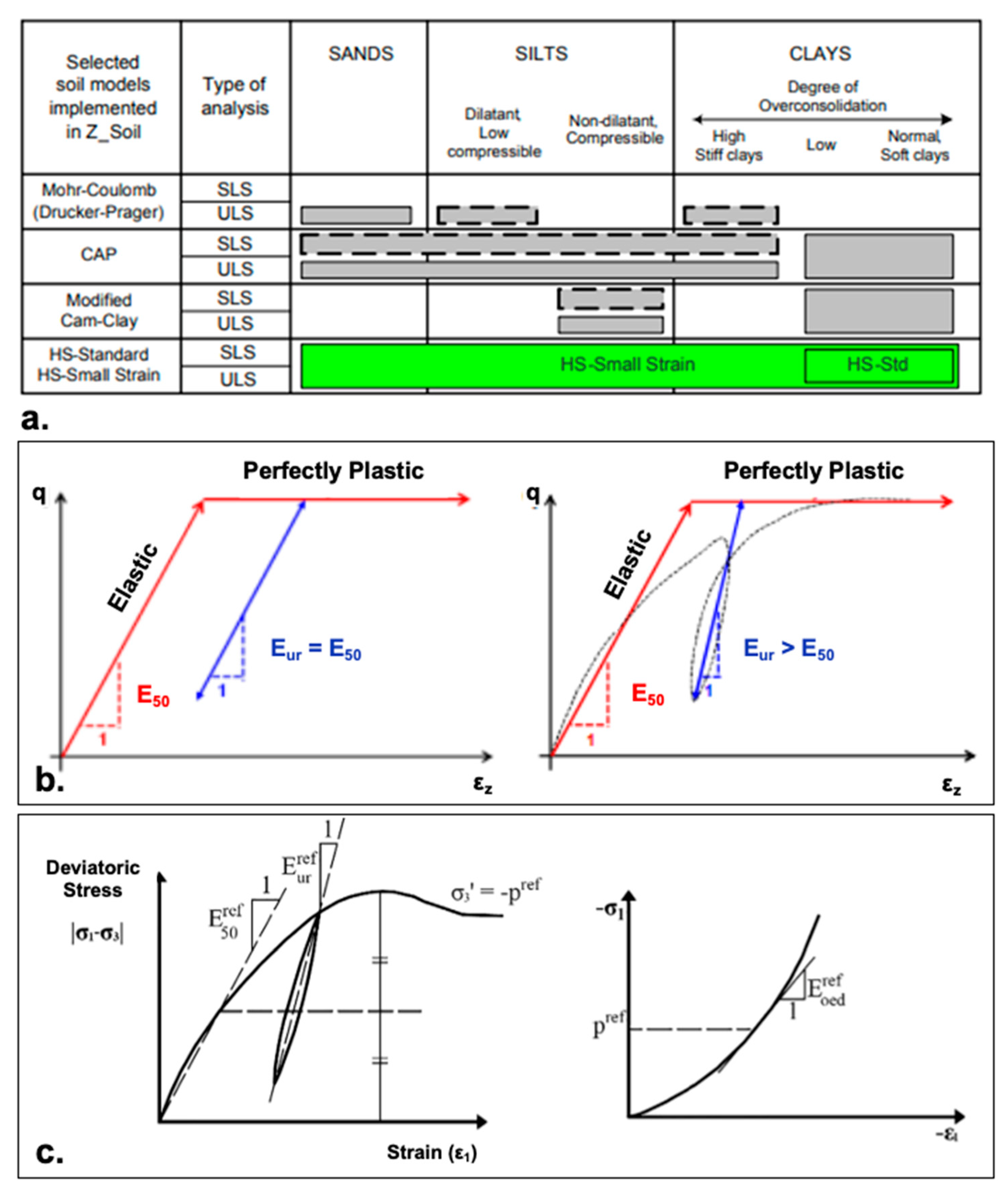
Over the past years in geotechnical engineering, a lot of work has been concentrated on simulating the geometry with sufficient complexity and accuracy, but less emphasis is usually placed on modelling ground behaviour using suitable constitutive models.

2.4.1. Mohr–Coulomb

A simple ground can be described by a linearly elastic–perfectly plastic model based on the Mohr–Coulomb (M-C) criterion. However, this model fails to accurately replicate significant soil deformation characteristics in cohesive material such as London Clay. According to [22], the choice of a constitutive model is predominantly related to the type of analysis needed to be undertaken for the Ultimate Limit State (ULS) or the Serviceability Limit State (SLS), with the SLS requiring more advanced models to capture the complex behaviour (Figure 2a). Hence, M-C is deemed less appropriate. A brief description of the various constitute models used for soft soil conditions is presented herein.
This model is popular for analysis because of the limited number of parameters it requires. It considers both the material strength parameters, the friction angle and the cohesion values, facilitating the soil’s plasticity, the linear elasticity of the soil, the elastic modulus and Poisson’s ratio. Therefore, a simple elastic–plastic soil deformation is modelled according to a prescribed stress state, which provides a conservative settlement estimation. Upon examination, soil deformation behaves non-linearly, inferring that the stiffness is continuously varying (Figure 2b). At the depth used in this paper, tunnel excavations encounter greater stress levels and unload–reload stiffness (Eur). Hence, Eur signifies a steeper gradient for most clayey soils [23]. As a result, it is expected that the M-C model will overestimate the soil deformation in this model analysis due to a lack of consideration for the higher stiffness at the concerned depth. Therefore, it is recommended to apply the greater Eur value as E for the soil stiffness when considering the M-C model.

2.4.2. Hardening Soil

Extensive work during the construction of Heathrow Terminal 5 pointed out the importance of anisotropy during varying strain levels and the effect of soil structures on the ground [24,25]. The Hardening Soil (HS) model after [26,27] utilised to simulate soil deformation during the EPB excavation. The focus is on the Serviceability Limit State (SLS), which is an essential consideration in an urban environment compared to the Ultimate Limit State (ULS) [1], and it is therefore recommended that advanced non-linear models are used (Figure 2c). All parameters are a function of each other. The added complexity of shear plastic strains is observed in cohesive stiff soils such as London Clay. The HS model allows for the yield surface to expand in the deviatoric (Principal) stress space to accommodate the excess plastic strains. This helps to compute observable characteristics such as densification (volume loss) during excavation and the stress-dependent stiffness and plastic yielding, which inevitably leads to irreversible strains [28,29], both of which M-C fails to consider.

2.4.3. Hardening Soil with Small Strain

The HSS model extension [30] is differentiated because it accounts for the increased stiffness that soils encounter during small strains. This model is the most accurate compared with the standard HS and M-C models, producing reliable displacements [31]. The two additional parameters taken from [32] are considered, which are with one another: (i) G0, which is the small-strain shear modulus, and (ii) γ0.7, which is the strain level at which the shear modulus has been reduced to 70% of the G0. Both parameters create the characteristically ‘S’ shaped hyperbolic phenomena that was seen by [32].

3. Site Characterisation

Site Description, Geological Setting and Ground Model

This paper investigates the construction of an 8 m diameter sewer tunnel excavated in London Clay, at an invert depth of around 42 m (close to the base of London Clay). Figure 3 shows the observed settlement values, averaging around 4 mm around the tunnel axis from past monitoring sites provided by Ramboll.
The prominent feature of the London basin (Figure 4a,b) is characterised by a general East–West-trending synformal structure [33] developed by the Variscian Orogeny during the Palaeogene. This is overlain by 200 m of Cretaceous chalk. The Palaeogene deposits include the Lambeth group, then the Eocene Thames group, which comprises the Harwich formation and London Clay. This is overlain by quaternary river terrace deposits and alluvium flood plains. A simplified ground model was developed (Figure 4c), showing the proposed tunnel position. Assumptions are made regarding the continuity of the strata being equal, along with an assumed homogenous and isotropic nature. This allows for some discrepancy because London Clay is represented as quite heterogeneous in reality, with the added complexity of fissures that can affect London Clay’s shear strength and stiffness properties [25]. These assumptions are still considered adequate to undertake a robust 3D numerical analysis. The water table is expected to fluctuate between the RTD unit (upper boundary at 100.8 m) and the London Clay unit (lower boundary at 90 m).

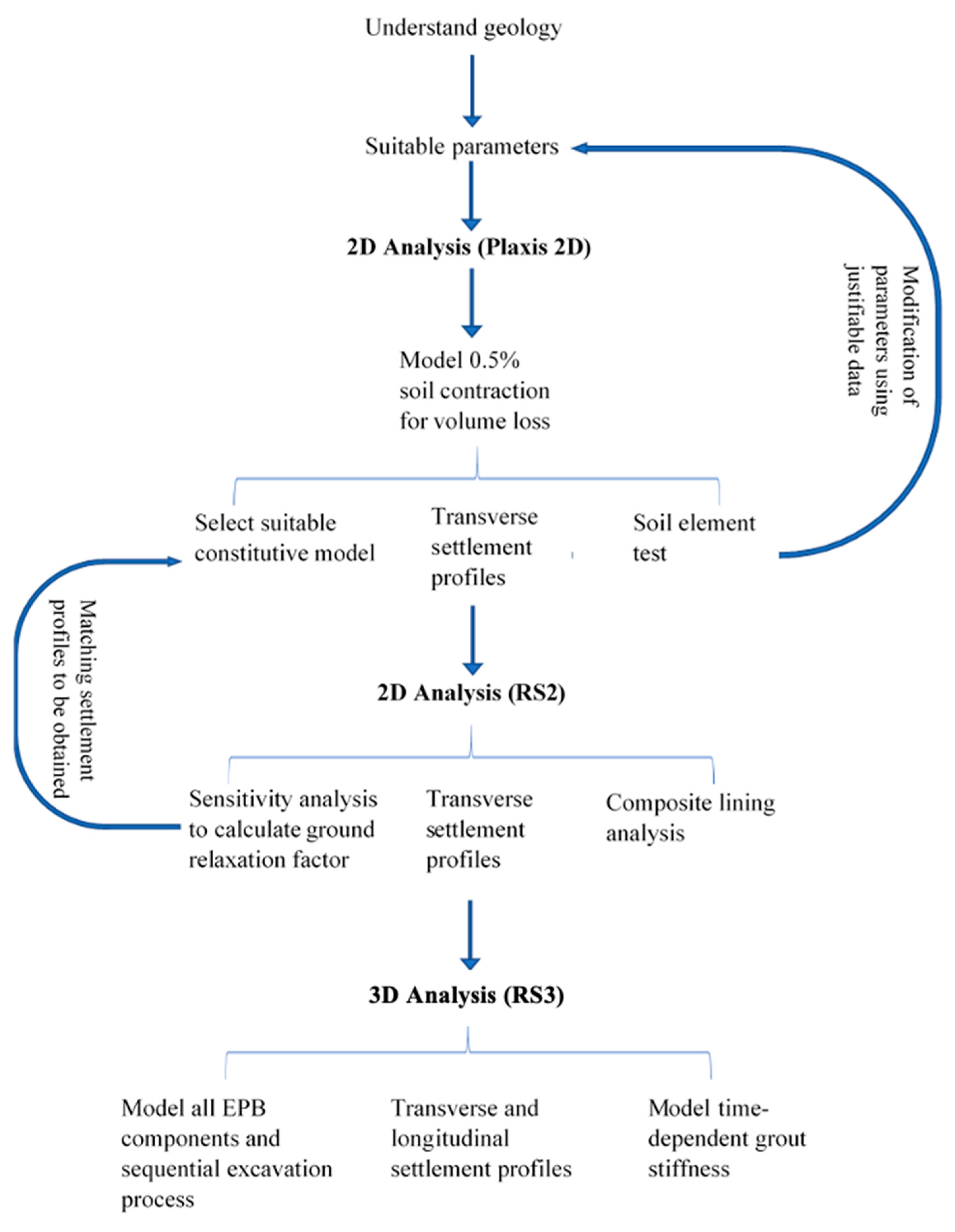
4. Numerical Analyses

The adopted approach in modelling tunnel excavation is summarised in Figure 5. It is based on an initial 2D analysis to provide quick, reliable results whilst having the benefit of testing the different constitutive models and calibrating parameters and performing a sensitivity analysis for volume loss. It is also used to compare the software before building geometrical complexity in RS3, at which stage, all the necessary components of an EPB excavation are modelled with a comparison of the longitudinal profiles across multiple constitutive models.
The initial PlAXIS2D model has three aims: firstly, to model and illustrate the volume loss around the shield due to conicity; secondly, to make a comparison of the basic and advanced constitutive models; and thirdly, to produce multiple transverse settlement profiles and conduct a lining deformation analysis. The latter ensures the validation of the choice of the constitutive model, but also provides a simple means of carrying out a diagnostic evaluation for the final choice of parameters before going forward to the 3D analysis. Each stage of the simulation signifies the passing of the TBM as follows in Figure 1b: stage 1 represents the initial state; stage 2 represents the TBM shield; stage 3 simulates the soil contraction phase; stage 4 simulates the normal applied grout pressure; and stage 5 represents the final lining installation. PLAXIS2D uses the contraction factor to model the volume loss around the shield, which fundamentally simulates the shield’s conicity. So, this is used for validation in conjunction with RS2, which uses the Lambda (λ) ground relaxation method to attain matching settlement profiles.

4.1. Model Input Parameters

4.1.1. Mohr–Coulomb

The strength values (φ and c) and elasticity values (E and v) are taken from Foster et al. (2021), who derived the values from [24] (Table 1). Regarding the elasticity, using the cross-borehole seismic method, the shear wave velocity parameters were calculated at multiple depths throughout the London Clay and converted to elasticity [25].

4.1.2. Hardening Soil and Hardening Soil with Small Strain

The parameters were initially established by [35] and tested for accuracy using Equation (1). They were found to be disproportionate to the corresponding elastic stiffness values that were adopted. Furthermore, the excavation depth for this paper is 50% greater than the ground model established by [35], and so they need to be reflective of this excavation depth and be changed accordingly (Table 2). All three stiffness parameters enable a non-linear failure criterion to be established during analysis.
A relationship between G0 and E0 was found in the study by [22], which relates to the elasticity parameters (Equation (1)). The E0 (maximal soil stiffness) is prescribed as 390 MPa after [24] The v is assumed to be constant at 0.2.
  E 0   > E u r   > E 50   G 0     E 0   2 1 + V
A corresponding γ0.7 value in relation to the E0 is adopted from Obrzud and Truty, 2018.

4.1.3. Other Parameters

The parameters for all the constitutive models were based on the findings from [35,36]. However, a critical analysis of the data with modifications was conducted to accommodate for the different geological conditions, mainly the depth. The HS model utilises the OCR value to approximate a more realistic K0 value [37]. It is common to expect an OCR value of 15 for London Clay at a 20–30 m depth [22]. This, therefore, produces a K0 value of 1.7 using Equation (2), which is moderately high but reasonable for London Clay.
K 0 =     K 0 N C ·   O C R sin ϕ  
However, any value of K0 > 1–1.5 is said to provide incorrect settlement predictions when using the HS/HSS model. According to [22], an OCR of 10 and a corresponding K0 of 1–1.2 was used.

4.2. Model Set-Up for 2D Analysis

4.2.1. Geometry Mesh and Boundary Conditions in 2D

The stratigraphy, as shown in Figure 4, was provided by Ramboll, UK. To simplify the numerical model shown in Figure 6, the Harwich formation unit (0.4 m thick) was grouped with the Lambeth group, and the alluvium deposits (0.4 m) were grouped with the River Terrace deposits. The tunnel invert is 42.5 m below ground level within the London Clay, with additional geometries found in Table 3. There are several empirical and analytical suggestions for calculating the domain size. Equation (3) from [38] relates the known overburden height and diameter to a plausible minimum width. At this width, no negligible deformation at the boundary should be encountered.
W = 2 D 1 + H D
The H/D ratio is 4.3, and this produces a width of 85 m. A simple sensitivity analysis was then used to assess this result’s validity by altering the width +/− 5 m. It was observed that 90 m was the optimum width as it did not encounter any edge effect anomalies in the results. This also correlates to the formula adopted by [5,20,39], suggesting the transverse distance to be 11 D (88 m).
Regarding the mesh, an eight-node graded triangular mesh was selected with the refining/coarsening option. This enables an optimal computational time-to-complexity ratio by coarsening the mesh in areas with low interest (RTD and Lambeth unit) and refining the mesh around the excavation perimeter and the made ground unit. For PLAXIS2D (Figure 6a), the side and base boundaries are set to automatic ‘fixities’. This fixes the base of the model in all directions and restrains movement to the vertical direction. For RS2 (Figure 6b), the same principle applies, so the top surface is ‘free’, and the base is fixed in the X/Y direction, with the side boundaries being fixed using roller boundaries.

Modelling EPBM Sequence

  • Segmental Lining and Shield
Concerning the material properties (Table 4), the weight (W) is factored in to minimise the uplift effects during construction. This is because PLAXIS2D and RS2 recognise that the soil elements represent the plate element’s volume (lining). Therefore, the weight (W) of the plate is needed to signify the additional weight of the plate (lining). For PLAXIS2D, the unit weight (γ) is multiplied by the plate thickness, whereas for RS2, the unit weight is directly inputted, and it is assumed to be 24 kN/m3 for both software tools. For PLAXIS2D, the axial stiffnesses (EA1 and EA2) are considered to have the same values as anisotropic stiffness is assumed. However, for RS2, the stiffness is prescribed by the Young’s modulus (E), which uses the same value as PLAXIS2D. The lining/shield is modelled elastically as a cylindrical shell without considering the lining jointing, as [5] reported minor surface settlement differences between continuous and jointed lining. The lining is activated (representing the shield) in the second stage with the corresponding contraction. It is then deactivated in the third stage, with reactivation in the last stage representing the final lining.
  • Grout pressure
The grout pressure is modelled as a uniform, normally distributed load that acts internally against the soil elements. This stage is implemented after the contraction has taken place. Due to the saturated undrained conditions, the pressure is calculated as the tunnel axis face pressure + 50 kPa [40]. RS2 provides the option of composite lining, thereby enabling the modification of the lining properties in a desired sequence of installation. The function will be used to model the primary lining, secondary lining and the hardened grout layer together. The grout layer will possess stiffness parameters from the 28-day hardened grout samples taken from [13]. In addition to the grout, a secondary lining (shotcrete) cast in situ is applied to the composite formation, as illustrated in Figure 4c, using the strength parameters taken from [41]. The composite lining parameters are shown in Table 5.
  • Volume loss
Modelling the volume loss as a result of ground relaxation becomes an integral part of simulating the shield conicity. However, the volume loss in London Clay is considered to be very small. PLAXIS2D uses the well-known contraction factor method, whereas RS2 uses the Lambda (λ) ground relaxation method. Ground relaxation is necessary during the EPB excavation. The optimum amount is determined when the in situ stresses are redistributed equally so that the lining takes the minimal amount of stress. It is essential for this component to be accurate because the vertical settlement will be dictated, to a certain extent, by this component. The contraction phase seen in Table 6 is assumed to be 0.5% as a function of the depth, soil mass stiffness and the data from the observed actual contraction values, varying between 0.2 and 1 for London Clay [42,43]. Using these data, a sensitivity analysis will be performed in RS2 to provide the ground relaxation factor needed to produce the same maximum displacement as seen in PLAXIS2D.
  • Contraction method
The contraction method proposed [44] in PLAXIS2D is the primary method of investigating the volume loss. The soil elements are removed, followed by the activation of the lining instantaneously (initial). This allows for the tunnel lining to displace freely as a shrinkage strain [45], which firstly experiences an uplift; however, this is counteracted slightly by applying the lining weight. The second phase simulates the actual contraction, whereby the soil mass contracts to the prescribed value (Table 6) as stress redistribution occurs.
  • Ground Relaxation Method
This ideology is also referred to as the convergence–confinement method (CCM), based on a theoretical framework derived from [46], which others [47,48,49,50,51] have developed further. The ground should naturally confine (relax) before the tunnel support is implemented to reduce the stress on the lining. The internal pressure (Pio) is reduced incrementally (Table 7) by a factor lambda (λ) until the same settlement profile seen from using the contraction factor in PLAXIS2D is produced. Therefore, there will be a corresponding relaxation factor for a given settlement profile using a 0.5% contraction.

4.3. Model Set-Up for 3D Analysis

The modelling process is split into several components, which need to be carefully considered, and a suitable number of stages need to be implemented to simulate the excavation process. The set-up of the 3D model closely follows aspects taken from [5,20,39] using Table 8, which can still be applied to this paper.

4.3.1. Geometry Mesh and Boundary Conditions in 3D

The 3D model is created using symmetry, with the vertical tunnel axis at the symmetry line. However, the model’s width is reduced to 45 m, but the height remains the same for stratigraphy reasons. The model’s length is prescribed to be 17.5 D (after [13]), representing 140 m (Figure 7a). RS3 allows for displacements to be staged, and so there are three basic model steps:
  • Firstly, the primary stage comprises ‘fixed’ displacements in the XY directions so that the virgin stress field is initiated with no excavations, with only the gravity loading activated. The displacements are also set to zero (free displacements) by the next stage. The latter is crucial because it ensures that the whole model is initially consolidated under gravity and that the settlement is only specified during the excavation.
  • In the second stage, the excavation (nulling) sections are activated.
  • The third stage and all proceeding stages follow the excavation sequence (Table 8).
A 12-node graded mesh is selected. The refinement option is used to a greater extent than the 2D analysis with a zone around the excavation perimeter. It utilises an element size of 0.6 m to densify the deformation zone (Figure 7b).

Modelling EPBM Sequence

  • Sequential excavation
The sequential excavation (Figure 7c) set-up is an essential component of 3D modelling. The sequential operation follows the repetitive procedure set out in Table 8. Each phase denoted as ‘n’ represents one excavated soil slice, which is deactivated during 1 stage of advancement for a total of 25 excavation stages. The n + 1 slice is the trapezoidal face pressure distribution application. The four preceding ring slices are then activated as the shield. The first ring outside of the shield is subject to the pressurised grout elements with direct contact to the soil elements concerning the annulus. A ring of the new lining (n-5, n-6, etc.) is installed immediately outside of the shield in the same stage. The elastic modulus increases gradually for each installed segment ring according to the hardening law set out by [14].
  • Segmental lining, shield and tail void
In RS3, it is assumed that the shield is cylindrical rather than conical, and the volume loss around the shield is not modelled for simplicity. In RS2, an induced load option utilising ground relaxation was possible. However, this function is not prevalent in RS3. Therefore, only the induced volume loss that is encountered far from the face and grout injections can be modelled.
The shield and lining can be distinguished with geometrical and strength accuracy. The shield is 8 m in length, representing four ring lengths, with each lining instalment corresponding to one ring length (Table 9). A complete composite lining model is analysed in 2D, but for 3D, only the primary lining and grout layer are considered. Regarding the tail void simulation, this is modelled as normal pressure internally to one ring length per stage, with the same calculation in the 2D analysis, and comes with its own set of assumptions. The grout’s pressure is directed towards the soil without considering that the distribution pressure will not be truly equal. The stage is represented only as a pressure that utilises the same stiffness values as the surrounding soil, when in reality, the stiffness of the fresh grout is greater [13].
  • Tail grout and time-dependent hardening stiffness
The ideal way to simulate the dynamic grout is to apply a time-dependant hardening factor that is influenced by the tunnel advance rate, which is assumed to be 18 m/day [5]. For an advancement rate of 18 m/day, it is assumed that the stiffness becomes constant after 14 days at 1 GPa (Shah et al., 2017) between stages 20 and 25. The increase in stiffness will be calculated exponentially between stages 1 and 20 from 0.1 MPa to 1 GPa and will be incorporated into the staged liner properties in RS3. The Poisson’s ratio will be kept constant at 0.25.
  • Face pressure
The face pressure is calculated using the density of the excavated muck mounting to 13 kN/m3 and the density of the material above [5]. Therefore, the face acts as a passive earth pressure that is needed to balance the active earth pressure directed at the face. The pressure is calculated at the crown and then at the invert, with an incremental pressure gradient being established as a trapezoidal pressure distribution.

5. Numerical Results

This section presents and evaluates the results with some meaningful reasoning towards the models’ responses to the excavation based on the numerical findings while comparing the 2D and 3D analyses.

5.1. PLAXIS2D and RS2 Analysis

The PLAXIS2D simulation revealed full settlement profiles (Figure 8a) for each of the constitutive models after the installation of the final lining, as well as a soil element test for calibration. It shows that the HS model closely fits the M-C model, predicting around 3 mm more settlement than the HSS model. The HSS illustrates a much flatter profile with more settlement around the site’s periphery and a comparatively shallower dip over the excavation. The sensitivity analysis (Figure 8b–d) shows the incremental reduction in the ground relaxation (GR) from 1 being an equal internal–external pressure. All models indicate a very similar settlement profile to PLAXIS2D, although they are less smooth, which may affect the mesh quality and gradation between the layers. This comparison shows the largest difference in the GR at 0.42 (Figure 8b) and 0.58 (Figure 8c), even though the settlement profiles appear to be very similar. Furthermore, the HSS model, which reveals the least settlement, requires an opposing large amount of relaxation. This highlights the dominant influence of increased stiffness with a low strain, hence less deformation.

5.1.1. RS2 Relaxation Analysis

Figure 9 shows the deformation pattern around the excavation. A K0 of 1.2 was used as it is more accurate for the London Clay at the considered depth. This, and a contraction factor of 0.5%, provided small surface settlements as expected.
  • Mohr–Coulomb (M-C) model
Generally, the crown displacement zone is narrow compared to the HS models (particularly HSS). Hence, the M-C settlement profile produces a greater Gaussian distribution above the axis. Figure 9a shows no displacement in the first stage, which should be the case because the pressure state is equal, and it is essential to calibrate it. All the deformation vectors are concentrated around the excavation periphery, are mainly orientated vertically and heave up in the invert.
  • Hardening Soil Standard (HS) model
The HS model results (Figure 9b) require a more incremental increase in relaxation between each stage; otherwise, computing would fail. A similar deformation pattern is seen, but it is more comprehensive, with the most deformation seen at the crown.
  • Hardening Soil with Small Strain (HSS) model
The HSS model results (Figure 9c) also require a more incremental increase in relaxation. More importantly, a similar deformation pattern between the final ground relaxation stage and the final lining model suggests that the necessary relaxation has occurred.

5.1.2. Lining Parametric Analysis

There is little effect on lining displacement between the composite lining (Comp) and the primary lining across all three constitutive models (Figure 10a). If anything, the composite lining shows slightly less displacement as anticipated. Nevertheless, it infers that the necessary ground relaxation has been established and that the full composite lining may not be necessary. There are some apparent anomalies for the M-C and HSS models (Figure 10b). Both show between −0.1 and 0.1 kNm for the composite lining compared to the primary lining, which possesses much greater bending moments. However, the HS model shows similar bending moments for both lining compositions. The bending moments for the HSS model seem more realistic compared to those obtained by [53] from the literature review, stating that 15–20 kN/m is typical for stiff soils because of ground relaxation.

5.2. RS3 Analysis

The 3D investigation can build upon all EPB components, including the added complexity that is associated with the applied trapezoidal face pressure distribution and time-dependent grout hardening. All three constitutive model representations show a general bullet-shaped excavation deformation zone with a tapered rear. This is a typical deformation pattern that is expected because it visibly shows the increased grout stiffness with advancement. The shield was assumed to be cylindrical, and therefore, the simulation was not subjected to shield volume loss. Hence, less settlement is witnessed (Figure 11). This impacts the overall maximum surface settlement ranging from 1 to 1.6 mm across all three constitutive models, which is less than expected and less than the transverse settlement profiles (Figure 8). The longitudinal profile shows some similar characteristics, whereby the most significant proportion of the settlement is seen between 7.5 tunnel radii in front of and behind the TBM, suggesting a 50–70 m zone of deformation influence across the three models, which is more expansive when compared to the literature [5,13]. The M-C and HS std. models’ displacements reach a constant value of approximately 10 tunnel radii behind the TBM face. In contrast, the HSS settlement profile develops a constant displacement by 7.5 tunnel radii.
  • Mohr–Coulomb (M-C) model
The M-C model (Figure 12a) is represented by the highest predicted maximum settlement, which correlates with the 2D analysis and illustrates deformation around the excavation, which is clearly due to face and grout pressure-induced volume loss. These EPB components can be extracted using the 2D contour plane generator in RS3. They show comparable deformation characteristics to the 2D analysis. The face pressure results show no inward deformation and appear to be reasonably stable. The shield is represented well, showing no inward displacement at the crown; however, the added shield weight parameter has not performed well, and an invert heave (0.0058 m) behaviour is evident. The grout pressure shows displacement in both the crown and invert, −0.0064 m and 0.012 m, respectively, which induces the necessary volume loss. The preceding rings employ the grout hardening behaviour, which evolves through time between stages 2 and 25, indicating a displacement reduction of approximately 50% in both the crown and invert. The final lining comprises full hardened grout (assumed to be 1 GPa), which shows minimal displacement in both the crown and invert and is 75% less than the fresh grout. However, long-term surface settlement is still prevalent towards the rear, which is expected to a degree, but counteracts the strengthened grout. One would expect the settlement rate to be reduced with time, which is not evident in Figure 11.
  • Hardening Soil Standard (HS) model
The HS model (Figure 12b) shows a similar excavation deformation zone to the M-C model. A gradual reduction in crown settlement from −0.0043 m to −0.00041 m can be observed with time. The HS model is represented as the intermediate predicted settlement, which differs from the 2D results. However, both the HS/HSS results show a slight heave (0.6 mm) at the XZ face of the domain, which is indicative of boundary effects due to the remobilisation of stresses at the boundary. So, these particular rings are ignored in the settlement profile. There is a considerable heave at the invert (0.015 m), which is unexpected, considering that this constitutive model works on the basis that there is a greater unload–reload stiffness. The grout pressure stage shows evidence of deformation, which encompasses a wider zone similar to 2D, so this has allowed for the necessary volume loss. As expected, it does not transfer as much to the surface compared to the M-C model.
  • Hardening Soil with Small Strain (HSS) model
The most notable anticipated feature of the HSS model (Figure 12c) is the reduced invert heave by about 50% compared to the HS model to a max displacement of 9 mm. This, unfortunately, is still 50% greater than the crown displacement. There is an anomalous area between 30 and 40 m behind the face, which shows a concentrated area of a more significant heave. Nevertheless, this is a negligible amount. Compared to the other models, the settlement profile appears to be flattened, which is a similar pattern seen in the 2D analysis. There is a more significant zone of displacement across the whole domain.

6. Discussion and Limitations

6.1. Two-Dimensional Analysis

One of the most striking aspects of the results is the more levelled curve for the HSS model (Figure 10a), which supports the concept of increased stiffness with smaller strains due to a stiff material, which transfers less deformation to the surface.
The M-C model can be seen to over-predict the vertical settlement due to the following: firstly, the stress levels being less than 50% of the ultimate strength [23], and secondly, when the elastic modulus is prescribed with a value that is smaller than the EUR (HS models). This is further exacerbated because it delivers a constant linear elastic zone until plastic deformation and will experience more strain.
Generally, the HS models take into account multiple features of soil behaviour. For example, the HSS model during a numerical investigation led by [28] was seen to fit closely with the observed Shanghai metro data from [54], which only saw a 0.54% settlement difference. In the 2D analysis, there is an unexpectedly large difference in the HSS settlement profiles compared to the HS profile, which seems peculiar considering that the only difference in the parameter input is the additional small-strain stiffness values γ0.7 and G0. This suggests that the small-strain stiffness plays a significant function in the deformation characteristics.
It is expected that the HS models concentrate and restrain the strain around the source of deformation as anticipated [22], and therefore may explain the lack of transferred soil deformation. The HSS model appears to pay more attention to the process of densification and has a higher association to densification than the expected stiffness. The shear strain modulus (G0) is obtained from a plausible E0 value derived from numerous London Clay tests undertaken by [24]. So, there is an assumption that their findings are credible, considering that most authors use these findings.
Each software indicated a much smaller amount of surface deformation with the HSS model, which is considered more realistic for the known behaviour of London Clay. As a result, it can be said that the choice of the constitutive model heavily dictates the prescribed GR factor needed to encourage the desired deformation. Regardless of this, it is still concluded that RS2 can be used to model the volume loss correctly based on a 0.5% contraction using PLAXIS2D as a proxy, which is a fundamental concept when trying to model an EPB excavation.

6.2. Three-Dimensional Analysis

There is a general continuity from 2D to 3D, with all components modelled, showing similar patterns as those in the literature. One concern, however, is that the overall surface settlement would have been maximised if the conicity could have been modelled more simply. A pattern is seen across the 2D and 3D analysis whereby the HSS and MC models deliver consistency with the least and most predicted settlements, respectively. Therefore, it can be inferred that the M-C model is likely to overestimate the deformation in this situation based on the theoretical understanding that the HS model reflects a true soil more closely.
There is an increase in a settlement between 30 and 40% at the shield tail across all three models, which is comparable to the estimations by [55],, who claimed that 40% of the settlement was attributable to the annulus. The face pressure initiates a deformation in front of the face (3.5D) of around 20% of the total settlement.
The standard HS model is now showing a less predicted settlement compared to 2D, being more relatable to the HSS model as hoped for. However, the standard model should still be used with caution because it is unable to comprehend high amplitudes of stiffness with small strains. One way around this could be to ensure that the three stiffness parameters are altered to reflect the whole domain’s strain levels rather than the soil tests. Further to this, it does not produce a complete elastic hysteresis, meaning that it cannot deform properly as anticipated, so it is not truly non-linear. However, there is still considerable deformation at the unloading boundaries (crown) where there are varying stiffnesses allowing for the initiation of high strain levels in the source region, which is more realistic [22].
Careful consideration of the HS model should be used when applying it to highly overconsolidated material such as London Clay, which was simulated using an OCR of 10. This is because the actual soil mass possesses noticeable anisotropy [24]. In contrast, the HS model was created in an isotropic framework [22] regarding the failure mechanism (uniform yielding surfaces), so it can be misleading in terms of giving variable settlement patterns in 2D and 3D. When looking at the longitudinal profile for the HSS, the model retains its structural integrity through time behind the shield with less long-term settlement [55]. This is supported by the findings obtained by [28], who reported the same vertical displacement after three months when the HSS model and observed data were compared. Simultaneously, the simpler M-C model shows a continued increasing settlement once the shield has passed, which can overestimate the soil deformation by up to 2.5–3 times more than the observations in some cases, according to [28].
There is substantial heave reported across all three models, namely the HS and M-C models, most likely as a response to shield uplift due to excavated ground unloading, which has then, in turn, counteracted the predicted crown settlements [5]. Thankfully, with the HSS model, it is evident that there is comparatively less heave around the shield, which is a better response to the greater Eur stiffness. This then allows for greater relaxation and corresponding crown displacement, whereas the M-C model is expected to overestimate heave because it utilises the same stiffness in both loading and unloading [5].
Concerning the EPB components, the high grout pressure simulation initiates a non-uniform stress distribution, as seen by [18], which reduces the predicted settlement accuracy [13]. This may also be a reason for the bending moments’ irregularities [53]. Regardless, this simulation is the closest applicable process in numerical modelling.

7. Concluding Remarks

Accurate numerical models for surface settlement predictions are needed to ensure safety and to limit conservative design, and they are subject to parameter selection and the choice of a constitutive model to best replicate the geological conditions. All EPB components were modelled with their corresponding influences on ground deformation through a complete, robust excavation process. The main limitation was the continuity between RS2 and RS3, whereby it was not feasible to account for ground relaxation in RS3, so the predictions were underestimated. However, the trends seen across the various models were consistent with each other.
The HS models are expected to represent reality, which was particularly true for the more advanced HSS model, which produces a settlement profile similar to the observations. The HS standard model is limited in that the failure mechanisms assume an isotropic failure mechanism in a heterogenous London Clay, which, in nature, includes high water pressure sand lenses and silt layers. However, a consideration of this would potentially overcomplicate the model. The HS standard model is less consistent across 2D and 3D analyses, but it appears to be more relatable to the HSS model during the 3D analysis, as anticipated. One noticeable feature of the HS model is the non-linearity of the strain deformation, which is more accountable for soils.
The 3D analysis shows that the HSS model produces a more laterally spread deformation zone with more emphasis on the settlement in front of the face whilst predicting the least settlement overall. The 2D analysis, which simulates all necessary volume loss, shows comparable HSS settlement predictions (4 mm) with the observed data from the site characterisation (Figure 3). It is generally expected that London Clay undergoes very little contraction in comparison to other soils. A small amount of surface settlement is expected, especially at an excavation depth of 34 m, so operating based on a 0.5% contraction factor was proven to be reasonable.
Both the 2D and 3D analyses revealed less invert heave, which supports the unload–reload stiffness theory behind the HSS mechanics well. Since it is not possible to simulate the shield conicity volume loss in an orthodox way, there are other potential options available. Firstly, it may be possible to model a low stiffness layer, which can be deformed, around the shield. However, this needs to be correlated to the correct expected contraction. Secondly, it may be possible to model an incredibly soft material, as stated in the gap, with steel elements in the shield. One can assume that the final convergence of the extrados is the maximum steering gap value. The M-C model is generically more suitable for rock deformation. As a result, it was seen in both the 2D and 3D analyses that the M-C model created overestimations of deformation.
Essentially, RS3 was able to model all the geometrical components using the available constitutive models, illustrating their responses to sequential tunnel excavation. In particular, the HSS model was capable of apprehending the cyclic loading–unloading of stiff soil during excavation. The shield conicity was not modelled for simplicity, and this would have provided extra expected settlement, producing a more conservative estimate. Regardless, similar settlement profiles were created. It should also be stated that in the presented research work, the effects of the grout’s time-dependent hardening clearly show a gradational increase in the lining strength with time.

Author Contributions

Conceptualization, C.P., R.S., R.M., J.T. and M.K.; methodology, J.T. and C.P.; software, J.T. and C.P.; validation, J.T., formal analysis, J.T.; investigation, C.P, J.T. and R.S.; resources, C.P. and R.M.; data curation, J.T. and C.P.; writing—original draft preparation, J.T. and C.P.; writing—review and editing, C.P. and M.K.; visualization, C.P.; supervision, C.P. and R.S.; project administration, C.P. All authors have read and agreed to the published version of the manuscript.

Funding

No funding available for this research.

Data Availability Statement

All data that have been generated and analysed is included in the presented research work.

Acknowledgments

The authors would like to thank Dimitrios Litsas and Panagiotis Sitarenios for their valuable feedback on this research work.

Conflicts of Interest

The authors declare no conflict of interest.

References

  1. Maidl, B.; Herrenknecht, M.; Maidl, U.; Wehrmeyer, G.; Sturge, D. Mechanised Shield Tunnelling; Wiley: Hoboken, NJ, USA, 2013. [Google Scholar]
  2. Paraskevopoulou, C.; Cornaro, A.; Admiraal, H.; Paraskevopoulou, A. Underground space and urban sustainability: An integrated approach to the city of the future. In Proceedings of the International Conference on Changing Cities IV: Spatial, Design, Landscape & Socio-Economic Dimensions, Chania, Greece, 24–29 June 2019; University of Thessaly: Volos, Greece, 2019. ISBN 978-960-99226-9-2. [Google Scholar]
  3. Paraskevopoulou, A.; Cornaro, A.; Paraskevopoulou, C. Underground Space and Street Art towards resilient urban environments. In Proceedings of the International Conference on Changing Cities IV: “Making our Cities Resilient in times of Pandemics”, Corfu, Greece, 20–25 June 2022. [Google Scholar]
  4. Carranza-Torres, C.; Rysdahl, B.; Kasim, M. 2013. On the elastic analysis of a circular lined tunnel considering the delayed installation of the support. Int. J. Rock Mech. Min. Sci. 2013, 61, 57–85. [Google Scholar] [CrossRef]
  5. Kavvadas, M.; Litsas, D.; Vazaios, I.; Fortsakis, P. Development of a 3D finite element model for shield EPB tunnelling. Tunn. Undergr. Space Technol. 2017, 65, 22–34. [Google Scholar] [CrossRef]
  6. Deng, H.-S.; Fu, H.-L.; Yue, S.; Huang, Z.; Zhao, Y.-Y. Ground loss model for analyzing shield tunneling-induced surface settlement along curve sections. Tunn. Undergr. Space Technol. 2022, 119, 104250. [Google Scholar] [CrossRef]
  7. Lou, P.; Li, Y.; Xiao, H.; Zhang, Z.; Lu, S. Influence of Small Radius Curve Shield Tunneling on Settlement of Ground Surface and Mechanical Properties of Surrounding Rock and Segment. Appl. Sci. 2022, 12, 9119. [Google Scholar] [CrossRef]
  8. Paraskevopoulou, C.; Benardos, A. Assessing the construction cost of tunnel projects. Tunn. Undergr. Space Technol. J. 2013, 38, 497–505. [Google Scholar] [CrossRef]
  9. Benardos, A.; Paraskevopoulou, C.; Diederichs, M. Assessing and benchmarking the construction cost of tunnels. In Proceedings of the 66th Canadian Geotechnical Conference, GeoMontreal on Geoscience for Sustainability, Montreal, QC, Canada, 29 September–3 October 2013. [Google Scholar]
  10. Paraskevopoulou, C.; Dallavalle, M.; Konstantis, S.; Spyridis, P.; Benardos, A. 2022. Assessing the Failure Potential of Tunnels and the Impacts on Cost Overruns and Project Delays. Tunn. Undergr. Space Technol. J. 2022, 123, 104443. [Google Scholar] [CrossRef]
  11. Rocscience.com. Learning Resources. 2020. Available online: https://www.rocscience.com/learning (accessed on 16 July 2020).
  12. PLAXIS 2018.1 Scientific Manual. Bentley, Advancing Infrastructure. Available online: https://www.cisec.cn/support/knowledgeBase/files/9C246B743FC5BC8C93BA3289873AC1B3636991439136189558.pdf (accessed on 9 August 2023).
  13. Shah, R.; Zhao, C.; Lavasan, A.A.; Peila, D.; Schanz, T.; Lucarelli, A. Influencing factors affecting the numerical simulation of the mechanized tunnel excavation using FEM and FDM techniques. Proceedings of EUROTUN 2017, IV International Conference on Computational Methods in Tunnelling and Subsurface Engineering, Innsbruck, Austria, 18–20 April 2017. [Google Scholar]
  14. Kasper, T.; Meschke, G. A numerical study of the effect of soil and grout material properties and cover depth in shield tunnelling. Comput. Geotech. 2006, 33, 234–247. [Google Scholar] [CrossRef]
  15. Clough, W.; Leca, E. EPB shield tunneling in mixed face conditions. ASCE J. Geotech. Geoenviron. Eng. 1993, 119, 1640–1656. [Google Scholar] [CrossRef]
  16. Herrenknecht, 2000. Available online: https://www.herrenknecht.com/en/products/productdetail/epb-shield/ (accessed on 10 July 2020).
  17. Ahmed, M.; Iskander, M. Evaluation of tunnel face stability by transparent soil models. Tunn. Undergr. Space Technol. 2012, 27, 101–110. [Google Scholar] [CrossRef]
  18. Koyama, Y. Present Status and technology of shield tunnelling method in Japan. Tunn. Undergr. Space Technol. 2003, 18, 145–159. [Google Scholar] [CrossRef]
  19. Lambrughi, A.; Medina, L.; Castellanza, R. Development and validation of a 3D numerical model for TBM-EPB mechanized excavations. Comput. Geotech. 2012, 40, 97–113. [Google Scholar] [CrossRef]
  20. Litsas, D.; Sitarenios, P.; Kavvadas, M. Influence of geometrical and operational machine characteristics on ground movements during EPB tunnelling. In Proceedings of the EUROTUN 2017, IV International Conference on Computational Methods in Tunnelling and Subsurface Engineering, Innsbruck, Austria, 18–20 April 2017. [Google Scholar]
  21. Koyama, Y.; Okano, N.; Shimizu, M.; Fujiki, I.; Yoneshima, K. In-situ measurement and consideration on shield tunnel in diluvium deposit. Proc. Tunn. Eng. 1995, 5, 385–390. (In Japanese) [Google Scholar]
  22. Obrzud, R.; Truty, A. The Hardening Soil Model—A Practical Guidebook; Z Soil.PC 100701 Report; Zace Services Ltd.: Preverenges, Switzerland, 2018. [Google Scholar]
  23. Tjie-Liong, G. Common Mistakes on the Application of PLAXIS2D in Analyzing Excavation Problems. Int. J. Appl. Eng. Res. 2014, 9, 8291–8311. [Google Scholar]
  24. Gasparre, A.; Nishimura, S.; Minh, N.; Coop, M.; Jardine, R. The stiffness of natural London Clay. Géotechnique 2007, 57, 33–47. [Google Scholar] [CrossRef]
  25. Hight, D.; Gasparre, A.; Nishimura, S.; Minh, N.; Jardine, R.; Coop, M. Characteristics of the London Clay from the Terminal 5 site at Heathrow Airport. Géotechnique 2007, 57, 3–18. [Google Scholar] [CrossRef]
  26. Schanz, T.; Vermeer, P.; Bonier, P. (Eds.) Formulation and verification of the Hardening Soil model. In Beyond 2000 in Computational Geotechnics; A.A Balkema, Rotterdam: Rotterdam, The Netherlands, 1999. [Google Scholar]
  27. Duncan, J.M.; Chang, C.Y. Nonlinear analysis of stress and strain in soils. J. Soil Mech. Found. Div. 1970, 96, 1629–1653. [Google Scholar] [CrossRef]
  28. Zakhem, A.; El Naggar, H. Effect of the Constitutive Material Model Employed on Predictions of the Behaviour of Earth Pressure Balance (EPB) Shield-Driven Tunnels. Transp. Geotech. 2019, 21, 100264. [Google Scholar] [CrossRef]
  29. Le, B.T.; Nguyen, T.T.T.; Divall, S.; Davies, M.C.R. A study on large volume losses induced by EBPM tunnelling in sandy soils. Tunn. Undergr. Space Technol. 2023, 132, 104847. [Google Scholar] [CrossRef]
  30. Benz, T. Small-Strain Stiffness of Soils and Its Numerical Consequences. Ph.D. Thesis, Universitat Sttutgart, Houston, TX, USA, 2007. [Google Scholar]
  31. Vakili, K.; Barciaga, T.; Lavasan, A.; Schanz, T. A practical approach to constitutive models for the analysis of geotechnical problems. In Proceedings of the 3rd International Symposium on Computational Geomechanics (ComGeo III), Krakow, Poland, 21–23 August 2013; pp. 738–749. [Google Scholar]
  32. Hardin, B.O.; Drnevich, V. Shear modulus and damping in soils: Design equations and curves. Geotech. Spec. Publ. 1972, 98, 667–692. [Google Scholar] [CrossRef]
  33. Sumbler, M.G. British Regional Geology: London and the Thames Valley, 4th ed.; British Geological Survey: London, UK, 1996. [Google Scholar]
  34. Royse, K.; de Freitas, M.; Burgess, W.; Cosgrove, J.; Ghail, R.; Gibbard, P.; King, C.; Lawrence, U.; Mortimore, R.; Owen, H.; et al. Geology of London, UK. Proc. Geol. Assoc. 2012, 123, 22–45. [Google Scholar] [CrossRef] [Green Version]
  35. Foster, J.; Paraskevopoulou, C.; Miller, R. Numerical Modelling and Sensitivity Analysis of the Interaction between Thameslink Rail Tunnels at King’s Cross and the Adjacent and Overlying Construction of Building S1. Geomech. Geoengin. Int. J. 2021, 16, 20–43. [Google Scholar] [CrossRef]
  36. O’Shea, O.; Paraskevopoulou, C.; Miller, R. Investigation of tunnel movement of the Thameslink Tunnels below Site S3 of King’s Cross Zone development. Geomech. Geoengin. Int. J. 2022, 7, 689–711. [Google Scholar] [CrossRef]
  37. Mayne, P.; Kulhawy, F. Ko−OCR relationship in soils. J. Geotech. Eng. Div. 1982, 108, 851–872. [Google Scholar] [CrossRef]
  38. Moller, S. Tunnel Induced Settlements and Structural Forces in Linings. Ph.D. Thesis, University of Stuttgart, Stuttgart, Germany, 2006. [Google Scholar]
  39. Sitarenios, P.; Litsas, D.; Kavvadas, M. The interplay of face support pressure and soil permeability on face stability in EPB tunneling. In Proceedings of the World Tunnel Congress (WTC), San Fransisco, CA, USA, 22–28 April 2016. [Google Scholar]
  40. Zhao, C.; Lavasan Alimardani, A.; Barciaga, T.; Zarev, V.; Datcheva, M.; Schanz, T. Model validation and calibration via back analysis for mechanized tunnel simulations—The Western Scheldt tunnel case. Comput. Geotech. 2015, 69, 601–614. [Google Scholar] [CrossRef]
  41. Bryne, L.; Ansell, A.; Holmgren, J. Laboratory testing of early age bond strength of shotcrete on hard rock. Tunn. Undergr. Space Technol. 2014, 41, 113–119. [Google Scholar] [CrossRef]
  42. Borghi, F. Soil Conditioning for Pipe-Jacking and Tunnelling; University of Cambridge: Cambridge, UK, 2006. [Google Scholar]
  43. Wongsaroj, J.; Borghi, F.; Mair, R. Effect of TBM driving parameters on ground surface movements: Channel Tunnel Rail Link Contract 220. Geotech. Asp. Undergr. Constr. Soft Ground 2006, 5, 335–341. [Google Scholar]
  44. Vermeer, P.A.; Brinkgreve, R. PLAXIS Version 5 Manual; Balkema, A.A., Ed.; Rotterdam: Rotterdam, The Netherlands, 1993. [Google Scholar]
  45. Khalid, M.; Kikumoto, M.; Cui, Y.; Kishida, K. The role of dilatancy in shallow overburden tunneling. Undergr. Space 2019, 4, 181–200. [Google Scholar] [CrossRef]
  46. Panet, M.; Guenot, A. Analysis of convergence behind theface of a tunnel. In Proceedings of the International Symposium, Tunnelling-82, Brighton, UK, 7–11 June 1982; pp. 187–204. [Google Scholar]
  47. Chern, J.C.; Shiao, F.Y.; Yu, C.W. An empirical safety criterion for tunnel construction. In Proceedings of the Regional Symposium on Sedimentary Rock Engineering, Taipei, Taiwan, 20–22 November 1998; pp. 222–227. [Google Scholar]
  48. Paraskevopoulou, C.; Diederichs, M.S.; Perras, M. Time-dependent rock masses and implications associated with tunnelling. In Proceedings of the EUROTUN 2017, IV International Conference on Computational Methods in Tunnelling and Subsurface Engineering, Innsbruck, Austria, 18–20 April 2017. [Google Scholar]
  49. Paraskevopoulou, C.; Diederichs, M. Analysis of time-dependent deformation in tunnels using the Convergence-Confinement Method. Tunn. Undergr. Space Technol. J. 2018, 71, 62–80. [Google Scholar] [CrossRef]
  50. Innocente, J.; Paraskevopoulou, C.; Diederichs, M.S. Estimating the long-term strength and time-to-failure of brittle rocks laboratory testing. Int. J. Rock Mech. Min. Sci. J. 2021, 147, 104900. [Google Scholar] [CrossRef]
  51. Innocente, J.; Paraskevopoulou, C.; Diederichs, M.S. Time-Dependent Model for Brittle Rocks Considering the Long-Term Strength Determined from Lab Data. Mining 2022, 2, 463–486. [Google Scholar] [CrossRef]
  52. Abaqus. ABAQUS/Standard Analysis User’s Manual; USA, 2011. Available online: http://130.149.89.49:2080/v6.11/pdf_books/CAE.pdf (accessed on 9 August 2023).
  53. Bilotta, E.; Russo, G. Internal Forces Arising in the Segmental Lining of an Earth Pressure Balance-Bored Tunnel. J. Geotech. Geoenviron. Eng. 2013, 139, 1765–1780. [Google Scholar] [CrossRef]
  54. Lee, K.; Ji, H.; Shen, C.; Liu, J.; Bai, T. Ground response to the construction of Shanghai metro tunnel-line 2. Soils Found. 1999, 39, 113–134. [Google Scholar] [CrossRef] [PubMed] [Green Version]
  55. Thewes, M.; Budach, C. Grouting of the annular gap in shield tunnelling—An important factor for minimisation of settlements and production performance. In Proceedings of the 35th ITA-AITES, World Tunnel Congress, Budapest, Syria, 23–28 May 2009. [Google Scholar]
Figure 1. (a) Schematic of the mechanics of an EPBM [16] and (b) simplified EPBM showing the simulation stages used for the numerical analysis herein.
Geosciences 13 00244 g001
Figure 2. (a) Applicability of constitutive models based on the soil type taken from the Z_soil manual from [22]; note, ‘Std’ is ‘standard’. (b) Stress–strain curves of Mohr–Coulomb model compared to real soil non-linear behaviour (modified from [23]). (c) Stress–strain curves of hardening–softening model showing the three different stiffness regimes (modified from [23]).
Geosciences 13 00244 g002
Figure 3. Monitoring points and observed settlement for the area under investigation (data provide by Ramboll, UK).
Geosciences 13 00244 g003
Figure 4. (a) Northwest–southeast cross section of the London Basin (after [34]). (b) The ‘Palaeogene and Neogene’ unit representing the whole stratigraphic column of interest. (c) Ground model illustrating the tunnel specification and the geology for the numerical simulation.
Geosciences 13 00244 g004
Figure 5. Flow chart showing the methodology used in this analysis.
Geosciences 13 00244 g005
Figure 6. Two-dimensional model set-up for (a) PlLAXIS2D and (b) RS2.
Geosciences 13 00244 g006
Figure 7. Three-dimensional model set-up for RS3 analysis. (a) Tunnel domain and geometry, (b) mesh set-up and (c) sequential excavation.
Geosciences 13 00244 g007
Figure 8. (a) PLAXIS2D settlement profiles for each constitutive model based on 0.5% contraction and RS2 sensitivity analysis to calculate ground relaxation factor (GR) for (b) M-C, (c) HS and (d) HSS constitutive models.
Geosciences 13 00244 g008
Figure 9. RS2 results showing crown and invert displacement during ground relaxation for (a) M-C, (b) HS and (c) HSS constitutive models.
Geosciences 13 00244 g009
Figure 10. (a) Liner displacement comparison between primary lining and composite lining illustrating not much difference, and (b) evidence of large difference in bending moments between the composite and primary linings with respect to the M-C and HSS constitutive models.
Geosciences 13 00244 g010
Figure 11. Longitudinal settlement profile for each constitutive model after 25 stages.
Geosciences 13 00244 g011
Figure 12. Displacement profiles for each constitutive model after 25 stages: (a) M-C, (b) HS and (c) HSS constitutive models.
Geosciences 13 00244 g012
Table 1. M-C parameters for the numerical model (from [35]), (*) represents data from different sources.
Made Ground (M-C) London Clay (M-C)
General
Properties
γDRY
(17 kN/m3)
γSAT
(19 kN/m3)
Drained General
Properties
γDRY
(18 kN/m3)
γSAT
(20 kN/m3)
Undrained (A)
K = 1.95 × 10⁻⁵
StrengthStiffness StrengthStiffness
ParametersValueParametersValue ParametersValueParametersValue
φ30°E10,000 φ23° 100,000
c0 kPaν (nu)0.2 c5 kPa 0.2
InterfaceInitial InterfaceInitial
Fully permeableRINTER—rigid (1)K0—0.5–1.2 Semi-permeableRINTER—rigid (0.7)K0—0.609–1.2
   
RTD (M-C) Lambeth group (M-C)
General
Properties
γDRY
(17 kN/m3)
γSAT
(19 kN/m3)
Drained General
Properties
γDRY
(17 kN/m3)
γSAT
(19 kN/m3)
Drained
StrengthStiffness StrengthStiffness
ParametersValueParametersValue ParametersValueParametersValue
φ30°E25,000 * φ23°E45,000
c0 kPaν(nu)0.2 c0 kPaν (nu)0.2
InterfaceInitial InterfaceInitial
Fully permeableRINTER—rigid (1)K0—0.45–1.2 ImpermeableRINTER—rigid (1)K0—0.609–1.2
Table 2. HS and HSS parameters for the numerical model (from [24,35]), (*) represents data from different sources.
London Clay (HS/HSS)
General propertiesγDRY
(18 kN/m3)
γSAT
(20 kN/m3)
Undrained (A)
K = 1.95 × 10 −5
StrengthStiffness
ParametersValueParametersValue
φ23° E 50 r e f 40,000 kPa
c5 kPa E u R r e f 120,000 kPa
OCR stress1–15 E o e d r e f 35,000 kPa
M (power)0.9
Advanced StrengthAdvanced Stiffness
RF (Failure ratio)0.9v (nu)0.2
Tensile strength5 kPa *Pref100 kPa
K00.609—1.2
Small strain (HSS only)Interface
γ0.73 × 10⁻⁴RINTER0.7
G0162,000 kPaInterfaceImpermeable
RS2—additional parameters
Plimit10 kPa *Dilation angle
Table 3. Geometrical dimensions used for PLAXIS2D and RS2.
Geometrical ComponentsDimensions
External box90 m (width), 55 m (depth)
Overburden height34.5 m
Tunnel diameter8 m extrados, internal (7.3 m)
Shield/primary lining0.35 m thick
Secondary lining0.25 m thick
Grout width0.1 m thick
Table 4. Lining parameters for the primary lining (plate elements), obtained from [35].
Primary Lining
PLAXIS2DRS2
Lining width0.35 mLining width0.35 m
Poisson’s ratio (v)0.2Poisson’s ratio (v)0.2
EA 1 (in-plane)3.60 × 10⁶ kPaE’3.60 × 10⁶ kPa
EA 2 (out-of-plane)3.60 × 10⁶ kPaUnit weight24 kN/m3
EI (flexural rigidity)2.70 × 10⁴ kPa
W8.4 kN/m3
Table 5. Composite lining parameters for RS2 used for the parametric study.
ParametersPrimary LiningSecondary Lining
[41]
Grout after 28 Days
[13]
Units
BehaviourPlasticplasticPlastic
Unit weight242424kN/m3
Modulus of elasticity36361.5–2.5GPA
Poisson’s ratio0.150.150.3
Compressive strength45671.5–2MPa
Table 6. PLAXIS2D steps of the construction process, showing 0.5% contraction.
StagePhaseConstruction StepsModel StepsJustification/Comments
Geosciences 13 00244 i001
1 (Pre-excavation)--Initial stress conditions in equilibrium across all layers
-Select ignore undrained behaviour
Visualise original conditions to reference displacement change.
Geosciences 13 00244 i0022 (Excavation)Excavation-Reset tunnel displacements to 0
-Deactivate soil unit inside tunnel and set deconfinement of clusters to 100%
-Set water conditions to dry in tunnel volume
Deactivating the soil only effects the soil strength and stresses; therefore, setting the water condition to 0 is needed to deactivate the water pressure.
A 100% deconfinement means there is zero internal support pressure, which allows for soil convergence.
Geosciences 13 00244 i0033 (Construction)Lining-Activate tunnel lining as plate elements with the concrete segment material properties
-Activate negative interface
Lining is constructed under the protection of the shield so there is no soil contraction yet.
The negative interface creates a soil–structure interaction.
Geosciences 13 00244 i0044 (Construction)Contraction-Select all segment plate elements and activate contraction (Cref = 0.5%)A Cref of 0.5% is acceptable for excavation in London Clay, allowing for stress re-distribution.
The liner contraction will be 0.25% because the actual strain to the lining is half of the applied contraction.
Geosciences 13 00244 i0055 (Construction)Grouting-Reset displacements to zero is NOT selected
-Deactivate lining, interface and contraction
-Activate water conditions to user-defined conditions
(grout pressure) −387 kPa
This sustains the previous contractions before grouting.
The deactivation of plates allows for the grout pressure to transmit from the tunnel axis outwards to the soil interface as an equal pressure distribution.
The calculated grout pressure can be exerted to the annular gap in the contraction area.
Geosciences 13 00244 i0066 (Construction)Final lining-Do not reset displacements to zero
-Set tunnel volume to dry
-Re-activate lining plates and interface
This allows for any grout contraction.
The effects of the grout pressure on the contraction have already been accounted for.
The lining reactivation concludes the final stage.
Table 7. RS2 steps for construction process, showing ground relaxation phase.
StagePhaseConstruction StepsModel StepsJustification/Comments
Geosciences 13 00244 i007
1 (Pre-excavation)-Initial stress condition ignores undrained behaviourObserve initial stable conditions.
GR 1 (Po = Pi)2ExcavationSoil unit inside the tunnel is deactivated at this stage
Geosciences 13 00244 i008
3 (Construction)Incremental
Ground
Relaxation
Staged increase in ground relaxation for both the M-C and HS/HSS models based on the sensitivity analysis

Decrease in GR of 0.1 per stage for M-C model, with smaller increments of 0.05 for the more sensitive HS/HSS model
RS2 offers the ground relaxation method to simulate volume loss, which is performed in progressive stages with the aim of matching the surface settlement profiles seen in PLAXIS2D.
A GR factor will be established, which will produce the same settlement profile seen in PLAXIS2D at a contraction factor of 0.5%.
The GR method already takes the grout pressure into account, so there is no added stage for this.
Geosciences 13 00244 i0094 (Construction)Final LiningThe final lining is activated once sufficient ground relaxation has taken place and negative interface is activatedThe final lining will take on a much smaller loading pressure because the ground has been given time to relax, so the lining stability is optimised.
Table 8. Case study comparison in relation to the modelling of the EPB components and sequential excavation, which is used in this analysis.
Model Components[20][39][5]
Constitutive modelModified Cam-Clay—plastic and Mohr–Coulomb failure (elastic–plastic)Modified Cam-ClayLinear elastic–perfectly plastic Mohr–Coulomb failure.
GeologyAll share similar geological conditions in soft to stiff clayey soils; ground water was assumed at the surface with saturated undrained conditions with low permeabilities (10–8 m/s)
GeometryShallow 10 m D tunnel symmetrical half-model across axis8 m D tunnel symmetrical vertical plane aligned across tunnel axisTunnel D—10 m; symmetry not used because transverse lining joints were used.
BoundariesHorizontal profile—11D
Longitudinal profile—13D (H/D = 1.5); overburden height at 15 m; free surface at top and fixed sides
Horizontal profile—50 m
Vertical (depth)—56 m
Longitudinal profile—5D (40 m)
H/D = 2.5—overburden height (20 m)
H/D = 2—overburden height (20 m).
Longitudinal profile—13D.
Horizontal profile—11D.
MeshAdaptive meshing technique (ALE)—resets the deformed peripheral mesh around the face back to its original structure with no interference on the stress–strain fieldDense discretisation around excavation, with coarseness increasing towards the boundaries 
EPB shieldTapered shield for steering gap (4 cm); modelled with appropriate stiffness and weightStiff shell elements to signify the shield 
Face pressureThe applied pressure varies linearly across the face height, acting as a trapezium pressure distribution; the assumed bulk density of the applied muck was 13 kN/m3Supported by a redefined pressure accompanied by one slice of unsupported excavated material (simulates overcut)-trapezoidal support pressure; the assumed bulk density for the muck was 15 kN/m3Assumption of linear variation of earth pressure (Ka) with depth using a bulk density of muck equal to 13 kN/m3 and a reference pressure that is approximately equal to 50% of the horizontal stress.
BackfillingPressurised grout elements modelled as interface elements, which comply with an ‘exponential pressure overclosure’ relationship; annular gap—grout hardening Modelled using 8-node solid elements. Time hardening grout from Kasper and Meshke, 2006 was used for the proposed curve. The grout injection pressure was varied (100–400 kPa).
LiningModelled as continuous shellModelled as continuous shellFocus on segmental lining with inter-plate joints. Analysis on joint interaction and stress at interface using JOINTC, which allows for small rotations and internal stiffness [52]. A staggered configuration aimed to increase stiffness.
 Lining was modelled as linear–elastic due to lining stresses being minimal [20]. The components are as follows:
Sequential excavation pattern1. Excavation slice denoted as ‘n’, measuring 1 ring length with an advancement of 1.5 m;
2. ‘n + 1’ is the excavated face that receives the direct support pressure;
3. Slice ‘n-7’ is the first ring outside the shield at the rear–soil interaction activated at this point;
4. ‘n-6’ is the next slice to be activated;
5. Stiffness increases gradually from slices ‘n-7’ to ‘n-8’ and go on to replicate the grout hardening process [14].
6. Advancement rate between 15 and 18 m/day.
Table 9. Geometrical components of the 3D model; (*) represents the time-dependent stiffness evolution.
ParametersTBM ShieldPrimary LiningGrout
[13]
Units
BehaviourElasticElasticElastic
Unit weight242424kN/m3
Modulus of elasticity209360.1–1000 *MPa
Poisson’s ratio0.150.150.3
Compressive strength 401.5MPa
Geometrical componentsDimensions
(Symmetry half model)
External box45 m (width), 140 m (length) and 55 m (depth)
Overburden height34.5 m
Tunnel diameter8 m extrados, internal (7.3 m)
Shield thickness0.1 m
Shield length8 m (4 ring lengths)
Primary lining0.35 m thick
Grout width0.1 m thick
Disclaimer/Publisher’s Note: The statements, opinions and data contained in all publications are solely those of the individual author(s) and contributor(s) and not of MDPI and/or the editor(s). MDPI and/or the editor(s) disclaim responsibility for any injury to people or property resulting from any ideas, methods, instructions or products referred to in the content.

