Article

Implementation of a Cascade Fault Tolerant Control and Fault Diagnosis Design for a Modular Power Supply

1
High Institute of Applied Sciences and Technology, University of Kairouan, Kairouan 3100, Tunisia
2
Laboratory of Analysis, Conception and Control of Systems LR11ES20, Université de Tunis El Manar, Ecole Nationale d’Ingénieurs de Tunis, Tunis 1002, Tunisia
3
Escuela de Ingeniería de Vitoria, Universidad del País Vasco, Nieves Cano 12, 01006 Vitoria, Spain
*
Author to whom correspondence should be addressed.
Actuators 2023, 12(3), 135; https://doi.org/10.3390/act12030135
Submission received: 18 February 2023 / Revised: 10 March 2023 / Accepted: 20 March 2023 / Published: 22 March 2023
(This article belongs to the Special Issue Actuators in 2022)

Abstract

:
The main objective of this research work was to develop reliable and intelligent power sources for the future. To achieve this objective, a modular stand-alone solar energy-based direct current (DC) power supply was designed and implemented. The converter topology used is a two-stage interleaved boost converter, which is monitored in closed loop. The diagnosis method is based on analytic redundancy relations (ARRs) deduced from the bond graph (BG) model, which can be used to detect the failures of power switches, sensors, and discrete components such as the output capacitor. The proposed supervision scheme including a passive fault-tolerant cascade proportional integral sliding mode control (PI-SMC) for the two-stage boost converter connected to a solar panel is suitable for real applications. Most model-based diagnosis approaches for power converters typically deal with open circuit and short circuit faults, but the proposed method offers the advantage of detecting the failures of other vital components. Practical experiments on a newly designed and constructed prototype, along with simulations under PSIM software, confirm the efficiency of the control scheme and the successful recovery of a faulty stage by manual isolation. In future work, the automation of this reconfiguration task could be based on the successful simulation results of the diagnosis method.

1. Introduction

Power converters play a crucial role in supplying direct or alternating current to actuators. Therefore, ensuring the reliability of power supplies is of utmost importance. Interleaved boost converters (IBCs) can be used as an alternative to increase reduced voltage levels, and they have proven to be more reliable than conventional boost converters [
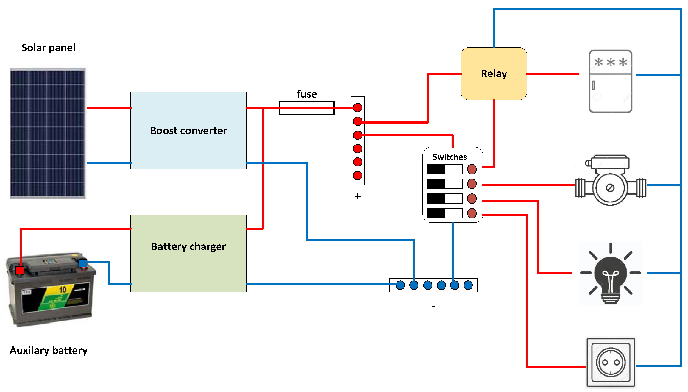
1]. In stand-alone applications that rely on renewable energy sources, there is high demand for 12 VDC and 24 VDC. Modular power supplies, which utilize free and clean solar energy, can act as secondary power sources to relieve powertrain systems in cars, especially for vehicles such as camping-cars, which require a reliable and non-polluting energy source. Camping-car owners who seek complete freedom in their travels, without the need for charging stations, often require autonomy in electricity. The photovoltaic (PV) panels of 6 VDC and 12 VDC are commonly used, and finding reliable and modular voltage doublers is essential. The reliability of such doublers is described as follows: if one stage fails, another can take over, ensuring the continuity of service. The reader can refer to [2] to understand the differences between various DC-DC converters like buck, buck-boost, SEPIC, and flyback, as well as their applications in photovoltaic systems, array configurations, advanced maximum power point tracking (MPPT) methods, and comparisons in terms of hardware complexity, cost, and efficiency. The use of interleaved DC converters is gaining interest from both industrialists and researchers in the power electronics and converters field. These converters provide a relatively low-input current ripple, making them more attractive.
The control of power converters is a well-researched area with the aim of optimizing the system and maintaining its efficiency despite parameter variations and external disturbances. Due to the strong nonlinearity of the PV panel and power converter, nonlinear controllers are often used to address this challenge. Several control techniques have been proposed and tested, such as the incremental Conductance Maximum Power Point Tracking (InC MPPT) algorithm [3], proportional–integral–derivative control (PID), flatness theory [4], and passivity-based control [5]. While these methods have been effective, practical implementation remains a significant task. One promising approach is that of sliding mode control (SMC), a robust and widely used controller in various fields including power converters in photovoltaic energy (see, e.g., [6,7,8] and the references therein). Several papers have reported on the effectiveness of SMC, with applications ranging from flyback-based PV systems [9] to bidirectional DC converters [10]. To increase the efficiency, SMC is often consolidated with other methods such as PI control [11]. A novel direct sliding mode controller (DSMC) has also been proposed to minimize the use of unreliable DC-link capacitors in large electrolytic capacitors used in grid-connected and stand-alone photovoltaic applications [10].
A fast fault diagnosis and fault-tolerant method for DC–DC converters is mandatory, even though it is possible to enhance the structure of the IBC to reduce stress on power components as seen in [12]. The fault diagnostic algorithm comprises two parts: fault detection and fault identification. Model-based methods are prevalent and attractive for power converters, using the analytic knowledge of the system since there is generally a certain level of knowledge about parameters allowing for the construction of state observers, parity equations, or residual generation. Fault-tolerant control (FTC) establishes the process’s reconfiguration to avoid shutdown. It can be active or passive. Active techniques reconfigure the control parameters in the presence of a fault but passive ones consider that possible system failures are known. The controller is thus developed to cover a set of specified faults [13]. When the system has adequate sensors, it is possible to analyze the inductance voltage and deduce the non-symmetry of the stage and apply a fault-tolerant control to recover the faulty component [14,15]. However, most diagnosis methods use the inductance current itself. Based on the switching frequency, it is possible to analyze the harmonic components, and a system reconfiguration is applied to reduce input current ripples by only allowing the healthy stages [16]. Observers are also a considerable approach in the case of weak sensor presence, regardless of whether this is intended or not [17,18,19,20]. Based on the simplicity and robustness of immersion and invariant (I&I) theory, I&I observers are proposed in [17] and adopted for residual generation to detect switch open failure. In this case, there was a need to adapt the threshold to eliminate false alarms. Salman et al. [18] proposed a generalized PI observer to detect open switch faults. Extensive research has been performed on the open circuit fault [17,18,21,22,23,24]. A limited number of papers are dealing with sensor faults [18], short-circuit faults [21,23,25], and capacitor faults, which are an important source of faults in a power converter (capacitor 30%, printed circuit board 26%, and semiconductor 21%) [26].
Faults affecting power capacitors are varied, and most of them are caused by switching semiconductors. Moreover, the kind of material has a great effect on the reliability of capacitors and semiconductors [27]. The detection of power capacitor faults can be associated with artificial intelligence (AI). The authors in [28] used deep learning associated with fuzzy logic and [29] used a convolutional neural network combined with the chaotic synchronization. The proposed methods have good results but the complexity of implementing these methods in embedded systems remains a real challenge.
Rule-based fault monitoring and location methods are imperfect and inflexible as they use simple predictive rules to identify the possible causes of system failures. Machine learning methods have been successfully applied to PV systems [
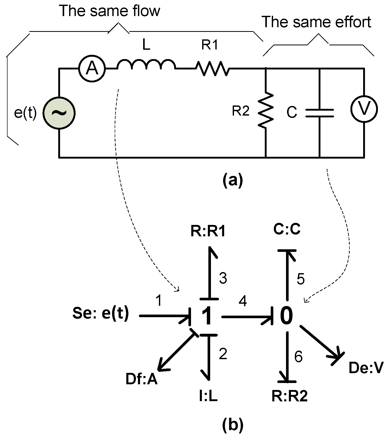
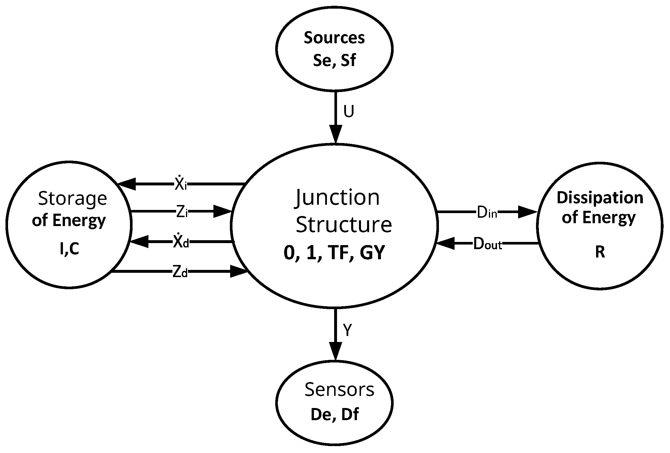
30], but these require a historical database to be effective. Model-based fault monitoring and diagnosis methods are based on the physical system’s behavior and structure, and use a model to represent a large amount of information about its structure, function, and behavior. The bond graph (BG) formalism provides several advantages, including the ability to deduce cause–effect relationships and study causality at the system level. This method is attractive as it can detect various types of failures, although it requires an increased number of sensors. It can integrate artificial intelligence, such as Bayesian networks and reliability failure rates, and has been used for modeling, analysis, control, and monitoring in the power converter field [31].
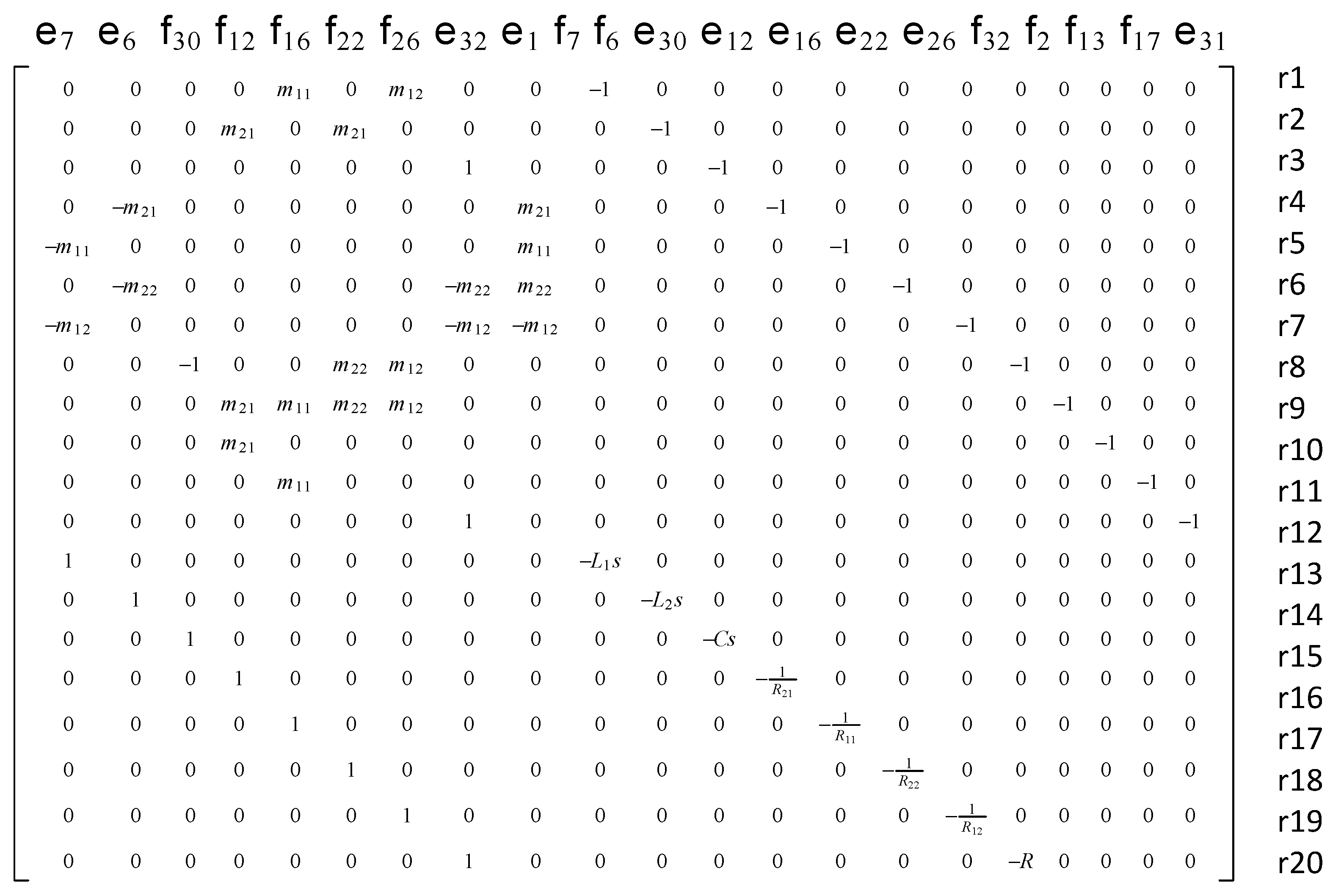
Analytic redundancy relations (ARRs) is a model-based method used for fault diagnosis. The method involves developing the mathematical models of a system and using them to detect and isolate the faults that occur in the system. The basic idea behind ARR is that a system has a number of redundant measurements, and faults can be detected by comparing the measurements with the predictions of the model. The principle of fault detection and isolation (FDI) using ARRs deduced from the BG model consists of establishing a fault or a matrix signature, as shown in Table [32]. This method has been applied in real complex systems such as steam generator process [33,34] but applications in the field of power converters are limited. These relations can be symbolically generated and are therefore suitable for computer implementation. In [35], a model builder software for fault detection and identification was developed and implemented for thermofluid processes. The fault diagnosis of an electric scooter is carried out using ARR and modified analytic redundancy relations (MARRs) in [36,37]. MARRs are derived to model the multiplicative faults of non-parametric components, such as actuators and sensors, by introducing efficiency factors.
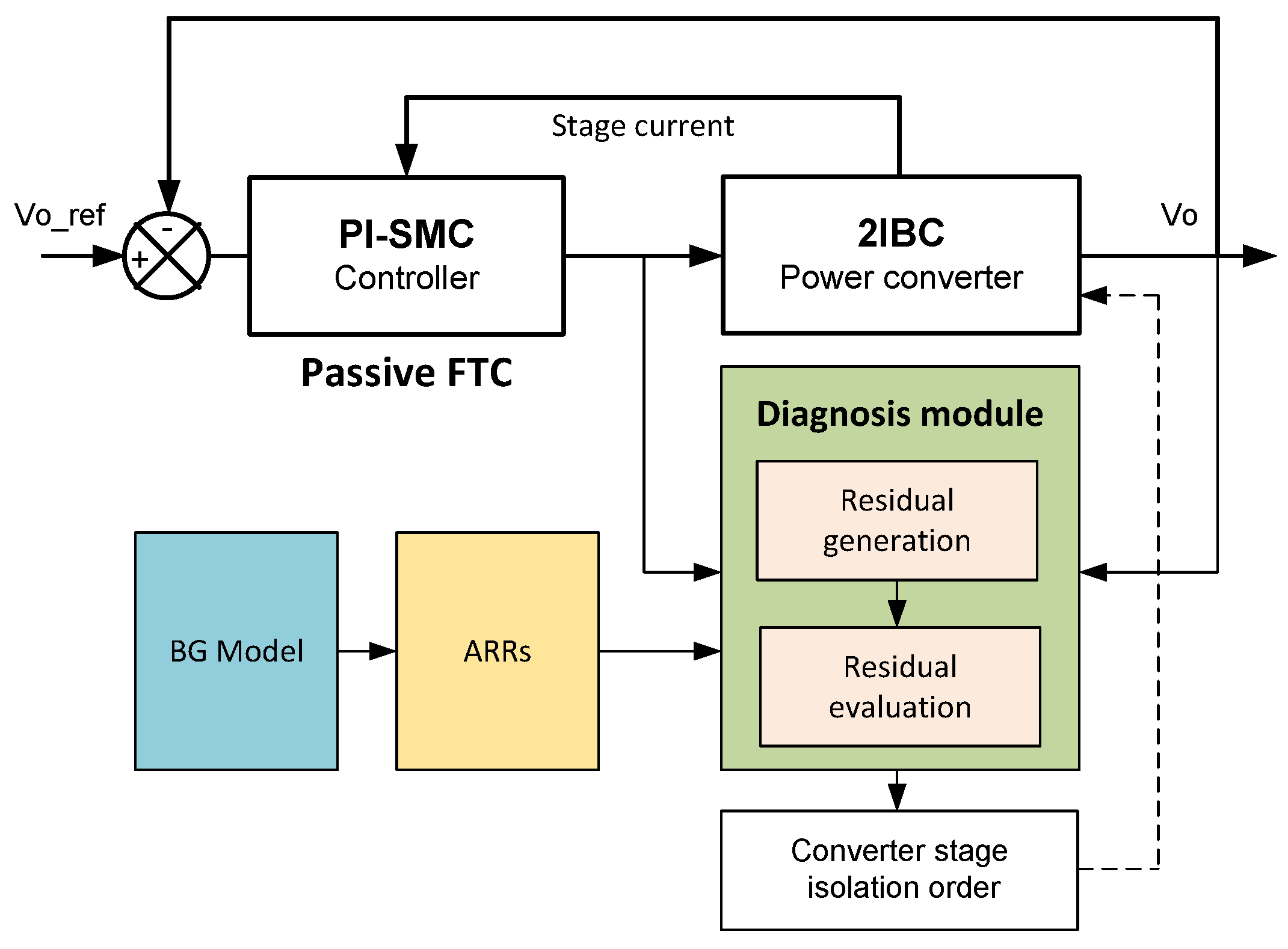
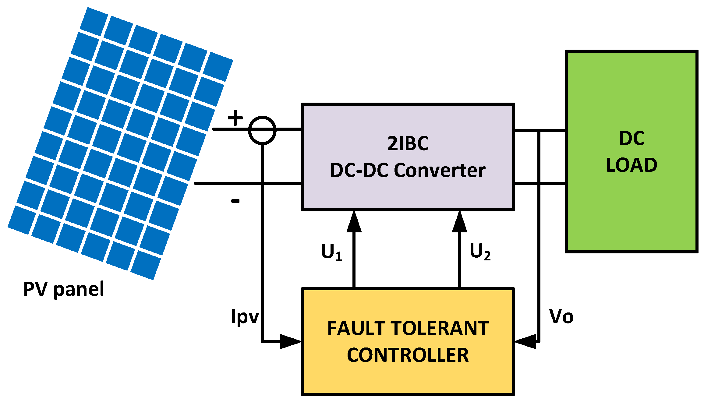
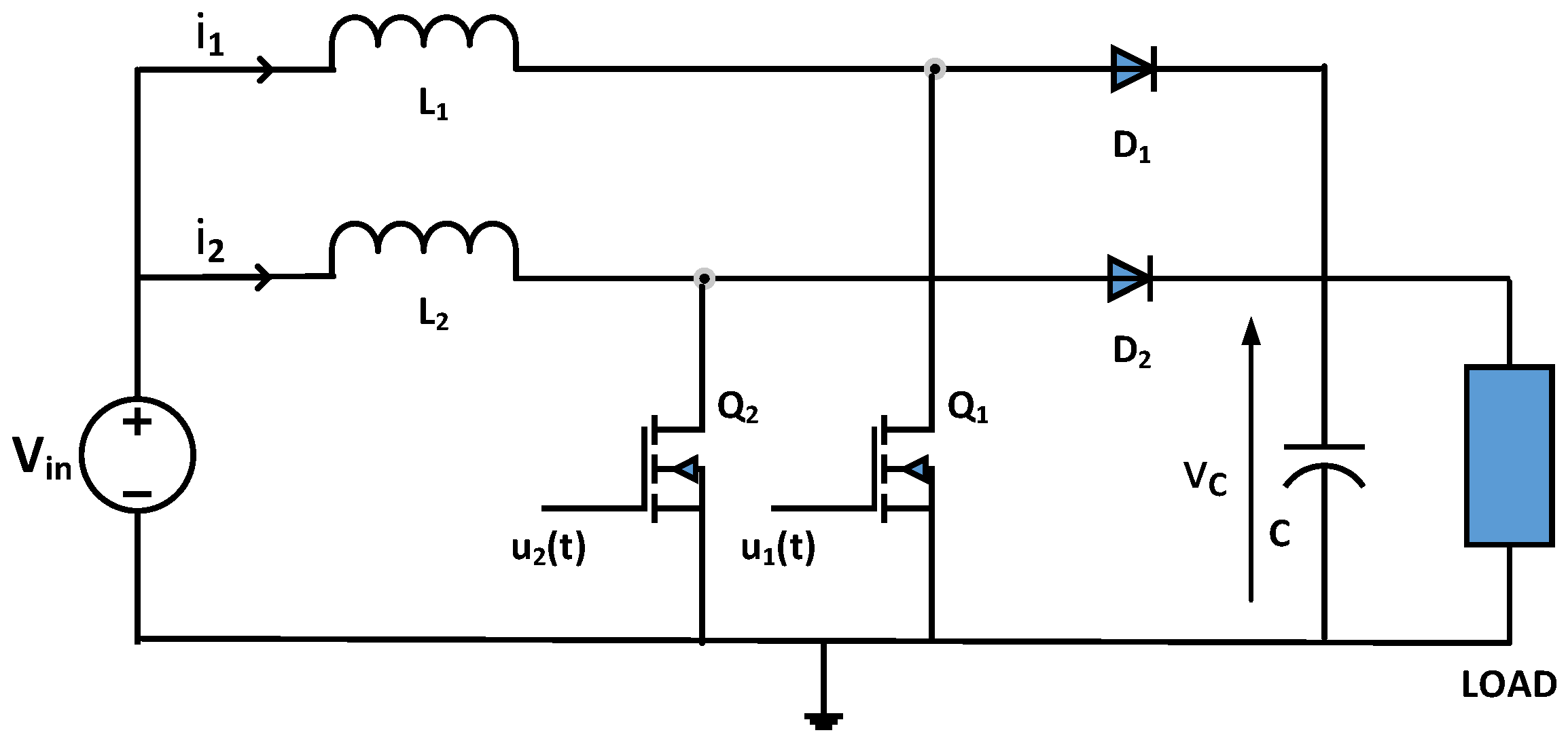
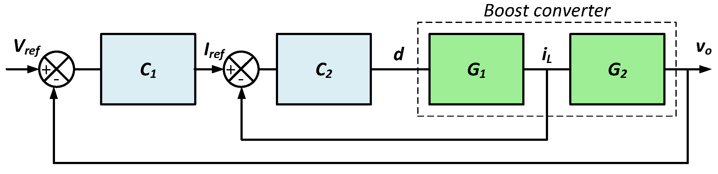
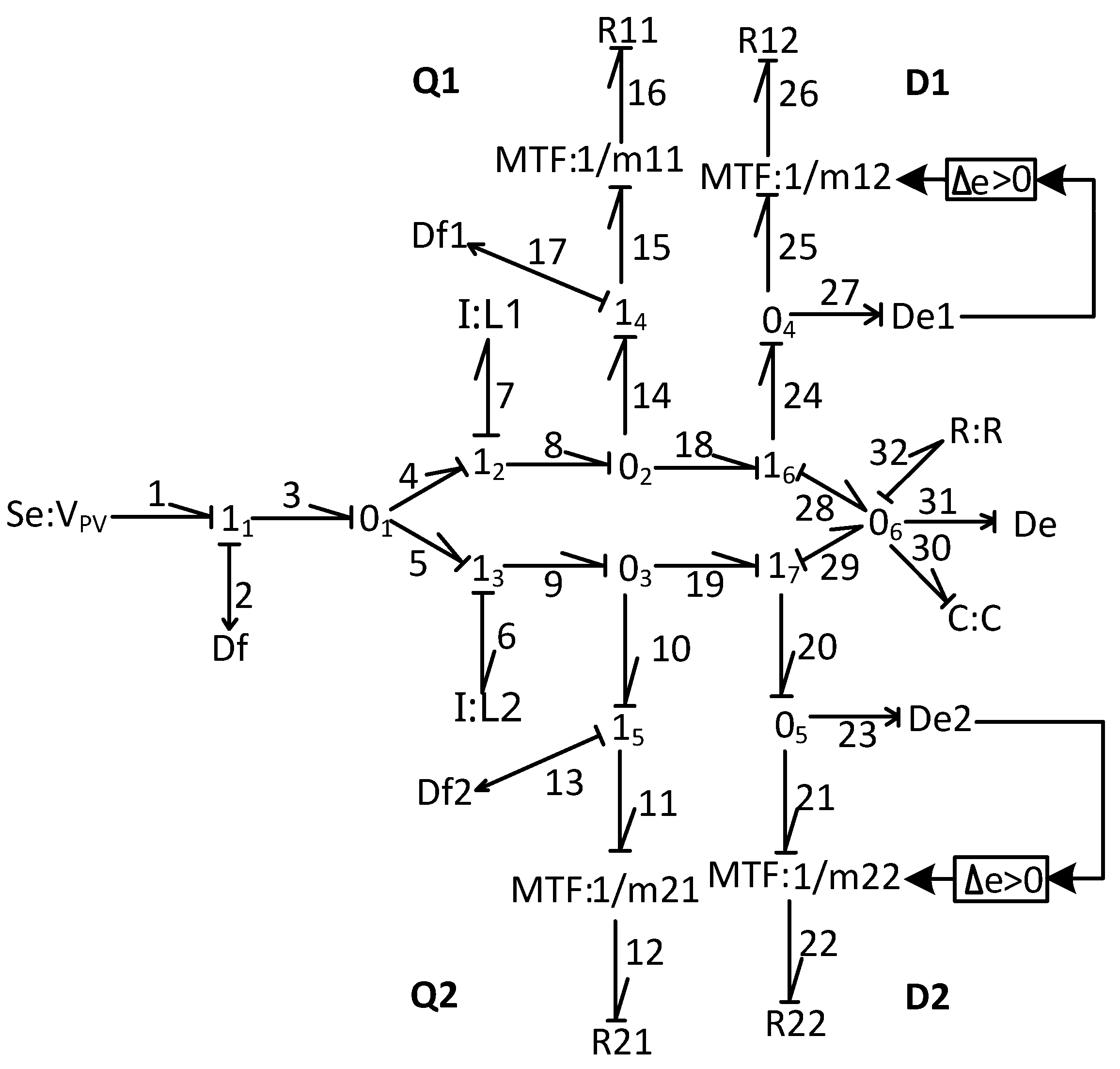
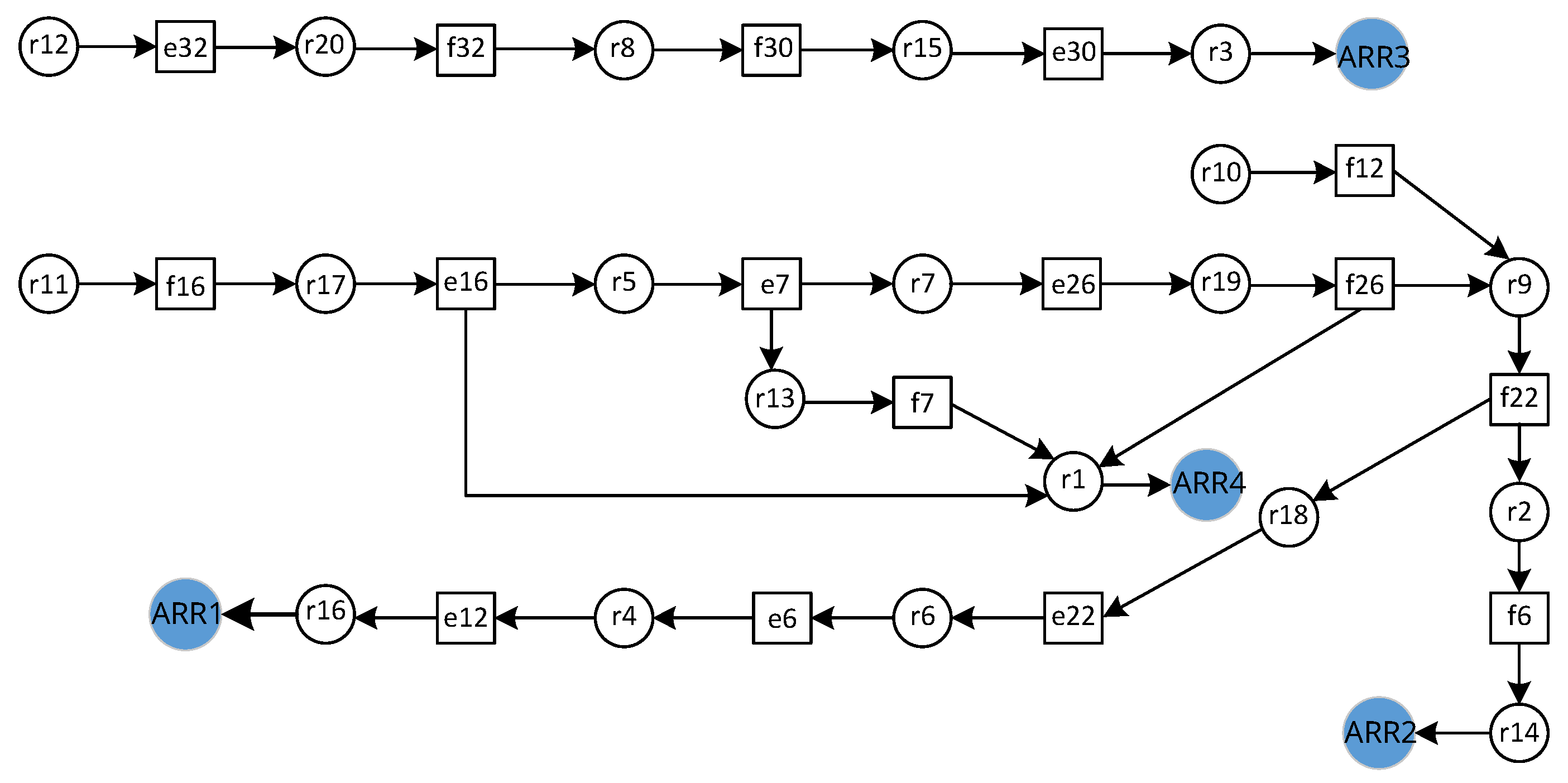
Our research work has two contributions. Firstly, we designed and implemented a cascaded PI-SMC for a two-stage interleaved boost converter (2IBC) that provides passive fault-tolerant control and ensures the continuity of power supply in the event of a stage fault. Secondly, we applied a bond graph-based fault diagnosis method that utilizes the junction structure of the converter’s BG model to deduce analytic redundancy relations through an alternated chain. This method considers discrete component faults such as the inductance and capacitor, and unlike most other articles, it constructs a table of fault signatures and evaluates residuals for the fault detection and identification of the two-stage boost converter.
The key issue with diagnosis is the use of the same ARRs to detect most of the component faults, particularly the capacitor, which should be identified more precisely. Unlike observer analytic methods that typically address only one type of fault, each component in the graphical BG model has a node. As a result, future work can easily combine artificial intelligence with automated power supply supervision to increase the performance of the diagnosis module in the case of unknown signatures.
The paper is structured as follows: Section 2 presents the problem formulation via a case study of the proposed modular power supply and the contribution of the paper. 
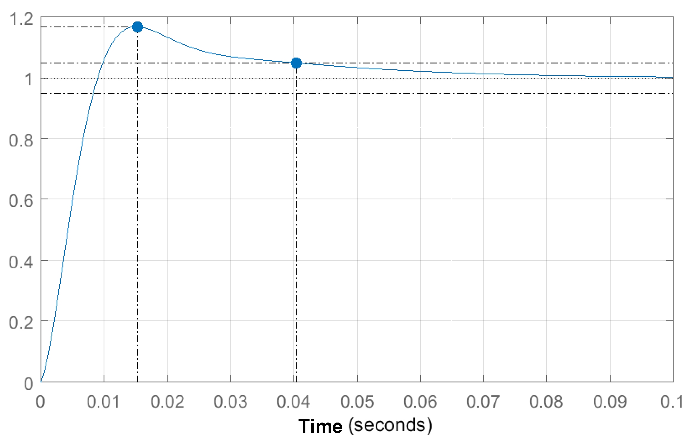
Section 3 explains the selected control strategy for the PV-based system and provides technical guidance for determining the optimal controller parameters. In Section 4, the bond graph formalism is introduced as it applies to power converters and discusses the necessity of hybrid modeling in the same context. Additionally, this section outlines the fault diagnosis approach that is based on the evaluation of residuals to make decisions according to a fault signatures table. Section 5 describes the implementation of the control approach and provides the simulation results of the diagnosis method. In Section 6, the paper concludes with a summary and future directions for research.

2. Problem Formulation and Contribution of the Paper

2.1. Case of Using the Modular Power Supply

Generally, a camping-car with a classic fuel consumption is equipped with two batteries: the primary battery used to start the engine, and an auxiliary battery that typically provides 12 Volts to power on-board equipment such as lighting, water pump, television, and fridge. To produce a 12 VDC power supply from a solar panel, a step-up power converter is required if the panel’s voltage is less than 12 VDC, or a step-down converter if it is higher. However, this power supply is subject to perturbations such as parasitic converter parameters and load variation. Therefore, designing an auxiliary power supply requires a robust control system and a reliable converter structure. The 12 VDC power source is not only needed for starting the engine but also for several applications such as a cigarette lighter, mp3 and mp4 players, etc. While fossil fuel, hybrid, and electric cars have DC power sources with different voltage ranges, 12 VDC is the most common battery voltage value needed, especially in normal cars. A clean 12 VDC auxiliary power source is essential to relieve the primary battery. Photovoltaic power sources provide an alternative to this need. The solar panel can be flexible and lightweight enough to be placed on the roof of small or large camping cars (as shown in Figure 1). Typically, the connection of a solar panel with a 12 VDC auxiliary battery is performed according to the schematic shown in Figure 2. This figure shows the most important equipment that need electricity: fridge, water pump, lighting, and power outlets. This circuit should be protected with a fuse and equipped with relays in the case of intermittent operation.
A low-cost renewable energy source can be designed using discrete components for a boost converter. Boost converters are necessary because PV panels deliver low voltage. It has been demonstrated in [1] that three-stage boost converters are more reliable than conventional ones. However, increasing the number of stages can make implementation difficult, as all stages must be controlled with signals shifted by the same value. This paper presents the design and implementation of an auxiliary 12 VDC power supply based on a 6 VDC solar panel. Due to reliability requirements, the control approach should be robust and fault-tolerant, and the power supply should be supervised by an automated fault detection and identification (FDI) procedure capable of reconfiguring the interleaved boost converter for service continuity. The battery charging process is not within the scope of this study and implementation.

2.2. The Proposed Supervision Scheme and the Fault Tolerance of the Controller

The cascade sliding mode controller is a passive fault-tolerant controller in the proposed supervision scheme of the power supply, as shown in Figure 3. Passive FTC does not require the reconfiguration of the controller when a given set of faults affects the system [13].
The application of SMC for FTC in the real world is varied, and it is frequently used as a controller for power converters. However, when considering SMC as a passive FTC for interleaved converters, the work is still open, and the most frequent use is as an observer. The interleaved power converter involves component redundancy, which facilitates the reconfiguration of the converter. The advantage of a two-stage boost converter is that, in the case of normal operation, the control signals should be shifted with π , and when a stage is faulty, the converter acts as a conventional one with one control signal. This is not the case with a three-stage boost converter when reconfigured to a two-stage one. The shift should be adjusted from 2 π / 3 to π . The diagnosis module is designed based on the ARRs deduced from the BG model in the normal operating mode. The converter collapses when a fault affects the remaining stage. The diagnosis module is designed and simulated with the same control approach implemented in the power supply prototype.

3. The Cascade PI-Sliding Mode Control Applied to the Photovoltaic Power Supply

The proposed prototype is based on renewable energy. It is designed using discrete components for a boost converter to increase the low voltage delivered from a PV panel. In this study, a two-stage converter structure with a duty ratio of 0.5 is chosen, although the same approach can be used for other duty ratio cases. Closed-loop monitoring is necessary, and an efficient control strategy must be implemented to allow for converter reconfiguration in the event of a faulty stage. Subsequently, a diagnosis approach will be developed for a 12 VDC power supply based on a 6 V 30 W PV panel.

3.1. The Renewable Energy Power Supply

The functional diagram of the power supply is illustrated in Figure 4. The choice of an interleaved boost converter is based on the reliability requirements of the DC power source. This paper only discusses the standalone power supply, and the connection with a 12 VDC battery for charging purposes is not addressed.
This prototype can be modular to provide 24 VDC in the case of 6 VDC PV panel (Figure 5a) and 12 VDC PV panel (Figure 5b).

3.2. The Two-Stage Boost Converter Model

The theory behind the construction of an N stage boost converter is presented in [38]. A two-stage interleaved boost converter (2IBC) (Figure 6) requires logic pulse-width- modulated (PWM) control signals u 1 and u 2 for the two transistors with a phase shift of π . Depending on the range of the duty ratio, the operation of the 2IBC converter is divided into three cases: 0.5 < D < 1 , 0 < D < 0.5 , and D = 0.5 .
To further analyze the dynamic behavior of 2IBC, mathematical modeling is required. The state-space averaging technique is commonly used in the modeling of power converters. The paper [38] gives a detailed approach to construct the averaged state space model of a two-stage boost converter. This model is analyzed in CCM with the assumption that the same averaged current was carried in the two stages. The state variables are the inductance’s currents ( i 1 , i 2 ) and output capacitor voltage ( v c ) . The averaged state space model can be written as
x ˙ = A x + b v i n y = c x
with a state vector
x = i 1 i 2 v c
A, b, and c are defined as
A = r L L 0 D L 0 r L L D L D C D C 1 R C , b = 1 L 1 L 0 , c = 0 0 1
where D = 1 D . This model takes into account the parasitic parameter r L of the inductances L 1 = L 2 = L .

3.3. The Application of the PI-SMC Control Approach

The cascade control of boost converters has been identified as an efficient control strategy by experts in the field, as stated in references [11,39]. Therefore, the control scheme for the power supply will be based on this concept. The required performance criteria for the control system are the stability and robustness against parasitic parameters and load perturbations.
Proportional–Integral Cascade Control
In a DC–DC power converter, there is a duality of variables that the controller needs to regulate, including the inductance current and capacitor output voltage. Therefore, the cascade control can be a natural solution, particularly when appropriate sensors are accessible. This approach enables the control system to effectively manage both variables, enhancing the overall system performance.
The cascade control structure of a boost converter is portrayed in Figure 7. The total input current of the converter is i L = i . The same scheme is used for 2IBC with two control signals shifted by π . The transfer functions G 1 and G 2 are defined by
G 1 ( p ) = ı ˜ ( p ) d ˜ ( p ) ; G 2 ( p ) = v ˜ o ( p ) ı ˜ ( p )
These transfer functions are deduced from the averaged state space model (1) by the small signal analysis of the state equations after neglecting the nonlinear second-order terms. The detailed expressions of these functions can be found in [38]. The parasitic parameters are taken into account. C 1 ( s ) and C 2 ( s ) are PI controllers such that
C i ( s ) = K P i + K I i s .
where K P i and K I i are, respectively, the proportional and the integral gains of the controllers. C 1 performs the pursuit of the reference voltage (external loop) and C 2 is dedicated to current regulation (internal loop).
Proportional–Integral Sliding Mode Control
Let us consider the design of the pure sliding mode control on the 2IBC nonlinear model of the form
x ˙ = f ( x ) + g ( x ) u ,
where u R n and x R m are, respectively, the control input vector which is in [ 0 , 1 ] and the averaged system state.
Considering a nonlinear system given by (4), the general design of the control can be performed in two steps: the convergence towards the manifold and then sliding on it to achieve the original. The construction of the manifold is the first step. The general form is proposed by [40]
σ ( x , t ) = ( d d t + λ ) r 1 x ˜ ,
where x ˜ = x x d is the error between the controlled variable and its reference, λ is a positive constant, and r is the relative degree. In the sliding mode control, two conditions have to be satisfied σ ( x ) = 0 and σ ˙ ( x ) = 0 .
The second step is to determine the control law. Generally, the variable structure sliding mode control law is defined by
u = u e q + Δ u .
The first term u e q is continuous; it corresponds to the ideal sliding regime. Δ u is a commutation term in the form of ( k . s g n ( σ ) ) and k is a constant gain. This term lets the equilibrium point close to the sliding manifold.
u e q can be determined by the satisfaction of the invariance conditions
σ ˙ ( x ) = σ x ( f ( x ) + g ( x ) u e q ) | σ = 0 = 0
L f σ ( x ) + [ L g σ ( x ) ] u e q | σ = 0 = 0 ,
where L f σ ( x ) = i = 1 n σ x i f i ( x ) . Then, the expression of u e q will be
u e q ( x ) = L f σ ( x ) L g σ ( x ) | σ = 0 .
In the context of controlling the 2IBC, the sliding manifold can be simply chosen to be
σ ( x ) = λ 1 ( x 2 x 2 d ) + λ 2 ( x 1 x 1 d ) ,
where x 2 d and x 1 d are, respectively, the reference values of the output voltage and the input current and ( λ 1 , λ 2 ) are the parameters of the control only in the case of sliding mode control. In PI-SMC, the reference of the input current is defined by
x 1 d = I L = I L 1 + I L 2 = x 2 d 2 R V i n = V C 2 R V i n .
Due to the fact that boost converters are minimum phase systems, the control of only the output voltage may cause internal instability. When the sliding manifold depends on both current and voltage references, the chattering phenomena will be obvious and the result is poor [11]. The design of the sliding mode control for the current loop in a boost converter does not require the consideration of parasitic parameters. Additionally, it is possible to select f ( x ) and g ( x ) to be equivalent to the expressions of the input-to-output conversion of a conventional boost converter by equalizing the energy stored in the inductors, as described in [1]. To implement the cascaded PI-SMC, the inner PI controller (block C 2 ) is replaced by a sliding mode controller. The sliding manifold will only be based on the inductance current ( σ ( x ) = λ ( x 1 x 1 d ) ).
Since the control signal is discrete in [0,1] and based on (6), the control signal of one converter stage u with λ = 1 will be
u = 0.5 ( 1 s i g n ( σ ) ) .
The stability issue is addressed in [11]. However, the PI-SMC control will give the following performances compared to the pure SMC approach: reducing chattering, greater robustness, fast transient response under load and input voltage variations, and reduced steady state error with guaranteed stability.

4. Fault Diagnosis Using Analytic Redundancy Relations

4.1. Illustrative Example

The bond graph tool was first introduced by [41] in 1961 to primarily represent purely continuous systems. Bond graph modeling uses an analogy to represent all areas of physics, such as electrical, hydraulic, mechanical systems, or grouping several areas mentioned above. It is a structural link graph that facilitates the modeling, analysis, and simulation of physical systems. Analytic redundancy relations (ARRs) are a mature method in BG model-based diagnosis. Let us consider an example of an electrical circuit shown in Figure 8a and its corresponding BG model in derivative causality presented in Figure 8b.
To deduce ARRs, one needs to write the power conservation equations at the level of the two junctions, eliminate all the unknown variables, and write the two analytic redundancy relations ARR1 and ARR2:
r r 1 = D f C d D e d t D e R 2 0 r r 2 = S e L d D f d t D e R 1 D f 0
The first relation is deduced by writing power conservation in the junction 0 (Figure 8) where the effort is equal to the measured voltage D e and the second one is deduced from junction 1 where all nodes have the same flow (current) D f . From the table of fault signatures (which is the same table as Table 1 but without r r 3 ), it will be easy to notice that the faults of D e and D f are detected but cannot be identified because they have the same signature [ d r a 1 , d r a 2 ] = [ 1 , 1 ] . Therefore, a third ARR is needed to identify these faults. Replacing the expression of D f from r r 1 in r r 2 provides this relation
r r 3 = ( 1 + R 1 R 2 ) D e ( L R 2 + R 1 C ) d D e d t L C d 2 D e d t 2 + S e 0
The fault signatures are resumed in Table 1. D and I are, respectively, the detectability of the component fault and its identification. As can be depicted, only the faults of D e and D f could be identified.

4.2. The Bond Graph Model of the Interleaved Power Converter

Several methods have been proposed to incorporate discontinuities in bond graph modeling. Since the early development of bond graphs, it has been necessary to model discontinuities using elements such as switches and valves. In the 1990s, there was a significant interest in hybrid modeling using bond graphs, which was likely driven by the increased computing power of computers. Bond graph switching mechanisms typically work by imposing zero flow or effort on the adjacent structure. For instance, an ideal electric switch (which means no current when closed) or an ideal clutch (which means no torque when disconnected) is consistent with this approach. Furthermore, Soderman et al. [42] used switching trees and ideal elements to formally model mode-switching systems, which involves components with piece-wise continuous behavior, where the system switches between operating modes instead of the on/off behavior.
Mosterman [43] proposed a method for modeling and simulating discontinuities in physical system models by using algebraic constraints. The approach is numerically stable and based on deriving a pseudo Kronecker canonical form. Other researchers [44,45] used modulated transformers (MTFs) to model nonlinear resistance elements. This representation accounts for energy dissipation and does not model ideal switches. In this study, the MTF-R representation was used to model the two-stage interleaved boost converter (2IBC) as it has several advantages: (i) it can be applied to any type of switch; (ii) it provides constant causality; and (iii) the model is physical. The bond graph model of the 2IBC in derivative causality is shown in Figure 9, which includes three current sensors ( D f , D f 1 , and D f 2 ) and a voltage sensor D e . In this model, the diodes do not require an external control signal as they conduct the current when the effort Δ e exceeds a voltage threshold (which is neglected in this case). The control signals of the transistors are the modulated transformers ratios 1 / m 11 ( Q 1 ) and 1 / m 21 ( Q 2 ) .

4.3. Analytic Redundancy Relations Based Diagnosis

The quantitative methods for fault diagnosis are based on physical laws and require a thorough understanding of the system’s structure and numerical parameter values. One advantage of this approach is the simplicity of directly deriving analytic redundancy relations (ARRs) from the bond graph, which is a graphic representation of the physical process.
Two methods can be employed to generate ARRs as identified in [32]: the direct method and the indirect method. The direct method involves recording the connection point relationship between variables (i.e., the causal path) or from the transfer matrix. Indirect methods include substitution and projection. For structural analysis using bond graph models to generate the structure matrix and learn about ARR generation theory, please refer to Appendix A.
The generation of the residuals is generally feasible when the structure of the system is over-constrained and all the unknown variables can be written in terms of the known variables, leading to an analytic redundancy relation. Fault detection based on the bond graph model targets sensor and actuator faults and the structure matrix does not depend on the linearity of the system and is constructed even if its elements can be nonlinear functions of the variables. Matrix M expresses relations of structure and behavior. The rows of the matrix m are independent and the expressed system of equations is over-determined if there is at least one sensor. Given a bond graph model, the corresponding matrix representation leads to a system of equations which does not admit any under-determined subsystem. In other words, the bond graph modeling is consistent and does not generate incomputable variables. The projection method can be programmed symbolically. It is an analytic approach based on solving a linear system of matrix equations. The solution of this system leads to the construction of a projection matrix. This method has the drawback of only being applicable to matrix models resulting from bond graph modeling. We propose the use of the indirect method by substitution. The variables defined in Annex A of the 2IBC are
x ˙ d = [ e 7   e 6   f 30 ] t , Z d = [ f 7   f 6   e 30 ] t , x ˙ i = [   ] , Z i = [   ] D i n = [ e 12   e 16   e 22   e 26   f 32 ] t , D o u t = [ f 12   f 16   f 22   f 26   e 32 ] t Y = [ f 2   f 13   f 17   e 31 ] , U = [ e 1 ] .
The vector V containing all the known and unknown variables will be
V = [ e 7 e 6 f 30 f 12 f 16 f 22 f 26 e 32 e 1 f 7 f 6 e 30 e 12 e 16 e 22 e 26 f 32 f 2 f 13 f 17 e 31 ] t
This representation provides the structure matrix S
S = 0 0 0 0 m 11 0 m 12 0 0 0 0 0 m 21 0 m 21 0 0 0 0 0 0 0 0 0 0 1 0 0 m 21 0 0 0 0 0 0 m 21 m 11 0 0 0 0 0 0 0 m 11 0 m 22 0 0 0 0 0 m 22 m 22 m 12 0 0 0 0 0 0 m 12 m 12 0 0 1 0 0 m 22 m 12 0 0 0 0 0 m 21 m 11 m 22 m 12 0 0 0 0 0 m 21 0 0 0 0 0 0 0 0 0 m 11 0 0 0 0 0 0 0 0 0 0 0 1 0
The matrix M containing the set of information about the bond graph model is illustrated in Figure 10. This representation allows us to construct the alternated chain of Figure 11. The relations r i , where 1 i 20 , are obtained from the equation M . V = 0 . The resolution of this last equation seeks a coupling with respect to the unknown variables. This coupling results in an alternating chain which indicates the sequence of calculation to be followed to express the unknown variables according to the variables to be monitored. The placement of the sensors plays an important role for this resolution. In the case where the generation of an alternating chain is impossible, one can resort to the direct method which always remains applicable (see the illustration example (Section 4.1)) and can be programmed symbolically. For more details on the raised points, the reader can refer to [46]. According to Figure 11, four analytic redundancy relations could be obtained.
The first relation ( r r 1 ):
R 22 m 22 2 R 21 m 21 2 D f 2 + R 22 m 22 2 D f 1 1 R 22 R 12 m 12 2 m 22 2 D e + m 12 2 m 22 2 R 22 R 12 R 11 m 11 2 R 22 m 22 2 D f 2 m 12 2 m 22 2 R 22 R 12 V P V = 0
The second relation ( r r 2 ):
L 2 ( m 21 + m 22 ) s R 22 m 22 D f 2 + L 2 m 21 ( 1 + R 11 R 12 m 12 2 m 11 2 ) s R 22 m 22 D f 1 + R 22 m 22 m 12 2 R 12 R m 22 D e + R 22 m 22 ( 1 m 12 2 m 11 2 R 11 R 12 ) D f 2 R 22 R 12 m 12 2 m 22 + m 22 V P V = 0
The third relation ( r r 3 ):
D f 2 + R 11 m 11 m 12 2 ( 1 + R 12 ) R 12 + 1 D f 1 C s + 1 R + m 12 2 ( 1 + R 12 ) R 12 D e = 0
The fourth relation ( r r 4 ):
L 1 ( 1 + R 11 m 11 2 m 12 2 R 12 ) s + R 11 m 11 2 D f 1 L 1 D e m 12 2 R 12 s V P V = 0
Table 2 represents the fault signatures of the components of the power supply system. The principle is putting “1” when the expression of ARR involves the component.
Several components, such as the transistor Q 1 , diode D 1 , and the solar panel P V , have unidentifiable faults because the fault signatures for these components are not unique. There are various solutions to address this issue, including combining ARRs to deduce new constraints, eliminating components with better reliability, such as sensors, and utilizing artificial intelligence and reliability data to identify the components with the highest likelihood of failure after determining the common signature. It is worth noting that r r i is evaluated with a residual r a i and d r a i denotes the decision about the residual; thus, the procedure would be [1]
d r a i = 1 if | r a i | > δ i 0 otherwise ,
where 1 i 3 and δ i denotes a properly chosen threshold to ensure robustness against false alarms and miss-detection. The practical implementation of residuals detection must follow several steps:
-
Discretization with an appropriate frequency;
-
Digital filtering to reduce false alarms;
-
Numerical limitation to reduce the amplitude of non-desired harmonics. The limit should be higher than the threshold value;
-
The decision must be averaged to an appropriate number of sampling periods to escape the fugitive faults.

5. Simulation and Experimental Results

5.1. The Experimental Prototype

The simulations and the code generation are essentially based on the PSIM tool (https://powersimtech.com/ (accessed on 19 March 2023)). Subsequently, the continuous domain simulation schemes will be translated into the discrete domain for implementation in the digital signal processor (DSP) TI F28335. The control program is generated by the software with the discrete translation of the continuous model by inserting the pulse-width modulation (PWM), the analog-to-digital converter (ADC) DSP modules, and the hardware configuration.
The practical assembly of the power supply is given in Figure 12a. Table 3 and Table 4 display, respectively, the parameters of the 2IBC prototype and the nominal technical characteristics of the solar panel.
The numerical expressions of G 1 ( s ) and G 2 ( s ) are
G 1 ( s ) = ı ˜ ( s ) d ˜ ( s ) = 239.4 s 2 + 17.465 × 10 3 s 22.28 × 10 4 s 3 + 423.3 s 2 + 2.17 × 10 8 s + 1.16 × 10 5 ,
G 2 ( s ) = v ˜ o ( s ) ı ˜ ( s ) = 520.8 × 10 2 s 2 + 26.97 × 10 5 s + 84.63 × 10 5 239.4 s 2 + 17.465 × 10 3 s 22.28 × 10 4 .
The desired step response of the PI–PI cascade control of the 2IBC is given in Figure 13. This curve shows zero static error, an overshoot of 17% at time 0.015 s, and a 5% response time equal to 0.04 s. The parameters of the controllers will be designed according to the performance of this response.
Using the SISOTOOL of MATLAB software, the suitable parameters of the PI controllers can be deduced
K P 1 = 0.0106 K I 1 = 18.12 K P 2 = 0.081 K I 2 = 2.99

5.2. Implementation of the Control Algorithm

Theoretical sliding mode control uses the sign function, but this function performs poorly in practice. Therefore, it is replaced with the saturation function to reduce switching and current ripples. The simulation results of the PI-SMC for the digital model are shown in Figure 14 and Figure 15 after converting the continuous model using Z-transformation and inserting DSP modules. Due to high harmonic components caused by switching frequency, the current signal is filtered with a second-order low-pass filter with a 1 kHz cutoff frequency. The simulation is subject to a 6% load perturbation between 0.25 s and 0.75 s. The converter operates in continuous conduction mode (CCM), and the system accurately tracks 12 VDC. For the nominal operating load, the average values of the simulated output voltage V o and input current of the converter i L over the simulation time of one second are 11.96 V and 0.423 A, respectively.

5.3. Simulation of the Diagnosis Approach

The PSIM software is also utilized for residual simulation using the continuous control approach. The simulation data are then exported to MATLAB for improved curve quality. To filter the residuals, a low-pass filter with a cutoff frequency of 1 kHz is applied. For decision making, the threshold values should be established for all types of failures. However, it is important to note that there is an initial transient state of the residual dependent on the initial conditions, and therefore, the residual values can only be considered after a fixed starting time. Another issue is the sudden change of the residual, which can lead to false alarms and should be disregarded unless it persists over a few sampling periods. These considerations must be verified and validated in subsequent testing.
Healthy System
Assuming that the system is not affected by any fault, the curves of the residuals are illustrated in Figure 16. It can be observed that these residuals are zero if the system is operating normally and a period of 0.015 s is chosen as the starting time of the residual evaluation. This simulation is important to adjust the offset of all the residuals to zero.
Fault of the Current Sensor Df 2
The simulation of a fault affecting the current sensor D f 2 is performed by adding the signal to the sensor output (amplitude = 1 A, startTime = 0.07 s). This gives the residuals of Figure 17. Taking the threshold δ 2 = 0.65 , the detected fault signature would be [1110], which is a fault of sensor D f 2 according to Table 2.
Fault of the Output Capacitor C
A fault of the output capacitor is simulated. It begins at 0.1 s with an abrupt change in the capacitor value (the new value will be half of the nominal 47 μ F). By choosing the threshold δ 3 = 0.47 , the decision d r a 3 of the residual r a 3 will be equal to 1 and we obtain the signature [0010], which is that of the capacitor C (Figure 18). The capacitor fault has a unique fault signature according to Table 2. The identification of the corresponding fault is possible when the residual threshold is chosen correctly. As mentioned in the introduction, this component is the source of the most detected fault in power converters. The proposed approach can identify and detect more than just this fault. This is what will be shown by the sequel. Observer and intelligent methods target one type of fault and it will be hard to design these approaches for an increased number of faults which, in this context, favors the proposed method.
Fault of the Photovoltaic Panel PV
In this case, the fault signature is [1101] (Figure 19) if we consider δ 3 = 4.7 . Otherwise, all the residuals would be active and there will be a faulty identification of the origin of the fault.
Fault of the Transistor Q 1
To simulate this fault, a perturbation signal with an amplitude of 1 and a start time of 0.12 s should be added to the corresponding ratio input of the modulated transformer m 11 . The resulting residual curves are displayed in Figure 20. The signature [1111] can be deduced. According to Table 2, this corresponds to a fault affecting one of the components Q 1 , D 1 , D f 1 , or D e . In this case, to decide the origin of the fault, one should use extra information. This could be, for example, reliability data. m 11 and m 12 are, respectively, associated with transistor Q1 and diode D1, meaning stage one of the 2IBC. These components can be considered with to be of low reliability compared to the sensors D f 1 or D e . Thus, the decision could be a faulty stage of the converter.

5.4. Experimental Results and Discussion

Figure 12b represents the power card of the prototype. The experimental results are resumed in Table 5. These values were measured by a voltmeter at the output of the solar panel and the converter. The error is static, which is calculated as V o 12 12 × 100 .
The experiments conducted in this study did not consider variations in irradiation and temperature. However, random variations were introduced to the input of the converter during testing, which had no impact on the output voltage, as shown in the table. These results confirm the effectiveness of the closed-loop control strategy, which resulted in a static error of only 0.25% even with the input voltage fluctuating at approximately 6 VDC. During the load perturbation test, which involved a 4% increase in charge caused by activating switch S 2 (Figure 12b), the output voltage remained unaffected. Switch S 1 (Figure 12b) was also activated, resulting in the first stage going offline and the circuit becoming equivalent to a conventional boost converter. In this case, the error was of approximately 0.5%, and the same load perturbation had no effect on the output voltage. This experiment demonstrated the hardware redundancy of the power converter, which can overcome the failure of one stage caused by a transistor using the second stage, designed to tolerate the total delivered current. In conclusion, the step-up converter structure was shown to be reliable, and the control scheme’s efficiency was evident under the test conditions.

6. Conclusions and Perspective Work

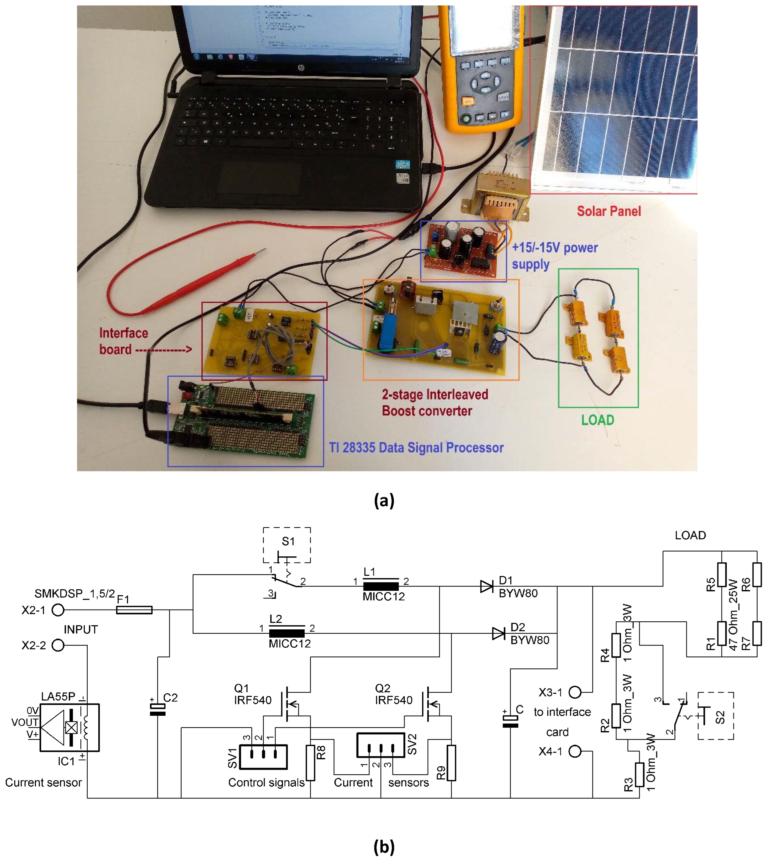
In this paper, a modular PV-based power supply was designed and implemented and an experimental prototype was constructed to validate the proposed control scheme using a real PV panel. The simulations and experimental results demonstrate that the proposed control approach provides good performance. It should be noted that this paper does not cover the variation of irradiation and temperature. Nevertheless, the control scheme can be modified with a maximum power point tracking scheme, and the proposed diagnosis method can still be applied.
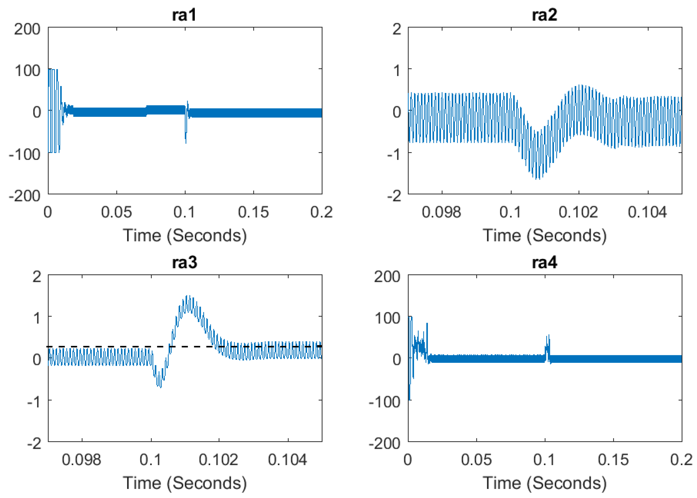
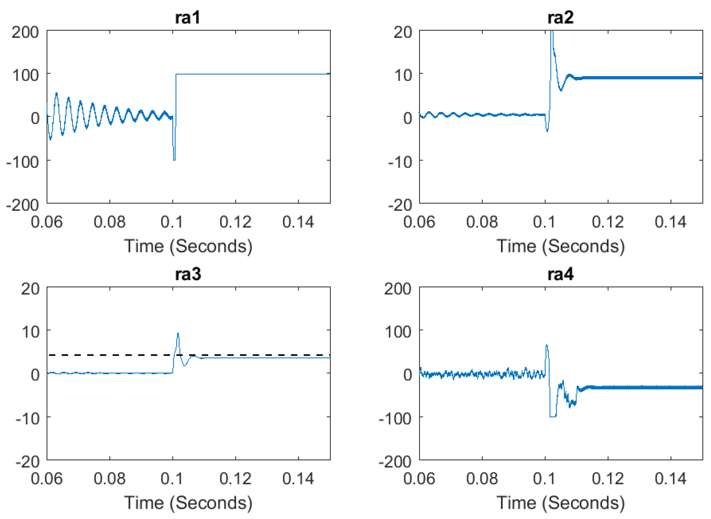
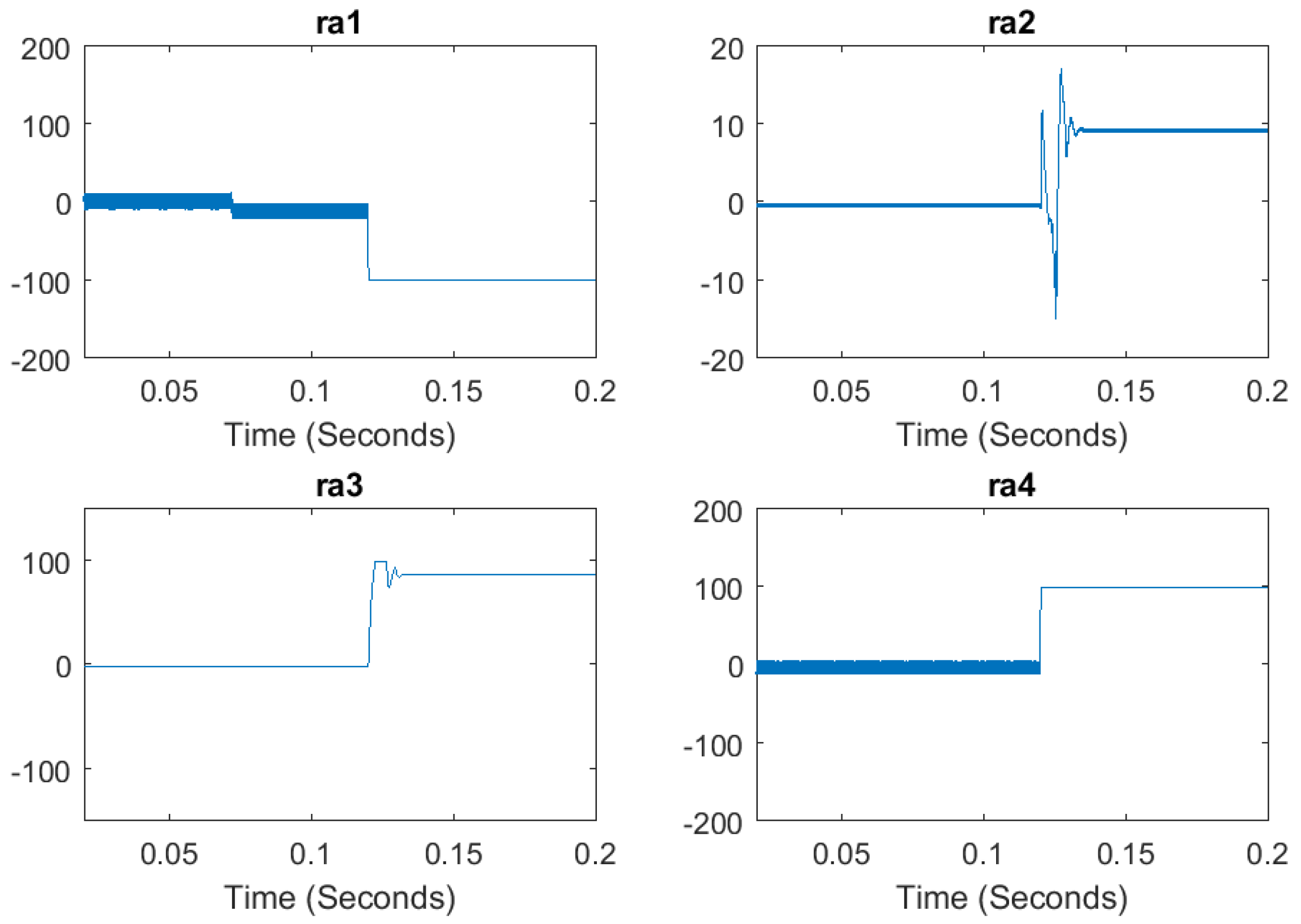
Designing an algorithm for monitoring a physical process can be a challenging task. However, a graphical model that includes all the structural constraints of the process can make this task easier. In this study, a bond graph model-based diagnosis approach was applied to a two-stage DC boost converter. The results of the simulation encourage the implementation of the approach on the real process, which runs in closed loop with a cascaded PI-SMC control algorithm, providing acceptable performance indicators. The switch, sensor, and capacitor faults were successfully simulated and detected. However, the use of an adaptive threshold for the residuals could improve the results for solar panel fault detection.
The most significant work for a BG-based method is performed offline in determining ARRs, which requires an accurate model of the converter. We showed that the proposed approach does not require any learning or database for identifying more than the output capacitor fault. It will be difficult for observer and intelligent methods to treat an increased number of faults.
Identifying faults with identical signatures remains a challenge of this method. Increasing the number of analytic redundancy relations or inserting additional sensors may not always be an effective or feasible solution. To address this issue, resorting to artificial intelligence and additional data on the component reliability is necessary. Future work will focus on establishing the discrete expressions of ARRs, inserting adaptive thresholds, and resolving the detection of identical or unknown fault signatures by incorporating artificial intelligence.
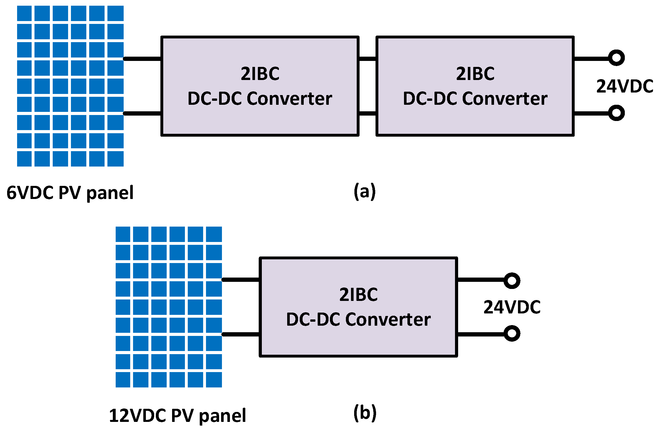
Finally, with a few modifications, this prototype can be adapted to obtain 24 VDC from a 12 VDC solar panel. Additionally, with a two-stage boost converter, it is possible to achieve 24 VDC with a 6 VDC solar panel. The proposed control approach is not limited to specific output voltages and can be applied to other values. If the diagnosis method is correctly implemented, it could provide precise fault detection and enable the real-time monitoring and automated reconfiguration of the power converter.

Author Contributions

Conceptualization, A.Z.; methodology, A.Z. and O.B.; software, A.Z.; validation, O.B. and N.Z.; formal analysis, A.Z., O.B. and N.Z.; investigation, A.Z.; resources, A.Z.; data curation, A.Z.; writing—original draft preparation, A.Z.; writing—review and editing, A.Z. and O.B.; visualization, O.B.; supervision, N.Z. and O.B.; project administration, O.B. and N.Z.; funding acquisition, O.B. All authors have read and agreed to the published version of the manuscript.

Funding

This research was funded by the Tunisian Ministry of Higher Education and Scientific Research.

Institutional Review Board Statement

Not applicable.

Informed Consent Statement

Not applicable.

Data Availability Statement

Not applicable.

Acknowledgments

The authors wish to express their gratitude to the Basque Government through the project EKOHEGAZ II (ELKARTEK 2023), to the Diputación Foral de Álava (DFA) through the project CONAVANTER, and to the UPV/EHU through the project GIU20/063 for supporting this work.

Conflicts of Interest

The authors declare no conflict of interest.

Abbreviations

The following abbreviations are used in this manuscript:
SMCSliding Mode Control
PIProportional–Integral
PVPhotovoltaic
RERenewable Energy
AIArtificial Intelligence
FDFault Diagnostic
FDIFault Detection and Identification
NIBCN-stage Interleaved Boost Converter
2IBC2-stage Interleaved Boost converter
BCBoost Converter
MPPTMaximum Power Point Tracking
CCMContinuous Conduction Mode
BGBond Graph
ARRAnalytic Redundancy Relation
PWMPulse-Width Modulation
DSPDigital Signal Processor
ADCAnalog-to-Digital Converter

Appendix A

The bond graph model can be considered as a junction structure connected to four modules (Figure A1) [47,48]. This structure gives a matrix form showing the junction structure and the different known and unknown variables: storage variables, dissipation variables, sources and sensors. The key vectors associated with this representation are given. The structural bond graph model gives a matrix form showing the junction structure and the different known and unknown variables: storage variables, dissipation variables, sources and sensors.
Figure A1. Structural bond graph modeling.
Actuators 12 00135 g0a1
The key vectors associated with this representation are:
-
X: the state vector (composed of the variables generalized momentum p on elements I and generalized displacement q on elements C) split into the x i and x d vectors associated with the causal components in integral and derivative causalities.
-
X ˙ : the derivative with respect to the time of the state vector (variables e on the I and f on the C).
-
Z: the complement of X (variables f on the I and e on the C) split into Z i and Z d .
-
U: input vector (sources).
-
Y: output vector (sensors).
-
D i n : input of the dissipative module R.
-
D o u t : output of the dissipative module R.
This representation makes it possible to obtain the structure matrix S such that
x ˙ i Z d D i n Y = S 11 S 12 S 13 S 14 S 21 S 22 S 23 S 24 S 31 S 32 S 33 S 34 S 41 S 42 S 43 S 44 Z i x ˙ d D o u t U
S has ( n c + n s ) rows (where n c and n s are respectively the number of components ( I , R or C) and sensors in the system). In the linear case, the following relations can be stated:
D o u t = L . D i n Z i = H ( 1 / s ) . x ˙ i x ˙ d = H ( s ) . Z d
where L , H ( s ) , H ( 1 / s ) are square matrices; s and 1 / s are the derivation and integration operators in relation to time.
Consider the vector V defined by
V = Z i t x ˙ d t D o u t t U t x ˙ i t Z d t D i n t Y t t
This vector contains all the system variables. The matrix M represents the structural relationships and physical constraints of the system
M = S 11 S 12 S 13 S 14 I 1 0 0 0 S 21 S 22 S 23 S 24 0 I 2 0 0 S 31 S 32 S 33 S 34 0 0 I 3 0 S 41 S 42 S 43 S 44 0 0 0 I 4 I 1 0 0 0 H ( 1 / s ) 0 0 0 0 I 2 0 0 0 H ( s ) 0 0 0 0 I 3 0 0 0 L 0
where I 1 , I 2 , I 3 , and I 4 are the identity matrices of suitable dimensions. The matrix M contains enough relations between the variables of the system to constitute a polynomial model: M . V = 0 . This matrix allows us to determine ( 2 n c + n s ) equations and consequently deduce the 2 n c unknown variables of the model [32].

References

  1. Zaidi, A.; Barambones, O.; Charaabi, A.; Zanzouri, N. Fault Tolerant Robust Passivity-Based Control Design for a Proton Exchange Membrane Fuel Cell Power Supply. J. Energy Resour. Technol. 2022, 144, 101304. [Google Scholar] [CrossRef]
  2. Reshma Gopi, R.; Sreejith, S. Converter topologies in photovoltaic applications: A review. Renew. Sustain. Energy Rev. 2018, 94, 1–14. [Google Scholar] [CrossRef]
  3. Sheik Mohammed, S.; Devaraj, D. Simulation of incremental conductance MPPT based two phase interleaved boost converter using MATLAB/simulink. In Proceedings of the IEEE International Conference on Electrical, Computer and Communication Technologies (ICECCT), Coimbatore, India, 5–7 March 2015. [Google Scholar] [CrossRef]
  4. Thounthong, P.; Mungporn, P.; Guilbert, D.; Takorabet, N.; Pierfederici, S.; Nahid-Mobarakeh, B.; Hu, Y.; Bizon, N.; Huangfu, Y.; Kumam, P. Design and control of multiphase interleaved boost converters-based on differential flatness theory for PEM fuel cell multi-stack applications. Int. J. Electr. Power Energy Syst. 2021, 124, 106346. [Google Scholar] [CrossRef]
  5. Olmos-Lopez, A.; Guerrero, G.; Arau, J.; Aguilar, C.; Yris, J.C. Passivity-based control for current sharing in PFC interleaved boost converters. In Proceedings of the Twenty-Sixth Annual IEEE Applied Power Electronics Conference and Exposition (APEC), Fort Worth, TX, USA, 6–11 March 2011; pp. 475–480. [Google Scholar] [CrossRef]
  6. Charaabi, A.; Barambones, O.; Zaidi, A.; Zanzouri, N. A Novel Two Stage Controller for a DC-DC Boost Converter to Harvest Maximum Energy from the PV Power Generation. Actuators 2020, 9, 29. [Google Scholar] [CrossRef] [Green Version]
  7. Arnaoutakis, G.E.; Kocher-Oberlehner, G.; Katsaprakakis, D.A. Criteria-Based Model of Hybrid Photovoltaic–Wind Energy System with Micro-Compressed Air Energy Storage. Mathematics 2023, 11, 391. [Google Scholar] [CrossRef]
  8. Ragusa, M.A.; Tachikawa, A. On some regularity results of minimizers of energy functionals. Aip Conf. Proc. 2014, 1637, 854–863. [Google Scholar]
  9. Ramos-Paja, C.A.; Montoya, O.D.; Grisales-Noreña, L.F. Adaptive Sliding-Mode Controller for Flyback-Based PV Systems Featuring Constant Switching Frequency. Mathematics 2022, 10, 1255. [Google Scholar] [CrossRef]
  10. Al-Wesabi, I.; Fang, Z.; Wei, Z.; Dong, H. Direct Sliding Mode Control for Dynamic Instabilities in DC-Link Voltage of Standalone Photovoltaic Systems with a Small Capacitor. Electronics 2022, 11, 133. [Google Scholar] [CrossRef]
  11. Charaabi, A.; Zaidi, A.; Zanzouri, N. Dual loop control of DC-DC boost converter based cascade sliding mode control. In Proceedings of the International Conference on Green Energy Conversion Systems (GECS), Hammamet, Tunisia, 23–25 March 2017; pp. 1–6. [Google Scholar] [CrossRef]
  12. Frivaldsky, M.; Morgos, J.; Hanko, B.; Prazenica, M. The Study of the Operational Characteristic of Interleaved Boost Converter with Modified Coupled Inductor. Electronics 2019, 8, 1049. [Google Scholar] [CrossRef] [Green Version]
  13. Zenteno-Torres, J.; Cieslak, J.; Dávila, J.; Henry, D. Sliding Mode Control with Application to Fault-Tolerant Control: Assessment and Open Problems. Automation 2021, 2, 1–30. [Google Scholar] [CrossRef]
  14. Liu, Z.; Xu, Z.; Zhang, X. A Novel Real-Time Fast Fault-Tolerance Diagnosis and Fault Adjustment Strategy for m-Phase Interleaved Boost Converter. IEEE Access 2021, 9, 11776–11786. [Google Scholar] [CrossRef]
  15. Abouobaida, H.; Abouelmahjoub, Y.; Marques Cardoso, A.J.; Chikhy, H.; Beid, S.E. Open-Circuit Fault Diagnosis and Fault-Tolerent Control Strategies for Interleaved Boost Converter. In Proceedings of the 2020 IEEE 2nd International Conference on Electronics, Control, Optimization and Computer Science (ICECOCS), Kenitra, Morocco, 2–3 December 2020; pp. 1–6. [Google Scholar] [CrossRef]
  16. Ahmad, M.W.; Gorla, N.B.Y.; Malik, H.; Panda, S.K. A Fault Diagnosis and Postfault Reconfiguration Scheme for Interleaved Boost Converter in PV-Based System. IEEE Trans. Power Electron. 2021, 36, 3769–3780. [Google Scholar] [CrossRef]
  17. Xu, L.; Ma, R.; Zhuo, S.; Xie, R.; Wang, X.; Huangfu, Y. Observer Based Switch Open-Circuit Diagnosis for Interleaved Boost Converter. In Proceedings of the IECON 2020: The 46th Annual Conference of the IEEE Industrial Electronics Society, Singapore, 18–21 October 2020; pp. 5012–5017. [Google Scholar] [CrossRef]
  18. Salman, M.; Dardouri, M.; El Khil, S.K.; Boccaletti, C. Open Switch Fault Diagnosis and Current Sensor Fault Tolerant Control of a DC-DC Interleaved Boost Converter using Generalized Proportional Integral Observer. In Proceedings of the 2021 IEEE 13th International Symposium on Diagnostics for Electrical Machines, Power Electronics and Drives (SDEMPED), Dallas, TX, USA, 22–25 August 2021; pp. 247–253. [Google Scholar] [CrossRef]
  19. Xu, L.; Ma, R.; Zhuo, S.; Xie, R.; Wang, X.; Huangfu, Y. Open-Circuit Switch Fault Diagnosis and Fault- Tolerant Control for Output-Series Interleaved Boost DC–DC Converter. IEEE Trans. Transp. Electrif. 2021, 7, 2054–2066. [Google Scholar] [CrossRef]
  20. He, W.; Shang, Y. Finite-Time Parameter Observer-Based Sliding Mode Control for a DC/DC Boost Converter with Constant Power Loads. Electronics 2022, 11, 819. [Google Scholar] [CrossRef]
  21. Pazouki, E.; De Abreu-Garcia, J.A.; Sozer, Y. Fault tolerant control method for interleaved DC-DC converters under open and short circuit switch faults. In Proceedings of the 2017 IEEE Energy Conversion Congress and Exposition (ECCE), Cincinnati, OH, USA, 1–5 October 2017; pp. 1137–1142. [Google Scholar] [CrossRef]
  22. Guilbert, D.; N’Diaye, A.; Gaillard, A.; Djerdir, A. Fuel Cell Systems Reliability and Availability Enhancement by Developing a Fast and Efficient Power Switch Open-Circuit Fault Detection Algorithm in Interleaved DC/DC Boost Converter Topologies. Int. J. Hydrogen Energy 2016, 41, 15505–15517. [Google Scholar] [CrossRef]
  23. Dieste-Velasco, M.I. Application of a Pattern-Recognition Neural Network for Detecting Analog Electronic Circuit Faults. Mathematics 2021, 9, 3247. [Google Scholar] [CrossRef]
  24. Yang, N.-C.; Ismail, H. Voting-Based Ensemble Learning Algorithm for Fault Detection in Photovoltaic Systems under Different Weather Conditions. Mathematics 2022, 10, 285. [Google Scholar] [CrossRef]
  25. Jamshidpour, E.; Poure, P.; Saadate, S. Common Switch Fault Diagnosis for Two-Stage DC-DC Converters Used in Energy Harvesting Applications. Electronics 2019, 8, 293. [Google Scholar] [CrossRef] [Green Version]
  26. Kumar, G.K.; Elangovan, D. Review on fault-diagnosis and fault-tolerance for DC–DC converters. IET Power Electron. 2020, 13, 1–13. [Google Scholar] [CrossRef]
  27. Sladic, S.; De Santis, M.; Zivic, E.; Giemacki, W. Paradigm Changes in Power Electronics Caused by Emerging Materials. In Proceedings of the International Congress on Advanced Materials Sciences and Engineering (AMSE), Opatija, Croatia, 22–24 July 2022; pp. 1–4. [Google Scholar] [CrossRef]
  28. Zhao, X.; Zhang, X.; Ren, P. Fault Diagnosis and Identification of Power Capacitor Based on Edge Cloud Computing and Deep Learning. Math. Probl. Eng. 2020, 2020, 3120805. [Google Scholar] [CrossRef]
  29. Lu, S.-D.; Sian, H.-W.; Wang, M.-H.; Kuo, C.-C. Fault diagnosis of power capacitors using a convolutional neural network combined with the chaotic synchronisation method and the empirical mode decomposition method. IET Sci. Meas. Technol. 2021, 15, 551–561. [Google Scholar] [CrossRef]
  30. Chaouch, H.; Charfeddine, S.; Ben Aoun, S.; Jerbi, H.; Leiva, V. Multiscale Monitoring Using Machine Learning Methods: New Methodology and an Industrial Application to a Photovoltaic System. Mathematics 2022, 10, 890. [Google Scholar] [CrossRef]
  31. Edstrom, K.; Strömberg, J.E.; Söderman, U.; Top, J. Modelling and simulation of a switched power converter. Simul. Ser. 1997, 29, 195–200. [Google Scholar]
  32. Tagina, M.; Cassar, J.P.; Dauphin-Tanguy, G.; Staroswiecki, M. Bond Graph Models for Direct Generation of Formal Fault Detection Systems. Int. J. Syst. Anal. Model. Simul. (SAMS) 1996, 23, 1–17. [Google Scholar]
  33. Zaidi, A.; Tagina, M.; Ould Bouamama, B. Improvement of Bond Graph Model Based Diagnosis with Bayesian Networks Approach. Int. J. Simul. Syst. Sci. Technol. 2020, 12, 5. [Google Scholar] [CrossRef]
  34. Ould Bouamama, B.; Medjaher, K.; Samantaray, A.K.; Staroswiecki, M. Supervision of an industrial steam generator. Part I: Bond graph modelling. Control. Eng. Pract. 2006, 14, 71–83. [Google Scholar] [CrossRef]
  35. Bouamama, B.O.; Samantaray, A.K.; Medjaher, K.; Staroswiecki, M.; Dauphin-Tanguy, G. Model builder using functional and bond graph tools for FDI design. Control. Eng. Pract. 2005, 13, 875–891. [Google Scholar] [CrossRef]
  36. Yu, M.; Lu, H.; Wang, H.; Xiao, C.; Lan, D. Compound Fault Diagnosis and Sequential Prognosis for Electric Scooter with Uncertainties. Actuators 2020, 9, 128. [Google Scholar] [CrossRef]
  37. Yu, M.; Xiao, C.; Wang, H.; Jiang, W.; Zhu, R. Adaptive Cuckoo Search-Extreme Learning Machine Based Prognosis for Electric Scooter System under Intermittent Fault. Actuators 2021, 10, 283. [Google Scholar] [CrossRef]
  38. Jantharamin, N.; Zhang, L. Analysis of multiphase interleaved converter by using state-space averaging technique. In Proceedings of the 2009 6th International Conference on Electrical Engineering/Electronics, Computer, Telecommunications and Information Technology, Chonburi, Thailand, 6–9 May 2009; pp. 288–291. [Google Scholar] [CrossRef]
  39. Chen, Z.; Gao, W.; Hu, J.; Ye, X. Closed-Loop Analysis and Cascade Control of a Nonminimum Phase Boost Converter. IEEE Trans. Power Electron. 2011, 26, 1237–1252. [Google Scholar] [CrossRef]
  40. Slotine, J.-J.E. Sliding controller design for non-linear systems. Int. J. Control 1948, 40, 421–434. [Google Scholar] [CrossRef]
  41. Paynter, H. Analysis and Design of Engineering Systems; MIT Press: Cambridge, MA, USA, 1961. [Google Scholar]
  42. Soderman, U.; Top, J.; Stromberg, J.E. The Conceptual Side of Mode Switching. In Proceedings of the IEEE Systems Man and Cybernetics Conference—SMC, Le Touquet, France, 17–20 October 1993; pp. 245–250. [Google Scholar]
  43. Mosterman, P.J. Implicit Modeling and Simulation of Discontinuities in Physical System Models. In Proceedings of the 4th International Conference on Automation of Mixed Processes: Hybrid Dynamic Systems, Dortmund, Germany, 18–19 September 2000; pp. 35–40. [Google Scholar]
  44. Back, A.; Guckenheimer, J.; Myers, M. A Dynamical Simulation Facility for Hybrid Systems; Lecture Notes in Computer Science; Springer: Berlin/Heidelberg, Germany, 1993; Volume 736, pp. 255–267. [Google Scholar]
  45. Borutzky, W. Bond graph modelling and simulation of fault scenarios in switched power electronic systems. Inst. Mech. Eng. Part I J. Syst. Control. Eng. 2012, 226, 1381–1393. [Google Scholar] [CrossRef]
  46. Tagina, M. Application de la Modélisation Bond Graph à la Surveillance des Systèmes Complexes. Ph.D. Thesis, Université de Lille, Lille, France, 1995. [Google Scholar]
  47. Borutzky, W. Fault indicators and unique mode-dependent state equations from a fixed-causality diagnostic bond graph of linear models with ideal switches. Inst. Mech. Eng. Part I J. Syst. Control. Eng. 2018, 232, 695–708. [Google Scholar] [CrossRef]
  48. Zaidi, A. Integration of Bayesian Networks and Bond Graphs for Supervision of Dynamic Systems. Ph.D. Thesis, Université de Lille, Lille, France, 2012. [Google Scholar]
Figure 1. Placement of a flexible solar panel on the camping-car roof.
Actuators 12 00135 g001
Figure 2. Connection of PV panel with camping-car installation.
Actuators 12 00135 g002
Figure 3. The supervision scheme including the passive fault tolerant control.
Actuators 12 00135 g003
Figure 4. Functional diagram of the control approach.
Actuators 12 00135 g004
Figure 5. How to provide 24 VDC with the modular converter: (a) with the 6 VDC PV panel; and (b) with the 12 VDC PV panel.
Actuators 12 00135 g005
Figure 6. The two-stage interleaved boost converter topology.
Actuators 12 00135 g006
Figure 7. Cascade PI–PI control of the boost converter.
Actuators 12 00135 g007
Figure 8. Example of an electrical system (a) and its bond graph model (b).
Actuators 12 00135 g008
Figure 9. Bond graph model of the 2IBC in derivative causality.
Actuators 12 00135 g009
Figure 10. The matrix M .
Actuators 12 00135 g010
Figure 11. Alternated chain deduced from M .
Actuators 12 00135 g011
Figure 12. The experimental prototype: (a) a photo of the prototype; and (b) the electronic schematic of the power card.
Actuators 12 00135 g012
Figure 13. The desired output step response of the cascade PI–PI control of the 2IBC.
Actuators 12 00135 g013
Figure 14. Simulation of the input current i L of the converter in the case of 6% load perturbation.
Actuators 12 00135 g014
Figure 15. Simulation of the output voltage V o of the converter in the case of load perturbation.
Actuators 12 00135 g015
Figure 16. Simulation of residuals in the case of a healthy system.
Actuators 12 00135 g016
Figure 17. Simulation of residuals in the case of the sensor Df2 fault.
Actuators 12 00135 g017
Figure 18. Simulation of residuals in the case of an output capacitor C fault.
Actuators 12 00135 g018
Figure 19. Simulation of residuals in the case of a photovoltaic panel fault.
Actuators 12 00135 g019
Figure 20. Simulation of residuals in the case of transistor Q 1 (m11) failure.
Actuators 12 00135 g020
Table 1. Table of electrical system fault signatures.
Se L R 1 R 2 C De Df
r r 1 1110011
r r 2 0001111
r r 3 1111110
D1111111
I0000011
Table 2. Table of fault signatures of the power supply system.
Df Df 1 Df 2 De Q 1 D 1 Q 2 D 2 L 1 L 2 C PV R
r r 1 1111111100010
r r 2 1111111101011
r r 3 0111110000100
r r 4 0101110010010
D1111111111111
I0010000011111
Table 3. The 2IBC technical parameters.
ParameterValue
Input voltage V i n 6 V
Output voltage V o 12 V
Inductance L 1 , L 2 300 mH
Output capacitor C47 μ F
Input capacitor C 2 1000 μ F
Static duty cycle D0.5
Load resistor R50 Ω
Transistor parasitic resistor r O N 0.16 Ω
Inductance parasitic resistor r L 1.1 Ω
Output capacitor parasitic resistor r C 2.1 Ω
Switching frequency F s 10 KHz
Table 4. Technical characteristics of the solar panel.
Maximum power P m a x 30 W
Maximum power voltage V m p 6 V
Maximum power current I m p 5 A
Open-circuit voltage V o c 7.2 V
Short-circuit current I s c 6 A
Size350 × 530 × 17 mm 3
Table 5. Experiments.
Case TestLoad (%) V in (V) V o (V)Error (%)
Open-loop 2IBC1006.8914.5421.16
Closed-loop 2IBC1006.5112.030.25
Closed-loop 2IBC1045.9212.030.25
Closed-loop BC1006.3611.940.5
Closed-loop BC1046.3211.940.5
Disclaimer/Publisher’s Note: The statements, opinions and data contained in all publications are solely those of the individual author(s) and contributor(s) and not of MDPI and/or the editor(s). MDPI and/or the editor(s) disclaim responsibility for any injury to people or property resulting from any ideas, methods, instructions or products referred to in the content.

