Rapid Building Energy Modeling Using Prototype Model and Automatic Model Calibration for Retrofit Analysis with Uncertainty

Abstract

Building performance simulation can be used for retrofit analysis. However, it is time-consuming to create building energy models for existing buildings. This paper presented and implemented a rapid building energy modeling method for existing buildings by using prototype models and automatic model calibration for retrofit analysis with uncertainty. A shopping mall building located in Changsha, China, was selected as a case study to demonstrate the rapid modeling method. First, a toolkit named AutoBPS-Param was developed to generate building energy models with parameterized geometry data. A baseline EnergyPlus model was generated based on the building’s basic information, including vintage, climate zone, total floor area, and percentage of each function type. Next, Monte Carlo sampling was applied to generate 1000 combinations for fourteen parameters. One thousand EnergyPlus models were created by modifying the baseline model with each parameter combination. Moreover, the 1000 simulation results were compared with the measured monthly electricity and natural gas usage data to find 29 calibrated solutions. Finally, the 29 calibrated energy models were used to evaluate the energy-saving potential of three energy conservation measures with uncertainty. The retrofit analysis results indicated that the electrical energy saving percentage of chiller replacement ranged from 1.57% to 13.51%, with an average of 8.27%. The energy-saving rate of lighting system replacement ranged from 1.92% to 11.66%, with an average of 6.43%. The energy-saving rate of window replacement ranges from 0.31% to 1.81%, with an average of 0.55%. The results showed that AutoBPS-Param could rapidly create building energy models for existing buildings and can be used for retrofit analysis after model calibration.

1. Introduction

Climate change has been widely recognized as an important issue. The United States promised to reduce carbon emissions by 50% by 2030 compared to 2005, and the European Union was committed to cutting greenhouse gas emissions by at least 55% by 2030, compared to 1990 levels. Both of them aim to become carbon neutral by 2050 [1]. In 2020, China announced the 3060 climate targets involving reaching the carbon emission peak by 2030 and carbon neutrality by 2060. The building sector is one of the biggest energy consumers and carbon emitters, and it is responsible for a significant portion of greenhouse gas emissions. Globally, CO₂ emissions from the building operation sector increased to 28% of total global energy-related CO₂ emissions in 2020 [2]. Therefore, the mitigation of greenhouse gas (GHG) emissions from buildings was very important.

Building energy simulation is an efficient way to analyze the energy-saving potential of energy conservation measures (ECMs). Ye et al. [3] analyzed the sensitivity of nine different energy-saving measures with EnergyPlus to guide the selection of energy-saving measures in different climate regions. Berardi and Soudian [4] simulated the integration of phase change materials into the envelope with EnergyPlus software to study the energy-saving potential of a passive latent heat energy storage system. Hart et al. [5] used EnergyPlus to simulate the potential impact on the thermal performance of replacing the ordinary glass with triple-thin glass panes and obtained the energy-saving potential in different climatic regions of the United States. Peng et al. [6] used DeST energy simulation software to verify the effectiveness and feasibility of different energy-saving measures in an office building.

The difference between the simulated and measured building energy consumption can range from as high as 250% [7]. In addition, with the increasing use of building energy simulation in the later stages of the building life cycle, the demand for the accuracy of building simulation models has increased significantly [8,9]. Therefore, to ensure the reliability of building simulation models, model calibration has become an important technology in the construction industry [10]. Hong et al. [11] also regarded the calibration of the building model as one of the ten challenges for future building energy conservation.

Calibration approaches can be classified as either manual or automated [12]. Automated calibration approaches involve computerized processes that tune model parameters by maximizing the fit of the model to observations. In contrast, manual calibration approaches rely on iterative, pragmatic intervention by the modeler. Additionally, manual calibration requires a certain level of expertise from the calibration tool, which can be a labor-intensive task. Advanced mathematical and statistical methods enable the automation of the calibration process, which is faster and more efficient than manual calibration [13]. As the complexity of building models increases, manual calibration is gradually being replaced by automated calibration.

Monte Carlo sampling is a class of techniques for randomly sampling a probability distribution, where the distribution of individual parameters will be the same as the inputs [14]. It generates a large number of sample points at random locations to obtain the value that is needed to be calculated. Haarhoff and Mathews [15] presented a simplified Monte Carlo method for finding an approximation of the temperature distribution inside a building; the results showed that relatively accurate results could be obtained with very little data. Chambers et al. [16] used a Monte Carlo model to evaluate the effect of color-changing glass on energy-saving potential. Sørensen et al. [17] used a Monte Carlo simulation to model the energy performance and indoor climate of buildings considering building physical parameters, including properties of facades, walls, and windows, and sift through thousands of combinations of these parameters to find those that meet design criteria. This method could optimize the efficiency of the building design. Zheng et al. [18] proposed a technology-economic-risk decision-making method based on Monte Carlo simulation, which can realize the optimal screening of multiple technology combination strategies. It could also predict regional energy-saving effects and quantitatively analyze energy-saving subsidy policies.

It is a challenging task to manually create a building energy model from scratch. Therefore, it is important to develop a method that can automatically generate building energy models with appropriate accuracy and reduce the time and effort required for model creation while still providing effective analysis. Regarding rapid modeling, part of the research revolves around modeling based on the 3D recognition of buildings [19]. This approach is simpler in principle but is technically demanding and can only model existing buildings. Elisa and Marincioni [20] proposed a method for rapid modeling of end-users connected to the district heating network. The model can be obtained only by obtaining district heating and building volume measurements. For the measures analyzed, the average error was less than 5%.

Due to the inherent uncertainty of the usage factors of building energy consumption, the uncertainty of building energy consumption is inevitable. The more influencing factors, the greater the uncertainty. Prataviera et al. [21] used the proposed procedure to select the most influential input parameters and characterize their uncertainty through positive uncertainty. They conducted measurements on building samples, and the results showed that the average heat load distribution obtained was significantly improved compared to deterministic prototype-based simulations. The overestimation of the peak load of residential buildings decreased from 80% to 25%, and the deviation in energy demand calculations decreased from 18% to 10%. Liu et al. [22] conducted a study on typical high-rise public rental housing buildings in subtropical Hong Kong and found that it was important to consider future climate uncertainty when determining the optimal values of building parameters and selecting building energy renovation plans. Wang et al. [23] investigated the uncertainty of energy consumption caused by actual weather and building operation practices and conducted a simulation-based analysis on a medium-sized office building. The results indicated that the impact of annual weather fluctuations on energy use ranges from −4% to 6%, and good energy use practices have reduced energy use in the entire city by 15–29%. Lu et al. [24] quantified the uncertainty of building energy consumption data based on quantitative uncertainty and Monte Carlo uncertainty propagation methods. Brohus et al. [25] used the method of stochastic differential equation to quantitatively analyze the uncertainty of building energy consumption and conducted two test cases to establish a new prediction method for building energy consumption, which enables designers to include random parameters such as residents’ behavior, operation and maintenance. Chadly et al. [26] conducted an uncertainty analysis of energy storage in a high-energy building in Seattle, and the results showed that batteries are more suitable for the uncertainty of building energy consumption. Kong et al. [27] used Monte Carlo techniques with Latin hypercube sampling to determine the probability distribution of subway spatial peak load, annual average load, and annual energy demand. They also compared it with deterministic methods to determine the rationality of the safety factor of 1.2 commonly used in practical programs.

This study developed a rapid building energy modeling method for existing buildings with monthly measured electricity and natural gas use data. First, a toolkit named AutoBPS-Param (Automated Building Performance Simulation with Parameterization) was developed based on the OpenStudio Software Development Kit (SDK) and EnergyPlus. The toolkit was used to generate the baseline EnergyPlus model based on the building’s basic information, including vintage, climate zone, total floor area, and percentage of each function type. Then, using Monte Carlo sampling, 1000 models and their energy simulation results were output with 14 building parameters in combination. Models that met the calibration criteria were selected by comparing the simulated and measured monthly energy consumption data. The calibrated energy models were used to analyze the energy-saving potential of three ECMs with uncertainty, including windows replacement, chiller replacement, and lighting system replacement.

2. Methods

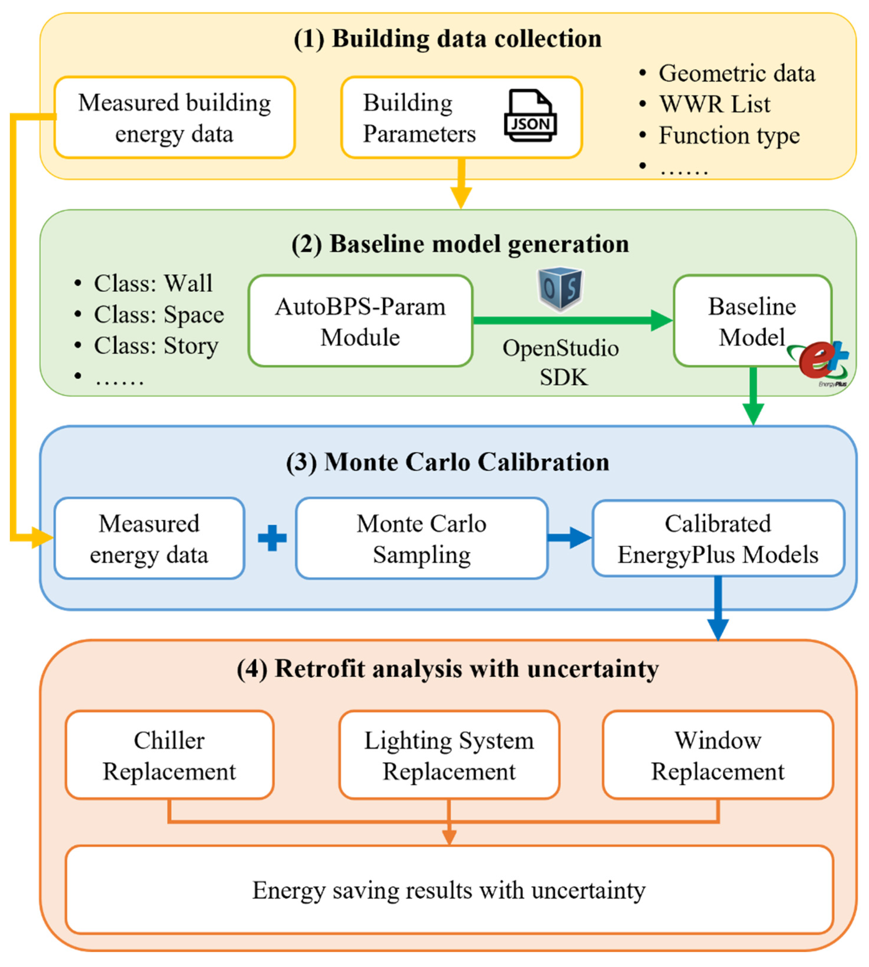
A shopping mall building in Changsha, China, was selected for the case study, where the monthly electricity and natural gas usage data and the detailed layout of each floor were available. Figure 1 shows the overall workflow of this study. First, the basic building information was collected via on-site visits, and the monthly energy consumption data were downloaded from the building management system. Then, a baseline model is generated using the AutoBPS-param based on limited building information. AutoBPS-Param is developed to automatically generate an EnergyPlus model based on basic information, including building type, year built, climate zone, number of stories above and below ground, floor-to-floor height, window-to-wall ratio (WWR) in each direction, width, height, and so on. Users can customize the building geometry while the building systems (envelope, internal zones, heating, ventilation, and air conditioning system) are assigned based on the building type, year built, and climate zone to meet the local and national standards. Moreover, a calibration method based on Monte Carlo sampling was conducted to calibrate the baseline model using measured monthly electricity and natural gas usage data, which can generate multiple calibrated EnergyPlus models. At last, those calibrated EnergyPlus models are used to perform retrofit analysis with uncertainty.

2.1. Basic Information of the Case Study Building

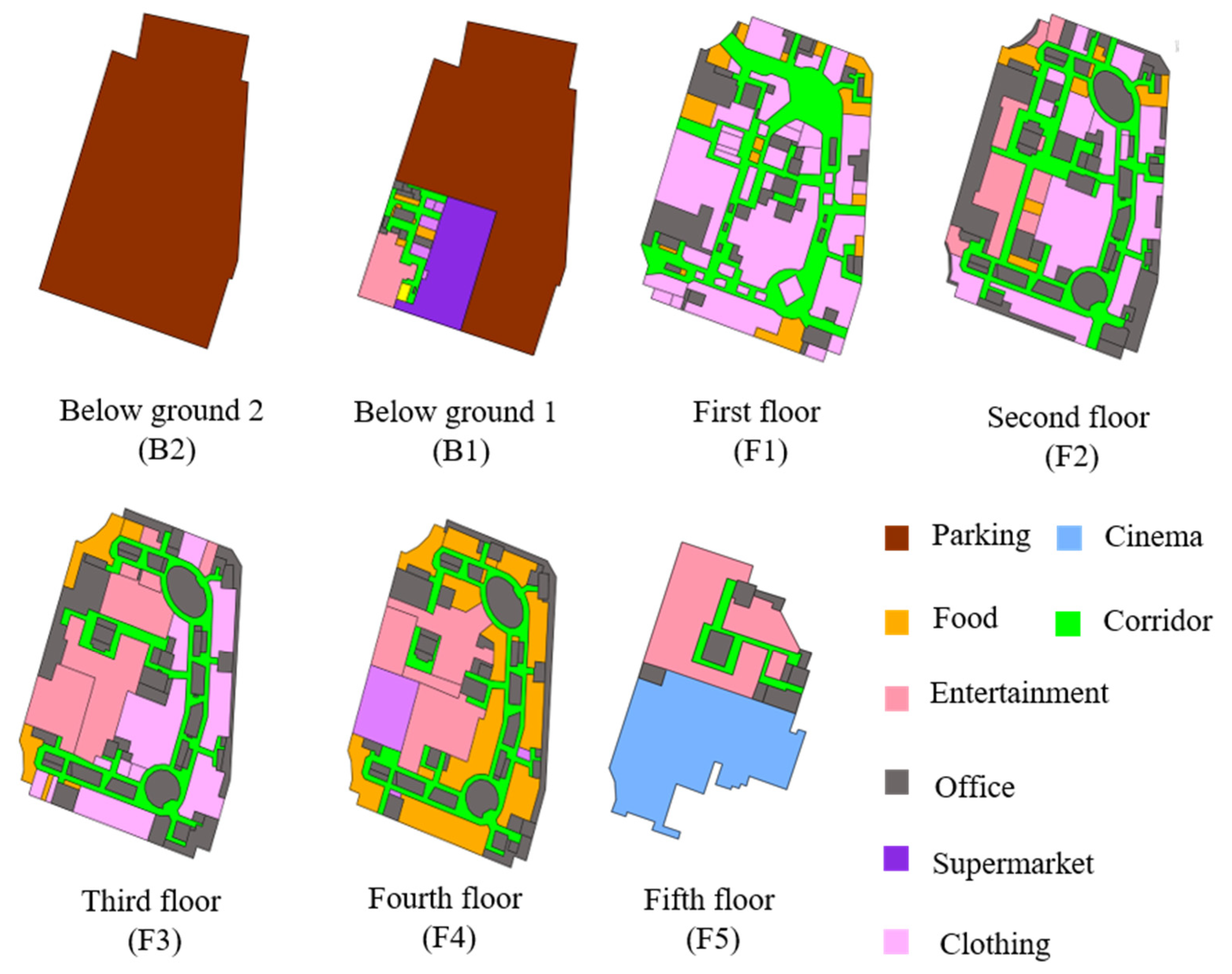
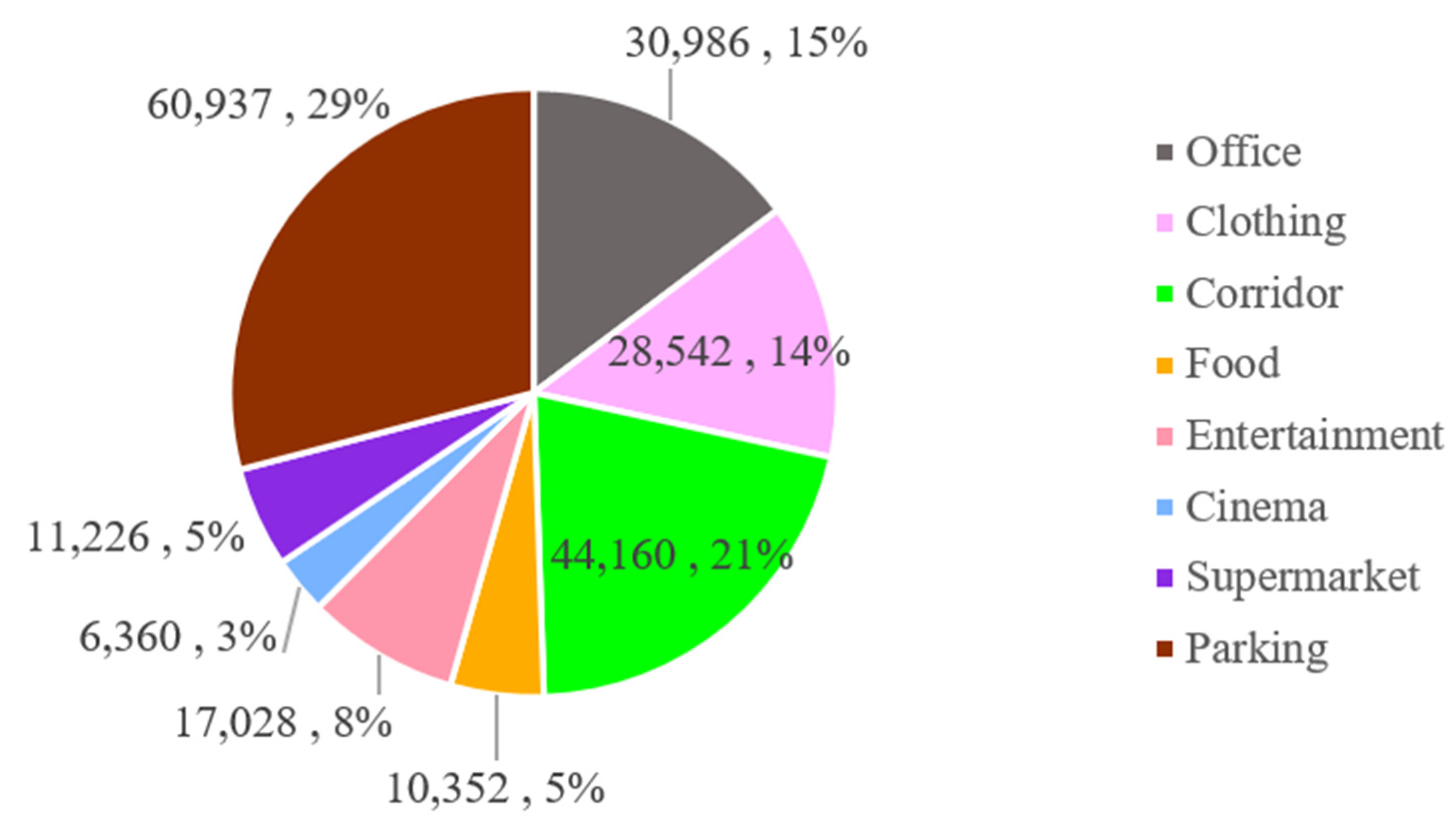
Changsha is located in hot summer and cold winter regions with high humidity throughout the year. The floor-to-floor height of the shopping mall is 4.7 m. The building has windows on the first floors with windows to wall ratio (WWR) of 0.35 on the east, 0.56 on the south, 0.35 on the west, and 0.3 on the north. The building area is 209,591 square meters. Figure 2 shows the floor plans of the building. Through on-site visits and the Baidu map (a web map that is widely used in China), the building is divided into eight functional types for the interior spaces, including parking, food, office, cinema, corridor, clothing, supermarket, and entertainment. The area of each function type is shown in Figure 3.

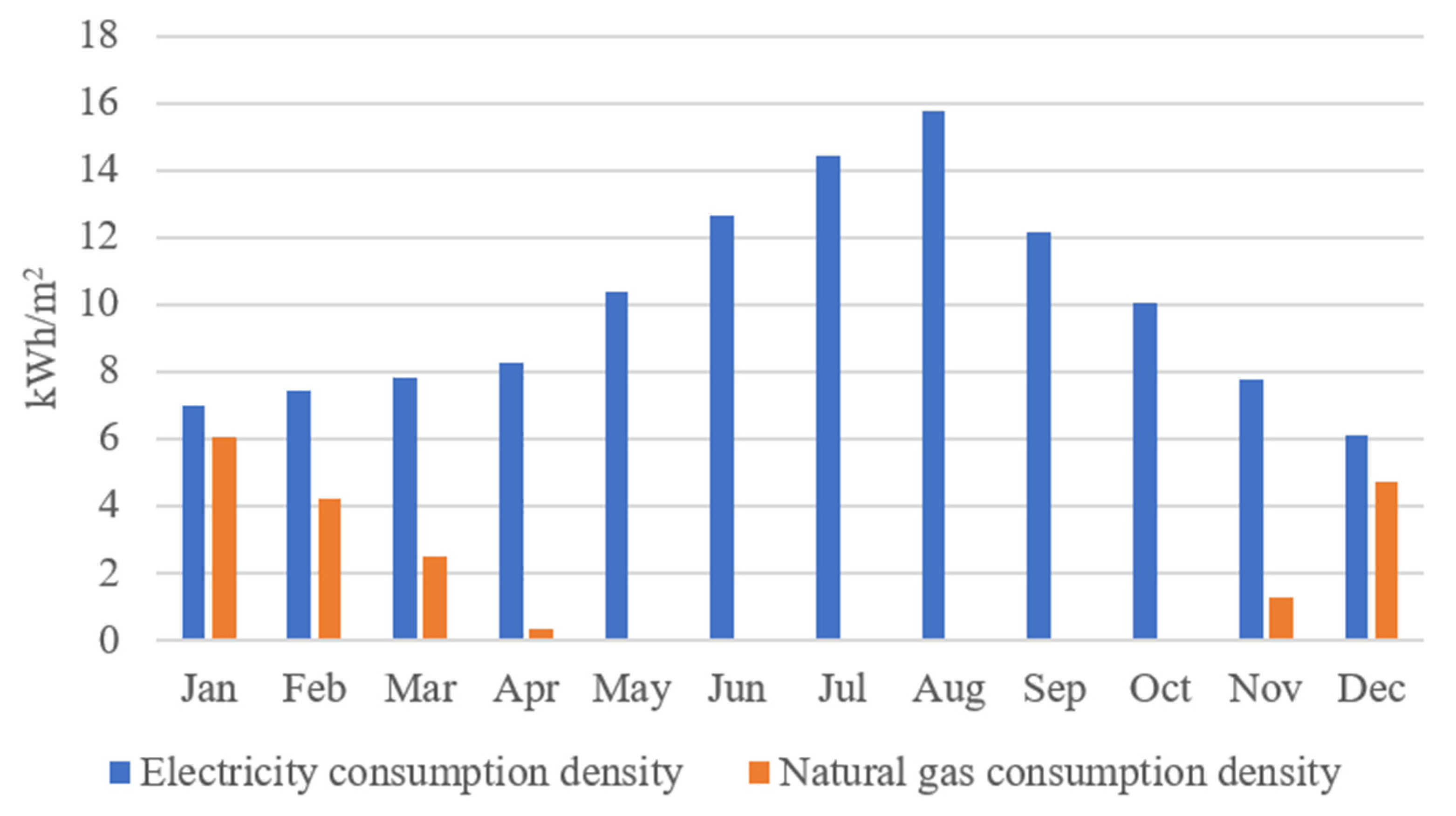
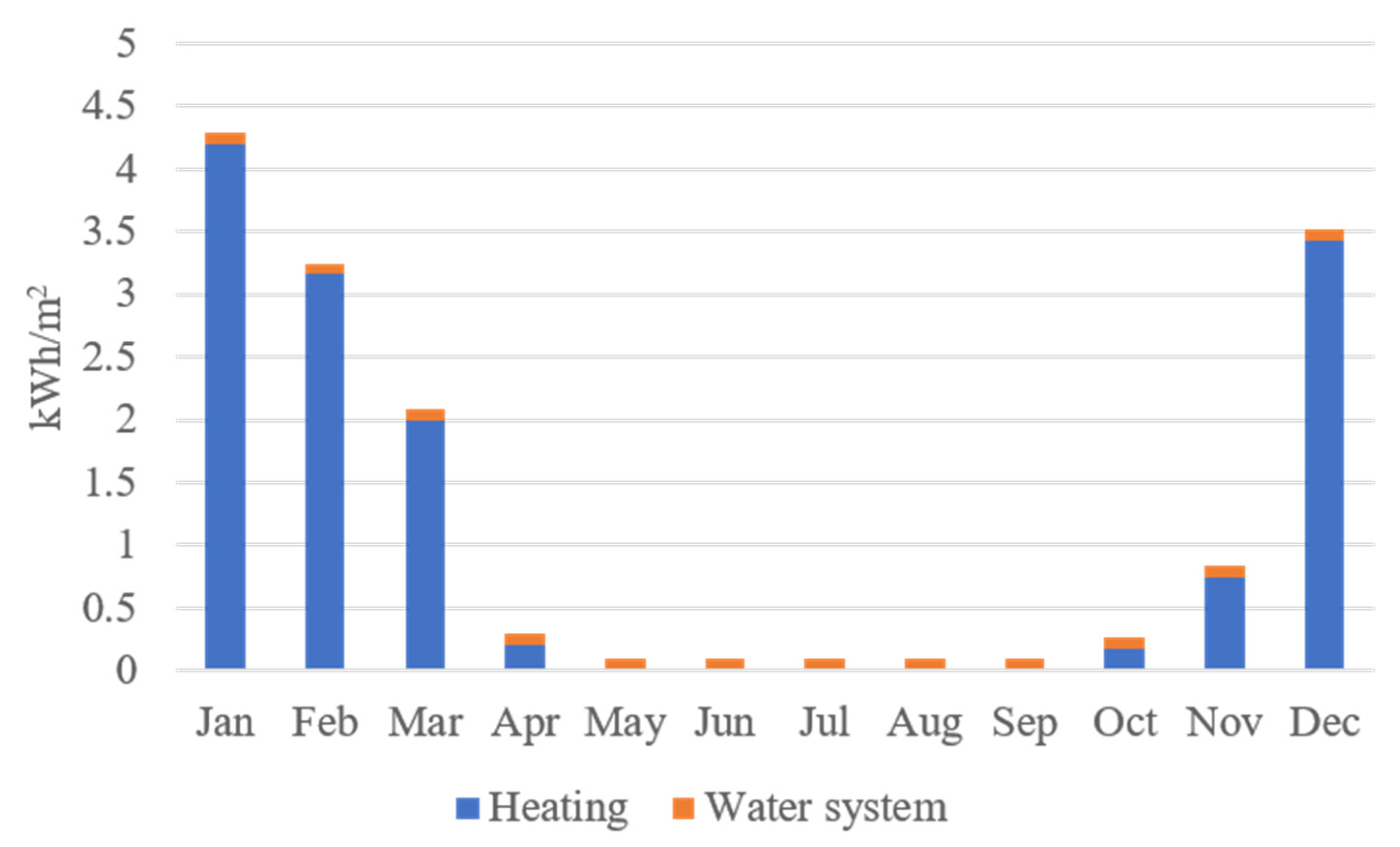
Figure 4 shows the monthly energy usage intensity of electricity and natural gas. The measured annual electricity consumption of the shopping mall is 25.2 GWh, with an electricity consumption intensity of 119.8 kWh/m². The annual natural gas consumption of shopping malls is 14.4 × 10³ GJ, and natural gas usage intensity is 68.6 MJ/m² (19.1 kWh/m²). The electricity consumption intensity of shopping malls shows a parabolic distribution month by month, with the highest electricity consumption density in summer, reaching a peak of 3.0 GWh (15.8 kWh/m²) in July, and the lowest electricity consumption in December, reaching 1.6 GWh (6.1 kWh/m²). The usage of natural gas is opposite to electricity consumption, with the highest usage in winter and spring, reaching a peak of 1.27 GWh (6.0 kWh/m²) in January. Natural gas is not used in summer and autumn.

2.2. Development of AutoBPS-Param

The AutoBPS-Param module was developed to generate the geometric model rapidly, which was based on Automated Building Performance Simulation (AutoBPS). AutoBPS was a Ruby-based platform developed by Hunan University to automate the building energy modeling process from single buildings to urban buildings. Deng et al. [28] developed AutoBPS to generate urban building energy models based on the geographic information system (GIS) dataset in Changsha, then calculated energy demands and analyzed energy retrofit and rooftop photovoltaic (PV) potential. Twenty-two building types and three vintages were identified to represent 59,332 buildings in Changsha [29]. Yang et al. [30] used AutoBPS to establish a bottom-up model to estimate dynamic carbon emission for city-scale buildings in Changsha. Chen et al. [31] developed AutoBPS-BIM to transfer the building information model (BIM) to the building energy model for load calculation and chiller design optimization.

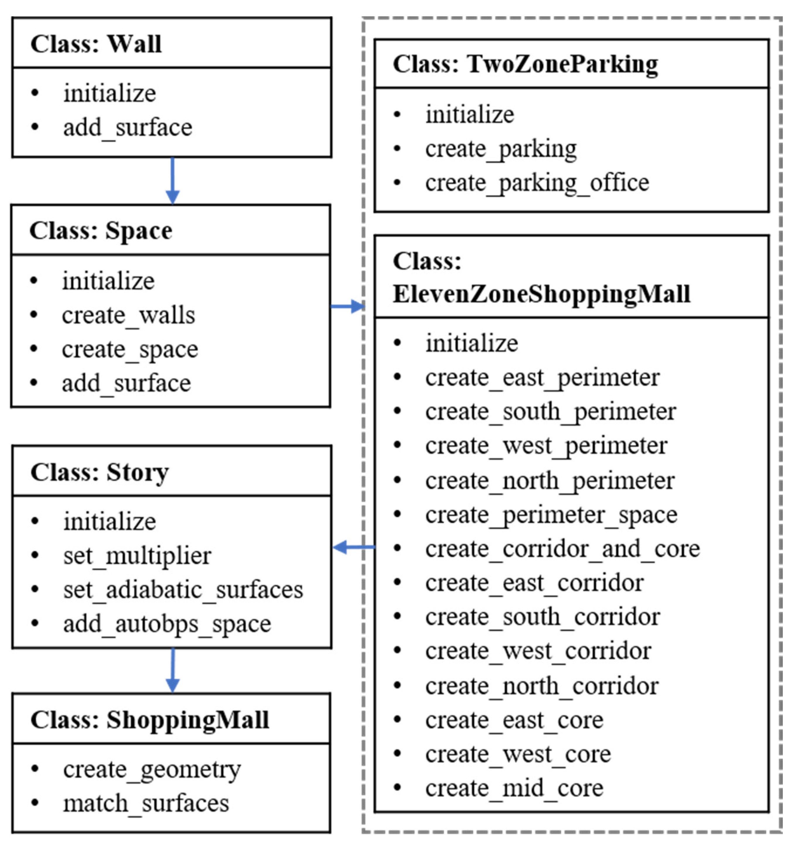
Figure 5 shows the AutoBPS-Param structure for the shopping mall. It relied on OpenStudio Software Development Kit (SDK) and defined some Ruby classes. Some methods were defined under each class. The Wall class was used to create a wall and add windows to the given space. Then, the Space class utilized the Wall class to create a space based on a polygon. The TwoZoneParking class was used to create the underground floor with two thermal zones for the shopping mall. The ElevenZoneShoppingMall class was used to create the standard floor above ground with eleven thermal zones. In addition, the Story class was utilized to set boundary conditions. At last, the ShoppingMall class was applied to create the geometric model by calling other classes.

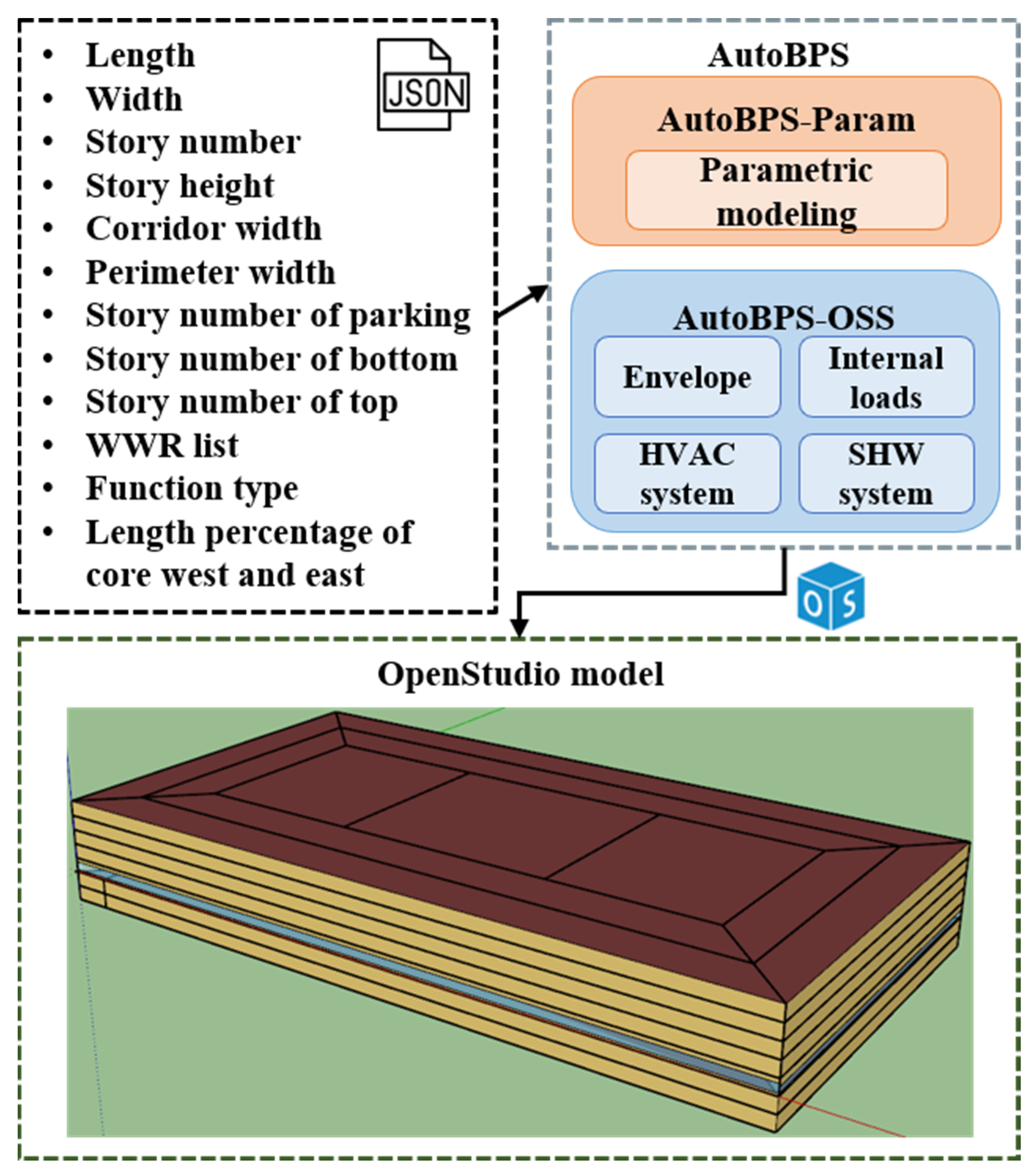
Figure 6 shows the workflow of baseline model generation. To simplify the model, the shape is rectangular with perimeter, corridor, and core areas. Some required geometric parameters are input in JavaScript Object Notation (JSON) format, including length, width, the number of floors, floor height, corridor width, perimeter width, story number of parking/bottom/top, WWR list, space type, length percentage of the west and east core. When the JSON file is ready, the AutoBPS-Param module automatically generates the geometric model. Some non-geometric parameters, such as envelope, internal loads, HVAC system, and service hot water (SHW) system, are assigned to the building through the AutoBPS-OSS module. AutoBPS-OSS is a Ruby-based library based on OpenStudio-Standards (OSS). OSS is developed by the National Renewable Energy Laboratory (NREL) to create American prototype-building models. The Chinese building standards are added to set up the Chinese prototype database. Then, the OpenStudio model is output by two modules.

2.3. Baseline Model Generation

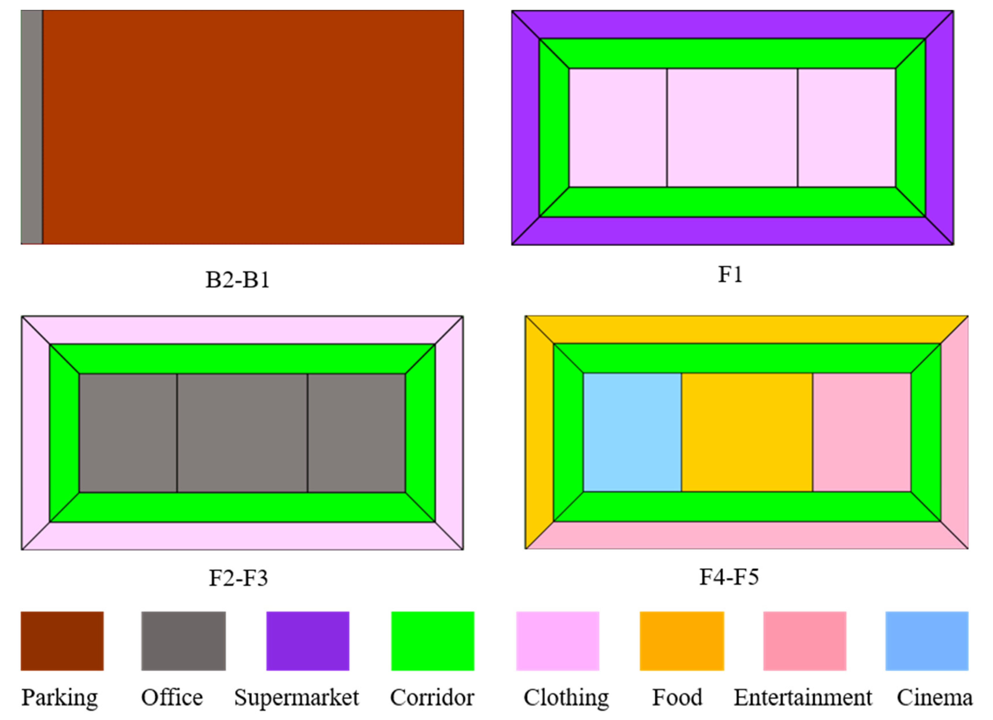
The detailed layout of the shopping mall prototype model is shown in Figure 7. The length and width of the building were 238 m and 126 m. The width of the perimeter and corridor were 15 m and 16 m. There were two parking stories below ground. The spaces in the inner ring were set as the corridor. Other spaces were set up as offices, clothing, food, entertainment, cinemas, and supermarkets while ensuring the basic consistency of floor area as the actual floor area. The second and third floors had the same layout, as did the fourth and fifth floors.

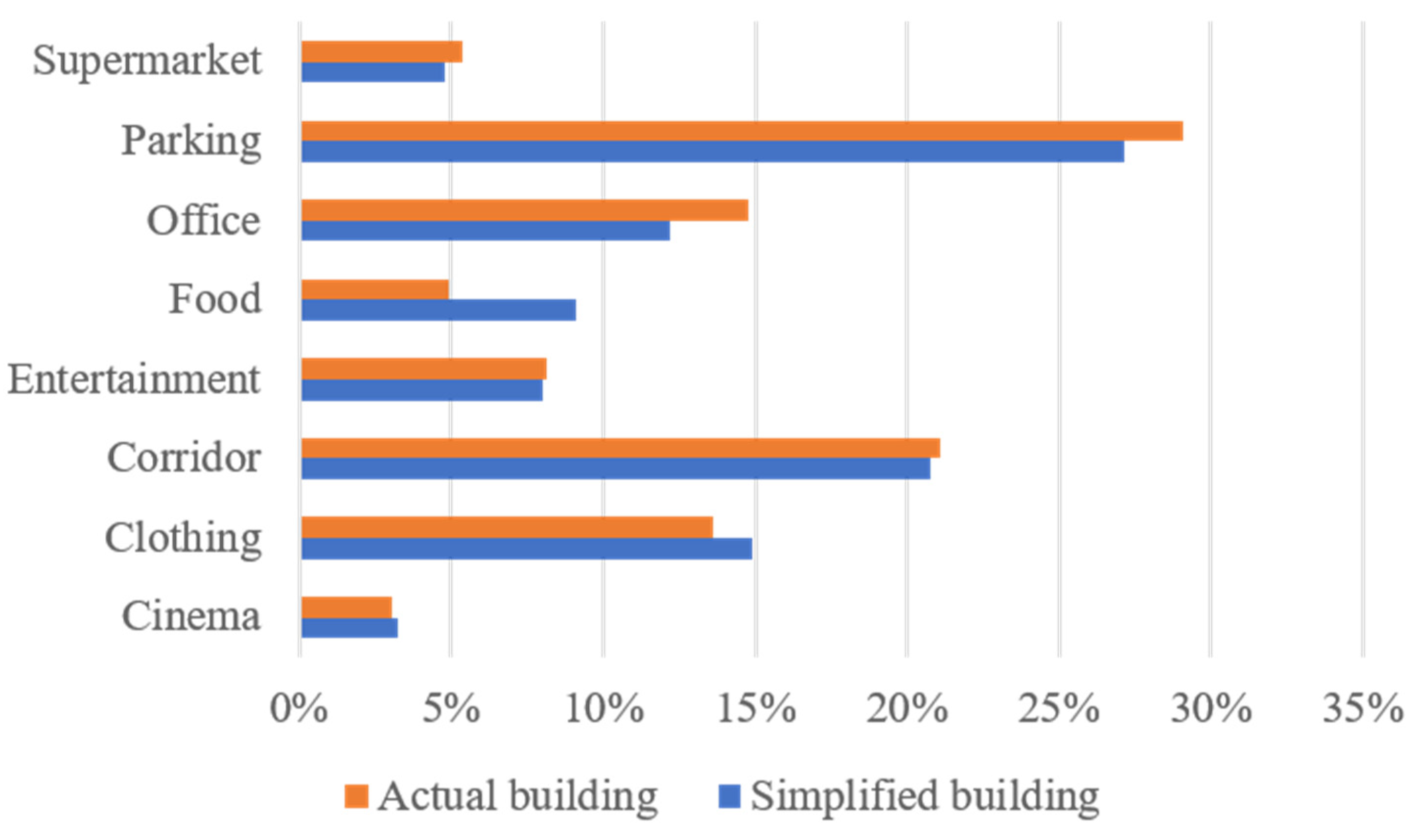
To ensure that the simplified model was consistent with the actual model, the total area of the building and the percentage of the area of each space were compared separately. The actual area of the mall is 209,591 m², and the area of the simplified model is 209,916 m², with a relative error of 0.15%. Figure 8 shows the area ratio of each functional zone before and after simplification. It can be seen that the area share of the actual building and the simplified model were consistent. The relative error was between −0.13% and 4.13%. This also indicated that the simplified model kept the geometric information of the actual building well and had strong reliability.

The building envelope mainly included exterior walls, roofs, and exterior windows.

Table 1. Heat transfer coefficient of the envelope.

		GB50189-2015 [32]	Study Building
Heat transfer coefficient (W/m2·k)	Walls	<0.6	0.58
	Roof	<0.4	0.38
	Window	<2.6	2.5
Window SHGC		0.4	0.4

lists the heat transfer coefficient of external walls, roof, and windows, and the solar heat gain coefficient (SHGC) of windows, which include the values used in this study and the required values in the building energy efficiency design standards of “Energy Efficiency Design Standards for Public Buildings: GB50189-2015” [32].

Since the shopping mall contained different functional areas, the internal load settings for each functional area were different. Through on-site visits and literature reviews, the internal loads of each functional type were determined, including equipment power density, lighting power density, and occupancy density, temperature setpoints in winter and summer.

Table 2. Internal load value table of each thermal zone.

Room Type	Equipment Power Density (W/m2)	Lighting Power Density (W/m2)	Occupancy Density (m2/Person)	Heating Setpoint (°C)	Cooling Setpoint (°C)
Parking	13	5	8	5	37
Supermarket	9	15.5	10	20	25
Corridor	5	9	15	18	28
Food	11	9	10	20	25
Entertainment	9	10	5	20	25
Clothing	13	19	8	20	25
Cinema	11	9	5	20	25
Office	10	10	5	20	25

shows the value of internal gains of each functional type.

The shopping mall’s air conditioning system uses a variable air volume (VAV) system. The building has a central plant with chillers, boilers, and cooling towers. The air conditioning operating hours are from 10:00 to 22:00. The entire air conditioning system consists of four loops, namely the variable air volume system with reheat, the chilled water loop, the condenser water loop, and the hot water loop. The relevant parameter settings of the air conditioning system are referred to in “Building Energy Efficiency Design Guideline: GB50189-2015” [31]. The Coefficient of Performance (COP) of the chiller unit is 5.17, the efficiency of the fan motor is 0.6, and the thermal efficiency of the boiler is 0.8. The peak water flow rate for daily use is 2.3 L/day/person.

2.4. Monte Carlo Sampling

The baseline model was calibrated based on measured monthly electricity and natural gas usage data. Monte Carlo sampling can randomly generate lists of parameter combinations where the distribution of each parameter is the same as the initial settings. Monte Carlo sampling was used to generate representative samples reasonably. The advantages of Monte Carlo sampling are its ability to handle complex problems, such as high-dimensional and nonlinear problems, and the reliability and accuracy of its results. Due to the nature of random sampling, the accuracy of the sampling results increases with the number of samples, making Monte Carlo sampling a very effective statistical method. The steps of applying the Monte Carlo sampling method to building energy consumption calibration are as follows:

Step 1: Define the research problem. The research problem of Monte Carlo sampling calibration lies in the final determination of the parameter values of the model. Since different combinations of parameters may exist to meet the requirements at the same time, the final parameter values are not definite but a series of values that together constitute the parameter distribution.

Step 2: Extract the parameters. The parameters needed for Monte Carlo sampling calibration are the parameters that affect the energy consumption of the building, select the part of the parameters that need to be studied from all the parameters that affect energy consumption, and determine the a priori distribution of the parameters through literature research and so on.

Step 3: Generate random numbers for simulation. For the probability distribution of each parameter, generate a series of random data for experimental simulations. This process generates different combinations of parameters, and EnergyPlus models with different combinations of parameters are run to obtain different energy consumption distributions.

Step 4: Statistical experimental results. The energy consumption results of all simulated models are counted. The discriminant condition needs to be set to discriminate the models that meet the conditions in the model by the fitting accuracy of the measured data and the simulated data. The distribution of parameters is further extracted from the models that meet the accuracy, and the sampling calibration of the sampled models is finally completed.

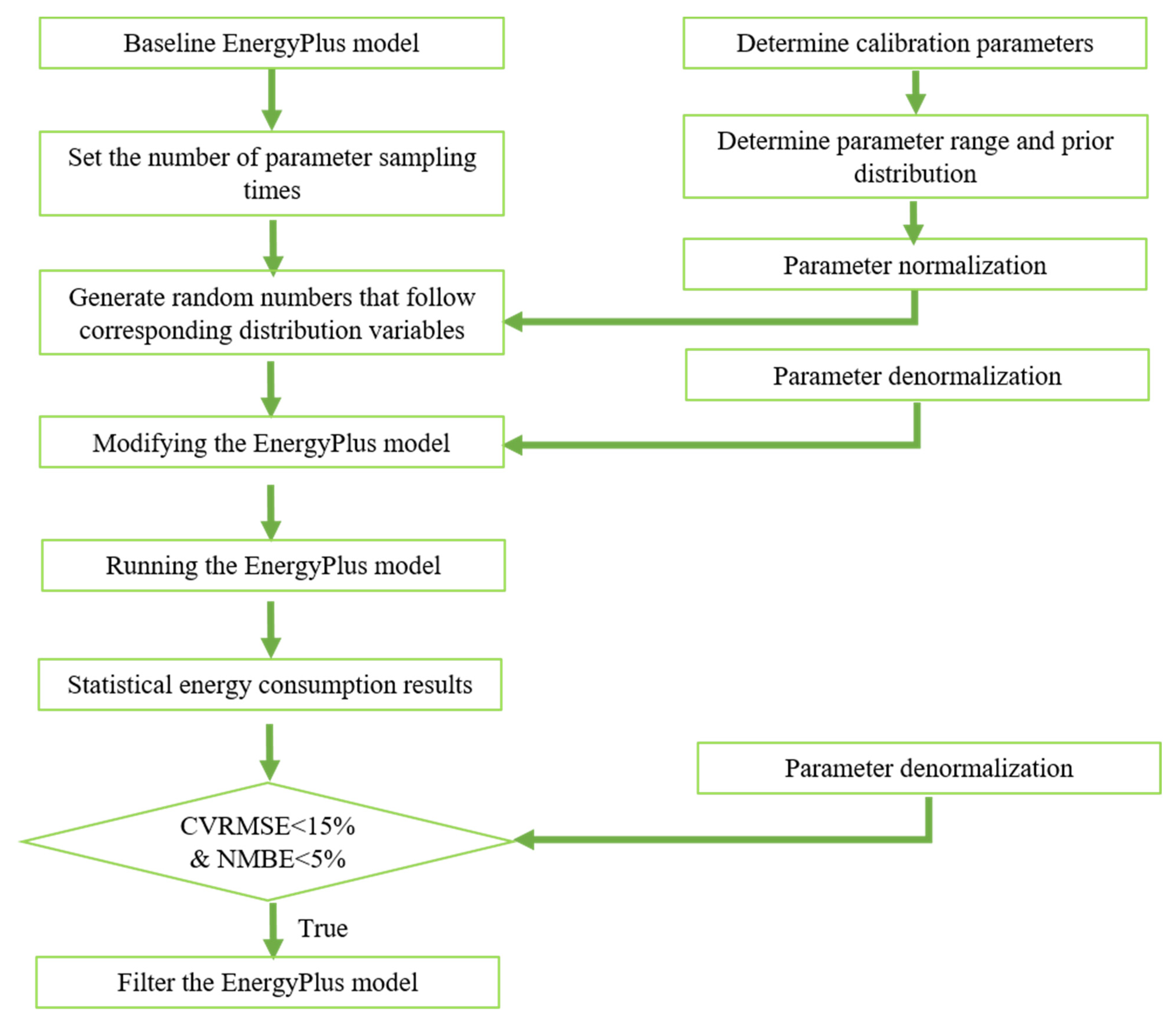
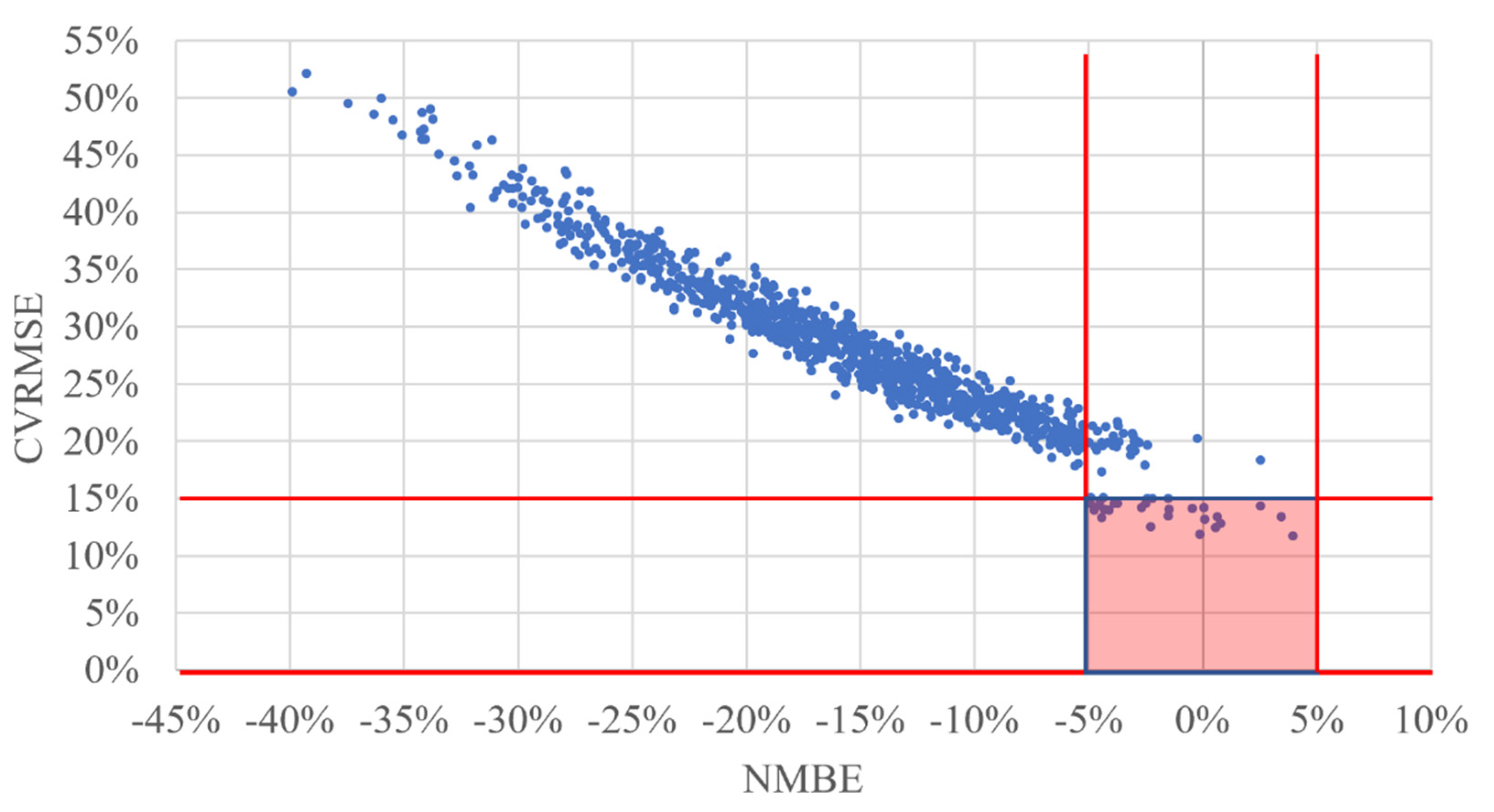
The implementation of the Monte Carlo sampling calibration method is shown in Figure 9. Firstly, based on the established reference model, the parameters that need to be calibrated are determined, and the range and prior distribution of the parameters are established. Next, the number of models to be sampled needs to be set, and the parameters need to be normalized and processed to generate random numbers corresponding to the sampling number. The inverse normalization of the random number is used to modify the actual parameters of the model. The modified EnergyPlus model is run, and the energy consumption results of all sampled models are collected and compared with the measured energy consumption data. Models that meet the calibration criteria based on the normalized mean bias error (NMBE) not exceeding 5% and coefficient of variation of the root mean square error (CVRMSE) not exceeding 15% are selected as the calibrated models. The calibrated models are then used to predict the energy consumption of the building.

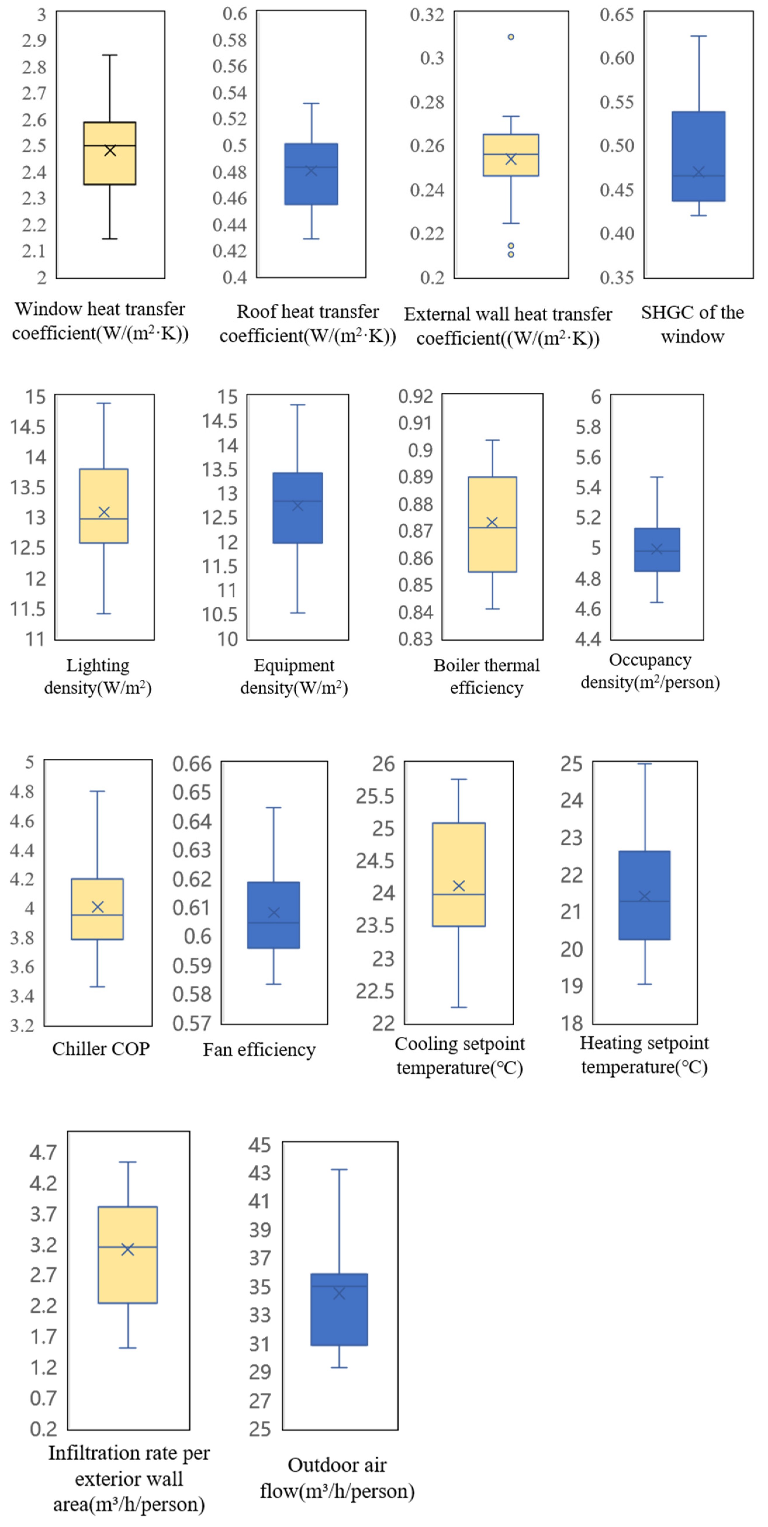
Use Monte Carlo sampling to calibrate the model. The first step is to determine the calibration parameters. This paper finally selected 14 Monte Carlo sampling parameters for the envelope system, internal gain, and air conditioning system, which have a significant impact on building energy consumption. After selecting calibration parameters, it is necessary to set the parameter range and its initial distribution. The range of parameters first refers to the study of Chen et al. [14] and the Chinese national building design standards, including the “GB50189-2005 Energy Efficiency Design Standards for Public Buildings” [33] and “ GB50189-2015 Energy Efficiency Design Standards for Public Buildings” [31]. In addition, the United States Department of Energy prototype strip mall models [34] for ASHRAE 90.1-2016 in climate zone 4A were also studied when determining the range of calibration parameters. In the initial stage of calibration, the maximum value and minimum value of the 14 calibration parameters were given based on the above four references.

Table 3. The range of parameter values in the relevant literature.

Parameter Name	Unit	GB50189-2015	GB50189-2005	ASHER 90.1-2016	Ref [14]
External wall heat transfer coefficient	W/(m2·K)	<0.6	<1	—	—
Roof heat transfer coefficient	W/(m2·K)	<0.4	<0.7	—	—
Window heat transfer coefficient	W/(m2·K)	<4	—	—	1.43~6.98
SHGC of the window	none	—	—	—	0.18~0.82
Occupancy density	m2/person	8	4	20	3~20
Lighting power density	W/m2	10	19	8.5	6.46~27.8
Equipment power density	W/m2	13	13	8.07	8.91~19.1
Infiltration air volume	m3/h/m2	—	—	2.05	1.09~4.08
Fresh air volume	m3/h/person	30	20	28.87	20~50
Fan efficiency	none	<0.65	—	0.61	0.54~0.65
Chiller COP	none	4~6	—	5.33	3.07~5.56
Cooling setpoint	°C	25	—	—	—
Heating setpoint	°C	20	20	—	—
Boiler thermal efficiency	none	0.9	0.89	0.8	0.78~0.93

listed the parameter ranges of some parameters in the four references.

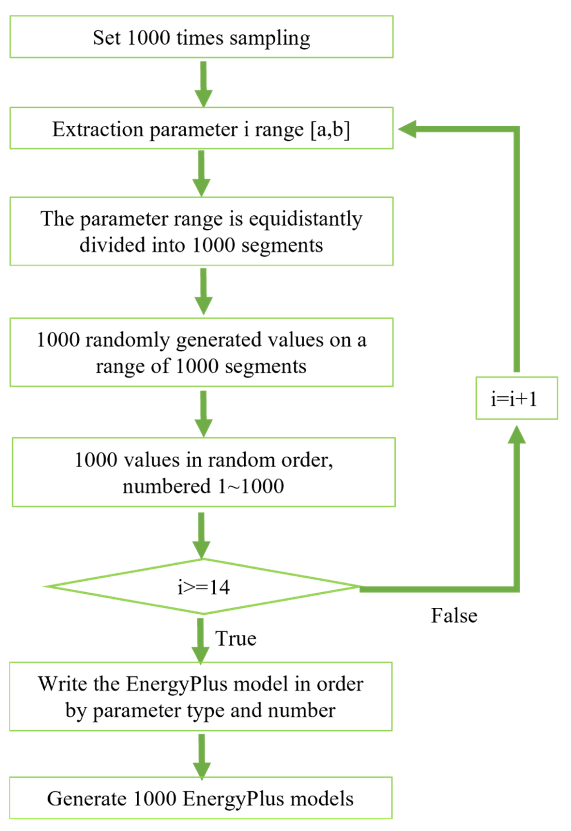
Monte Carlo methods use parameter-based probability distributions for random sampling. A Monte Carlo sampling method based on the Latin hypercube (LHS) can be used to reduce the number of samples while maintaining sampling quality. The LHS samples the sample space by strata, requiring forced sampling from each stratum, thus ensuring full coverage of all samples. To ensure that the values of each parameter are randomly combined, the sample size should be large enough. In this study, a sample size of 1000 is taken. The sampling first divides the range of each parameter into 1000 parts and then randomly selects sample points from each part for random combinations between each parameter while ensuring that the data in each layer can be taken. The specific sampling flow chart is shown in Figure 10.

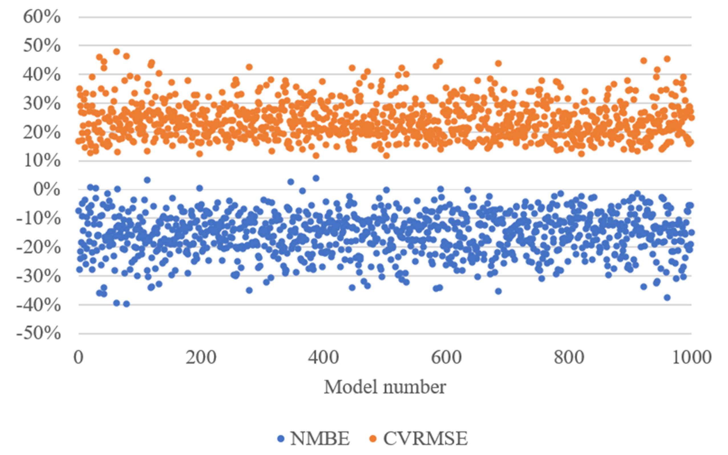
After obtaining 1000 uniformly distributed samples, there will be a certain error between the simulation results and the actual results. Referring to the standard ASHRAE 14 in the United States, the monthly NMBE should not exceed 5%, and the CVRMSE should not exceed 15%.

CVRMSE and NMBE are calculated using Equations (1) and (2):

$$\mathrm{C}\mathrm{V}\mathrm{R}\mathrm{M}\mathrm{S}\mathrm{E}=100\times \frac{{\left[\sum {\left({\mathrm{y}}_{\mathrm{i}}-{\hat{\mathrm{y}}}_{\mathrm{i}}\right)}^2/(\mathrm{n}-1)\right]}^{\frac{1}{2}}}{\overline{\mathrm{y}}}$$

(1)

$$\mathrm{N}\mathrm{M}\mathrm{B}\mathrm{E}=100\times \frac{{\displaystyle \sum \left({\mathrm{y}}_{\mathrm{i}}-{\hat{\mathrm{y}}}_{\mathrm{i}}\right)}}{\left(\mathrm{n}-1\right)\times \mathrm{y}}$$

(2)

where ${\mathrm{y}}_{\mathrm{i}}—$measured data;

$\stackrel{-}{\mathrm{y}}$—mean of measured data;

$\widehat{\mathrm{y}}$—simulated data.

The above formula is only for one-dimensional data for error calculation, and the building energy consumption data are divided into electricity consumption and gas energy consumption. These two parts of energy consumption are different in terms of energy use methods, so they generally cannot be synthesized in one dimension by simple summation. Refer to the formula in Energy Savings Analysis: ANSI/ASHRAE/IES Standard 90.1-2016 for source energy consumption [35]. Source energy is calculated using Equation (3):

Source energy (GJ) = 3.167 × Electricity (GJ) + 1.084 × Natural Gas (GJ)

(3)

Here source energy is defined as an indicator of building energy consumption, including electricity for HVAC (chillers, refrigeration, fans, and pumps), indoor lighting, indoor equipment, and natural gas for heating. The definition of source energy can be used to more easily quantify the error between measured and simulated energy consumption in buildings.

2.5. Retrofit Analysis with Uncertainty

Energy efficiency improvement of buildings can improve energy utilization efficiency by adopting various energy-saving technologies and management measures to reduce building energy consumption. Therefore, energy efficiency improvement of buildings plays an important role in promoting energy saving, environmental protection, economic development, and social progress. There are several ways to perform energy efficiency improvement of buildings, including (1) adding insulation to the building, reducing the heat transfer coefficient of the envelope structure, and reducing the heat loss of the building; specific measures include adding external and internal insulation to the building envelope and roof, replacing to double-layered vacuum insulation glass, etc. (2) Connecting the building to renewable energy resources, such as solar energy and wind energy, for power generation and heating. Specific measures include adding the photovoltaic system to the roof. (3) Using more efficient energy-saving lights and appliances to reduce building energy consumption. With the widespread use of computer technology and various sensors, implementing energy monitoring and safety management is also a new direction for energy efficiency improvement. Through systematic analysis of building energy consumption, problems related to energy consumption can be found and solved more specifically.

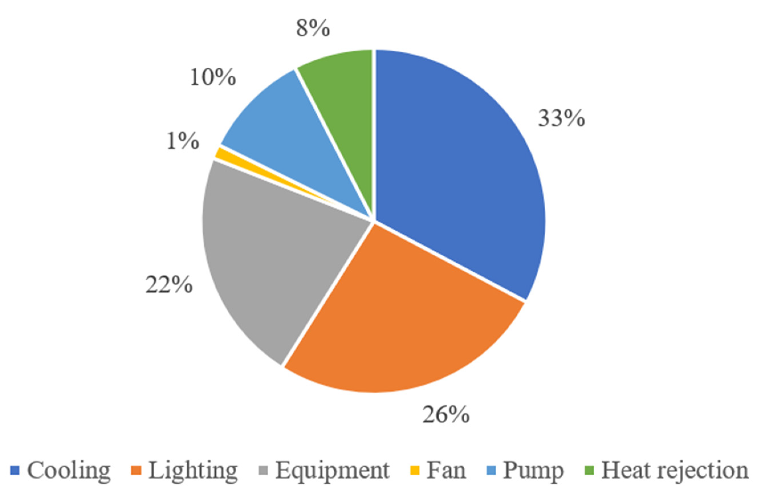
After model calibration, the calibrated energy models can be used for retrofit analysis to evaluate energy saving potential of ECMs. When performing energy efficiency improvement of buildings, it is necessary to analyze the energy consumption of the building. For the convenience of research, the baseline energy model was selected as the research object to analyze its energy consumption situation. The simulated electricity consumption result of the baseline energy model is shown in Figure 11. The two highest percentages of energy consumption are cooling energy consumption for chillers (33%) and lighting energy consumption (26%).

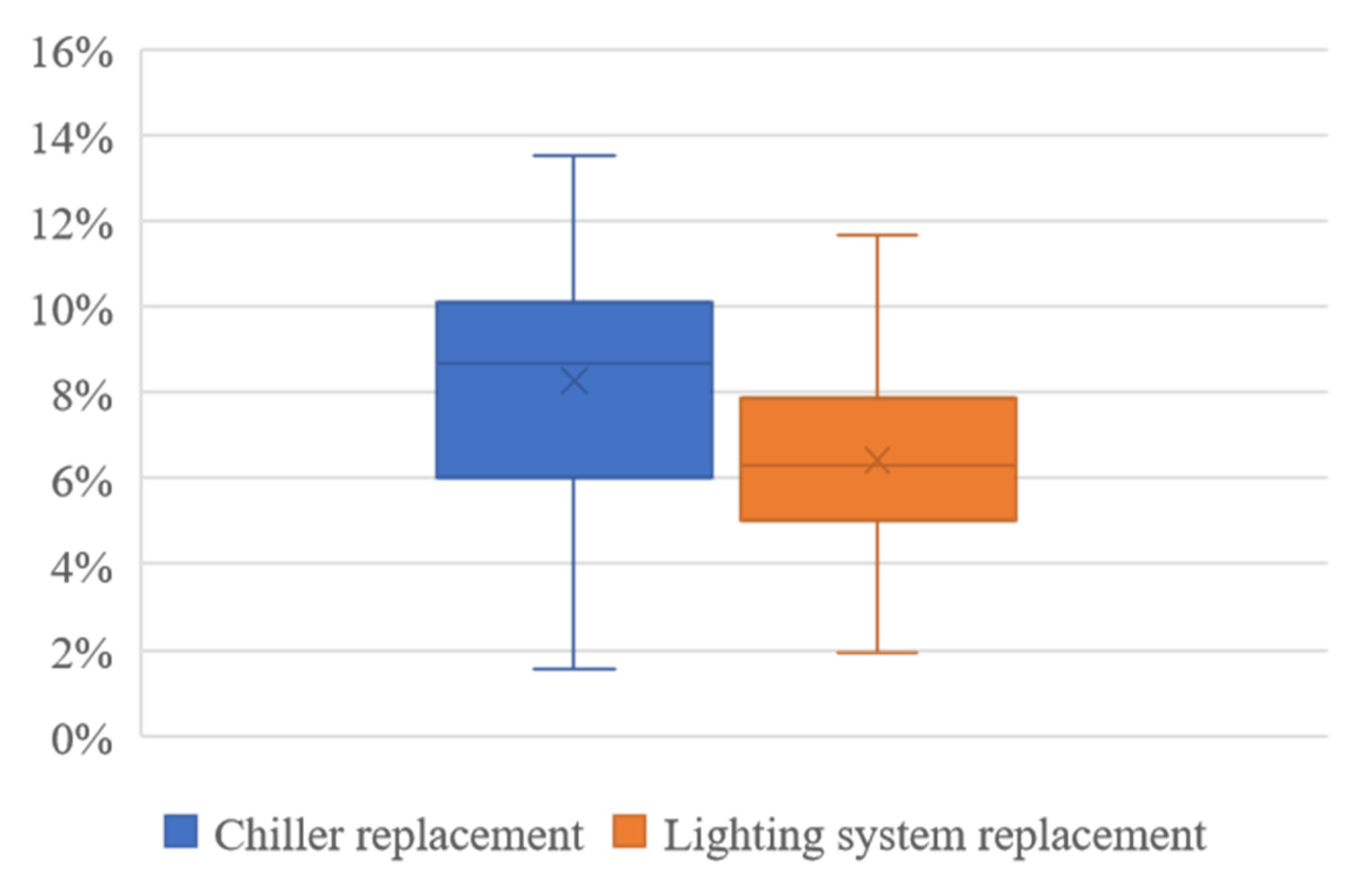
Many measures can be taken to reduce cooling energy consumption, such as using efficient cooling systems, protecting the normal operation of the cooling system, maintaining good insulation of the cooled space or object, and reducing the time of cooling system used. Reducing cooling energy consumption can not only reduce energy costs but also reduce the negative impact on the environment. The main factor affecting the cooling energy consumption is the COP of the chillers. Therefore, strategy A to improve energy efficiency is to replace the chillers.

Lighting energy consumption is determined by multiple factors, including the type of bulb, power, and usage time, as well as the efficiency of the lamp. In general, lighting is one of the major uses of electricity in ordinary homes and commercial buildings, and reducing lighting energy consumption is an important means to improve energy efficiency and reduce energy costs. The size of lighting energy consumption is mainly determined by the lighting system; therefore, strategy B to improve energy efficiency is to replace the lighting system.

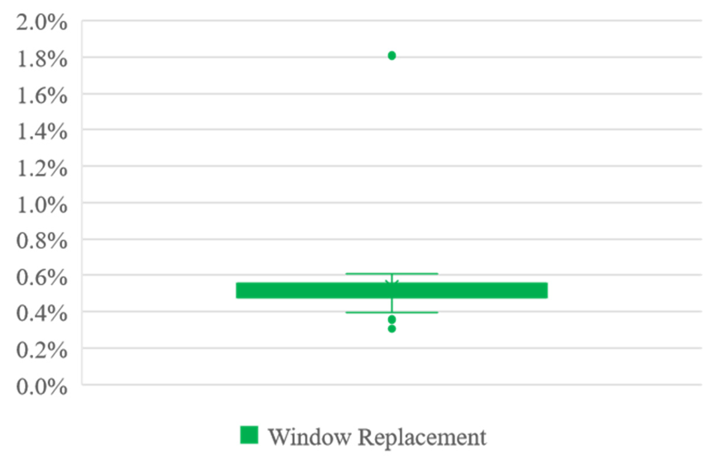
Roberti et al. [36] conducted an energy retrofit analysis of an old building in northern Italy, specifically on the building envelope, including the insulation of the exterior walls and roof and the replacement of windows. The study provides a complete picture of the energy-saving potential of the building envelope, especially concerning window replacement. This paper draws on that study for the replacement of windows in shopping malls. Therefore, strategy C to improve energy efficiency is to replace windows.

There is uncertainty when performing retrofit analysis of ECMs. There are two main sources of uncertainty in energy efficiency retrofitting consisting of two aspects: First, the type of building parameters and their range, and since this paper mainly studies the relationship between building-related parameters and energy consumption, the uncertainty of building-related parameters leads to the uncertainty of energy consumption. The second is the calibration process and its sampling quantity. Since this paper uses the measured energy consumption to calibrate the energy consumption of the sampled models, the building models that meet the calibration criteria are selected, and these models together form the calibrated models.

The establishment of the energy efficiency retrofit model in this study is completed by the modification of relevant parameters in the calibrated shopping mall EnergyPlus models. The energy savings rate indicates the reduction in energy consumption per unit area after the energy efficiency retrofit compared to that before the energy efficiency retrofit, expressed as a percentage. It is a very important indicator to measure the effect of building energy renovation. The energy efficiency rate is calculated using Equation (4).

$$\mathsf{\eta }=\frac{{\mathrm{E}}_{\mathrm{a}}-{\mathrm{E}}_{\mathrm{b}}}{{\mathrm{E}}_{\mathrm{b}}}\times 100\%$$

(4)

where $\mathsf{\eta }$—energy saving rate (%);

${\mathrm{E}}_{\mathrm{a}}$—Energy consumption per unit area after retrofit (kWh/m²);

${\mathrm{E}}_{\mathrm{b}}$—Energy consumption per unit area retrofit (kWh/m²).

3. Results

3.1. Baseline Model Simulation Results

Figure 12 shows the simulated monthly electricity energy use intensity (EUI) by end-use. The annual electricity consumption of the shopping mall is 18.9 GWh, with an EUI of 89.9 kWh/m². The electricity EUIs of end-users are 20.78 kWh/m² for lighting, 23.58 kWh/m² for plug loads, 27.7 kWh/m² for chillers, 10.4 kWh/m² for fans and pumps, and 6.6 kWh/m² for cooling towers. The monthly natural gas EUI of the shopping mall is shown in Figure 13. The annual gas consumption of the shopping mall is 11.3 × 10³ GJ, which is 15.04 kWh/m². Natural gas is used for space heating in winter and domestic hot water supply in winter. Among them, winter space heating accounts for 92% of natural gas consumption.

After establishing the baseline model, the model’s energy consumption was compared with the measured energy consumption to ensure that the model matched the actual situation. The errors between measured and simulated monthly energy consumption were calculated using source energy as the standard for total building energy consumption. After calculation, the NMBE and CVRMSE of the baseline energy model are 25.1% and 25.7%, both of which do not meet the requirements. The lighting power density, plug load power density, chiller COP value, fan efficiency, and pump efficiency are manually calibrated. Figure 14 shows the source energy consumption of the simulated results of the manually calibrated model and the measured data. The NMBE and CVRMSE are 1.54% and 14.7% for the manually calibrated model.

3.2. Model Calibration Using Monte Carlo Sampling

3.2.1. Calibration Parameter Range and Distribution

In addition to setting the parameter range, it is also necessary to set the prior distribution type of the parameter. The commonly used prior distribution types mainly include normal distribution, triangular distribution, and uniform distribution. Normal distribution, also known as Gaussian distribution, is a probability distribution and one of the most important distributions in statistics. It is represented as N (μ,σ²), where μ represents the mean value and σ represents the standard deviation. Uniform distribution refers to the fact that the measured values have the same chance of appearing everywhere in a certain interval [a, b]; that is, they are uniform and consistent. Therefore, it is also known as a rectangular distribution or equal probability distribution. The triangular distribution is a kind of distribution in probability theory, which is characterized by rising to the maximum value in a linear change way on the interval [a, b], and then falling to the minimum value in the same way. The most likely value of the triangular distribution is at the center of the range, while the less likely value is at both ends of the range. The parameters of triangular distribution include minimum, maximum, and modulus, which is the maximum point of probability density function (PDF) in its definition domain. This distribution is typically used to describe random variables influenced by multiple factors.

To ensure the randomness of parameter selection, the initial distribution of most parameters is the normal distribution. In the calibration parameters, the absolute value of infiltration air volume is relatively small, so the random distribution of infiltration air volume is chosen as the triangular distribution. The indoor temperature varies linearly, so a uniform distribution is chosen for the random distribution of indoor temperature. Detailed information on parameter distribution is shown in

Table 4. The final selected parameter value range.

Parameter Name	Unit	Parameter Range	Distribution Type
External wall heat transfer coefficient	W/(m2·K)	0.37~0.56	Normal
Roof heat transfer coefficient	W/(m2·K)	0.32~0.4	Normal
Window heat transfer coefficient	W/(m2·K)	1.93~3.0	Normal
SHGC of the window	none	0.17~0.81	Normal
Occupancy density	m2/person	4.2~5.8	Normal
Lighting power density	W/m2	10~16.2	Normal
Equipment power density	W/m2	9.56~16.4	Normal
Infiltration air volume	m3/h/m2	1.21~4.53	Triangular
Fresh air volume	m3/h/person	20~50	Normal
Fan efficiency	none	0.55~0.65	Normal
Chiller COP	none	3.0~5.13	Normal
Cooling setpoint	°C	23~26	Evenly
Heating setpoint	°C	19~23	Evenly
Boiler thermal efficiency	none	0.81~0.95	Normal

. To more intuitively represent the range of parameters, a 95% confidence interval is taken as the range of parameters.

3.2.2. Monte Carlo Sampling Results

The Monte Carlo sampling ultimately obtains 1000 random models. The values of 14 parameters in these models are randomly selected within the specified range. The 1000 models are simulated, and 1000 energy consumption results are obtained. The energy consumption results include the monthly electricity and gas usage. To calibrate the model with measured data, the monthly electricity and gas consumption of 1000 models are used to calculate the source energy consumption of each model. The CVRMSE and NMBE values of the 1000 models are shown in Figure 15. The CVRMSE values range from 10% to 30%, and the NMBE values range from −30% to 0%.

Models that meet the accuracy requirements are selected based on the criteria of NMBE not exceeding 5% and CVRMSE not exceeding 15%. The selection results are shown in Figure 16. The horizontal axis shows the NMBE value, and the vertical axis shows the CVRMSE value. A red region is established with a target of CVRMSE <15% and −5% < NMBE < 5%. A total of 29 models fall within the red region. The CVRMSE values of the 29 models range from 10% to 15%.

After filtering, 29 models met the accuracy requirements. Statistical analyses were conducted on the ranges of 14 parameters after calibration, and the results are shown in Figure 17. The parameter values after calibration had a greater range than those assumed before calibration. At the same time, the mean values of the parameters varied slightly around the assumed mean value, indicating that the range of parameters assumed before calibration was reasonable. The degree of scatter of different parameters was also greatly different. The range of parameters such as COP for chiller, fan efficiency, and occupant density was smaller, indicating that the distribution of these parameters was more concentrated and their uncertainty was smaller. The range of parameters, such as heating temperature and boiler heat efficiency, was larger, indicating that the distribution of these parameters was more scattered and their uncertainty was larger.

3.3. Retrofit Analysis with Uncertainty

It is common to modify the COP value of chillers for cooling system retrofit. According to “GB/T 51350-2019 Technical Standards for Near-Zero Energy Buildings” [37], the COP of chillers after the replacement is set to 6.0. For each calibration model, the COP value of the model is modified to 6.0.

It is common to modify the lighting power density of the building for lighting system retrofit. According to the “GB/T 51350-2019 Technical Standards for Near Zero Energy Buildings” [37], the lighting density after the replacement of the lighting system was finally determined to be 10.0 W/m² for the shopping mall building.

When retrofitting windows for energy efficiency, the original windows are replaced with more insulated windows. The parameters of windows that affect energy consumption are mainly the heat transfer coefficient and the solar heat gain coefficient. Therefore, changing the window strategy in the EnergyPlus model can be simplified by modifying the heat transfer coefficient and solar heat gain coefficient of the windows. Referring to the setting of energy-saving windows in Deng et al. [28] on energy-saving measures, the heat transfer coefficient of the replacement windows was finally determined to be 1.14 W/m², and the solar heat gain coefficient of the windows was 0.19.

After the model calibration, 29 calibrated EnergyPlus models were obtained. Three ECMs are evaluated, including chiller replacement with a COP of 6.0 (Strategy A), LED lamp replacement with a lighting power density of 10.0 W/m² (Strategy B), and window replacement with a heat transfer coefficient of 1.14 W/m² and SHGC of 0.19 (Strategy C). The 29 models’ energy saving was extracted and shown in a box plot to show the uncertainty of model energy saving more clearly. The energy-saving box plots for the three ECMs are shown in Figure 18 and Figure 19. The blue box indicates Strategy A, the orange box indicates Strategy B and the green box indicates Strategy C. The energy-saving rates of chiller replacement range from 1.57% to 13.51%, with an average of 8.27%. The energy-saving rates of lighting system replacement range from 1.92% to 11.66%, with an average of 6.43%. The energy-saving rates of window replacement range from 0.31% to 1.81%, with an average of 0.55%. Overall, the energy savings of window replacement are small as the window area is small in this building. Replacing the chiller results in a higher average energy-saving rate compared to replacing the lighting system.

4. Discussion

Some limitations need to be addressed in future research. Firstly, the method may not apply to buildings with complex geometries or unique features that are not captured by the prototype model. Secondly, the proposed method was only tested in a specific area (Changsha), and its applicability to other regions needs to be further studied.

5. Conclusions

In this paper, AutoBPS-Param, a toolkit to automatically generate building energy models based on basic building information, was developed. AutoBPS-Param was used to create the baseline energy model of a shopping mall building located in Changsha, China. The baseline model was then calibrated based on the measured monthly electricity and natural gas usage data. And the calibrated energy models were applied to evaluate three energy-saving strategies with uncertainty. The results showed that the proposed method could achieve good accuracy in predicting energy consumption and energy savings for different retrofit strategies.

The proposed approach integrates the prototype building energy model with automatic model calibration, resulting in streamlined and efficient energy modeling. The AutoBPS-Param could speed up the modeling process, realizing automatic prototype-building energy modeling based on limited geometric parameters. This tool is suitable for designers to carry out energy-saving designs in new buildings and for managers to evaluate energy retrofit in existing buildings.

Overall, this paper presents a promising approach for rapid building energy modeling using AutoBPS-Param and automatic model calibration. The proposed method has potential applications in building retrofit projects and can contribute to improving energy efficiency in existing buildings.