Reinforcement Learning with Dual Safety Policies for Energy Savings in Building Energy Systems

Abstract

Reinforcement learning (RL) is being gradually applied in the control of heating, ventilation and air-conditioning (HVAC) systems to learn the optimal control sequences for energy savings. However, due to the “trial and error” issue, the output sequences of RL may cause potential operational safety issues when RL is applied in real systems. To solve those problems, an RL algorithm with dual safety policies for energy savings in HVAC systems is proposed. In the proposed dual safety policies, the implicit safety policy is a part of the RL model, which integrates safety into the optimization target of RL, by adding penalties in reward for actions that exceed the safety constraints. In explicit safety policy, an online safety classifier is built to filter the actions outputted by RL; thus, only those actions that are classified as safe and have the highest benefits will be finally selected. In this way, the safety of controlled HVAC systems running with proposed RL algorithms can be effectively satisfied while reducing the energy consumptions. To verify the proposed algorithm, we implemented the control algorithm in a real existing commercial building. After a certain period of self-studying, the energy consumption of HVAC had been reduced by more than 15.02% compared to the proportional–integral–derivative (PID) control. Meanwhile, compared to the independent application of the RL algorithm without safety policy, the proportion of indoor temperature not meeting the demand is reduced by 25.06%.

1. Introduction

The energy consumption by buildings accounts for about 40% of total energy consumption in the world. The heating, ventilation and air-conditioning (HVAC) system contributes to about 70% of building energy consumption [1,2]. Therefore, optimizing the control of the HVAC system and reducing energy consumption while meeting indoor comfort requirements is important to help with the global warming issue.

Traditional proportion integration differentiation (PID) control methods achieve precise control of the process by dynamically adjusting control variables based on signal error [3]. It is simple and easy to operate, but it can run steadily only when the system changes in a certain range. In real scenarios, many important factors, such as outdoor temperature and humidity, lighting, system load rate, etc., are constantly changing. Therefore, in most systems, a single PID control method mainly focuses the thermal comfort rather than energy efficiency [4].

A PID controller is mostly used to control some equipment or subsystems of HVAC systems, rather than the whole system. As a result, machine learning has more advantages in global control, attributes to the decreasing cost of sensors, the development of data collection technologies and artificial intelligence algorithms. Among them, the model predictive control (MPC) approach has been widely used for its good performance [5]. Model-based forecasting and the control method with big data convert a building energy efficiency problem to a constraint optimization problem [6].

An MPC can be established by physical mechanism or data-driven technology. Then, an actual system is simulated, and the optimal operating parameters are determined based on the predicted information [7]. The effectiveness of this method depends on the accuracy of the predictive model [8]. However, the complex of the HVAC system limits the application of such algorithms. Furthermore, MPC has limited ability to adapt to changes both inside and outside the system due to the serious data drift in the actual environment, which also makes the accuracy of the predictive model become worse and worse over time. As a result, the application of MPC in energy savings is limited [9,10].

To improve the adaptability of MPC technology and reduce the labor cost of establishing predictive models, reinforcement learning (RL) has been gradually applied in the HVAC control system [11,12]. Mason and Grijalva have found that the energy saving of RL in HVAC control is more than 10% [13]. Through the continuous interaction between agent and the HVAC system, agent can learn the operation fundamentals of the HVAC system, then obtain the optimal operating policy of the system. Then, operation suggestions are provided for the HVAC system, the operating efficiency is improved on energy consumption and the labor cost is reduced. In sum, RL has advantages on energy-efficient potentials, automatic response to the changes of the HVAC system and the environment, and the cost of personnel intervention and maintenance. Currently, there are three types of model-free RL algorithms, including the value-based method, policy gradient, and the actor-critic framework, which is a combination of the first two algorithms. Traditional value-based algorithms typically use value function approximations to Q value, which can lead to the problem of policy degradation for continuous action space (policy degradation) [14]. The policy gradient algorithm does not degrade the policy and has better convergence characteristics and is able to learn random policy. However, it opts to converge to the local optimum instead of the global optimum. An actor-critic is more suitable for building energy-efficient scenarios. In the paper, the authors prove in the simulation environment that the soft actor-critic (SAC) algorithm performs well in the control of the HVAC system on indoor air temperature and energy efficiency [2]. Meanwhile, the SAC algorithm is more robust, less sensitive to hyper-parameters, and has a stronger generalization ability in each scenario [15,16,17].

RL maximizes the long-term return by continuously interacting with the HVAC system. However, in a real system, the approach to minimize the phenomenon that the indoor temperature cannot meet the demand with the safety policy of RL is also an important and challenging topic [18]. Safe RL extends the MDP (Markov Decision Process) to CMDP (Constrained Markov Decision Process), which is mainly solved by the Lagrangian method. However, this method is difficult to ensure that the constraints are met in the exploration process, even if it could have been met [19]. In addition, there are Lyapunov-based methods [20], Safety Layer [21] and other methods. None of these methods can solve this problem well in practical scenarios.

Some algorithms described above have been utilized in commercial or open-source software for engineers. Stavrakakis [22] provides an overview of commercial or freely available computational tools that can be used to assess building energy performance and Urban Heat Island effect in open spaces. So far, most studies on RL algorithms in an HVAC system are remaining at the simulation phase [23,24,25]. Their performances need field verification.

To this end, we propose an RL algorithm with dual safety policies for energy savings in the HVAC system. The algorithm takes full advantage of the exploration ability and adaptability of RL to solve the data drift issue. To ensure the safety of RL, an implicit safety policy and an explicit safety policy are constructed. This algorithm gives priority to ensuring the safety of exploration. At the same time, to avoid a large amount of time required to accumulate offline data, considering the characteristics of the streaming data in the HVAC system control process, the algorithm adopts the real-time online learning based on the residuals learning, which improves the availability of the algorithm.

The novel contributions of this paper are described as follows:

(1)

This paper proposes an RL algorithm with dual safety policies to ensure the safety of RL. Implicit safety policy is an optimization policy integrated into RL to make the agent learn optimal safety policy by long-term learning. In order to ensure the safety of real-time action, especially in the early phase of the explore process, explicit safety policy is proposed. Through the dual safety policies, it can not only ensure the safety of real-time action, but also enable the agent to learn long-term safety policy.

(2)

Rather than offline learning, explicit safety policy adopts an online learning method, which makes the learning process more difficult. In order to solve the above problem, we propose a method based on residual learning, based on the characteristics of the HVAC real-time data, which not only ensures the accuracy of the algorithm, but also improves the stability of the algorithm.

(3)

Most importantly, unlike most RL algorithms that are still in the experimental simulation stage, our algorithm has been deployed in practical scenario. The results showed that the implemented algorithm achieved impressive energy savings while maintaining indoor temperature requirements, compared to rule control and PID control.

2. Methods

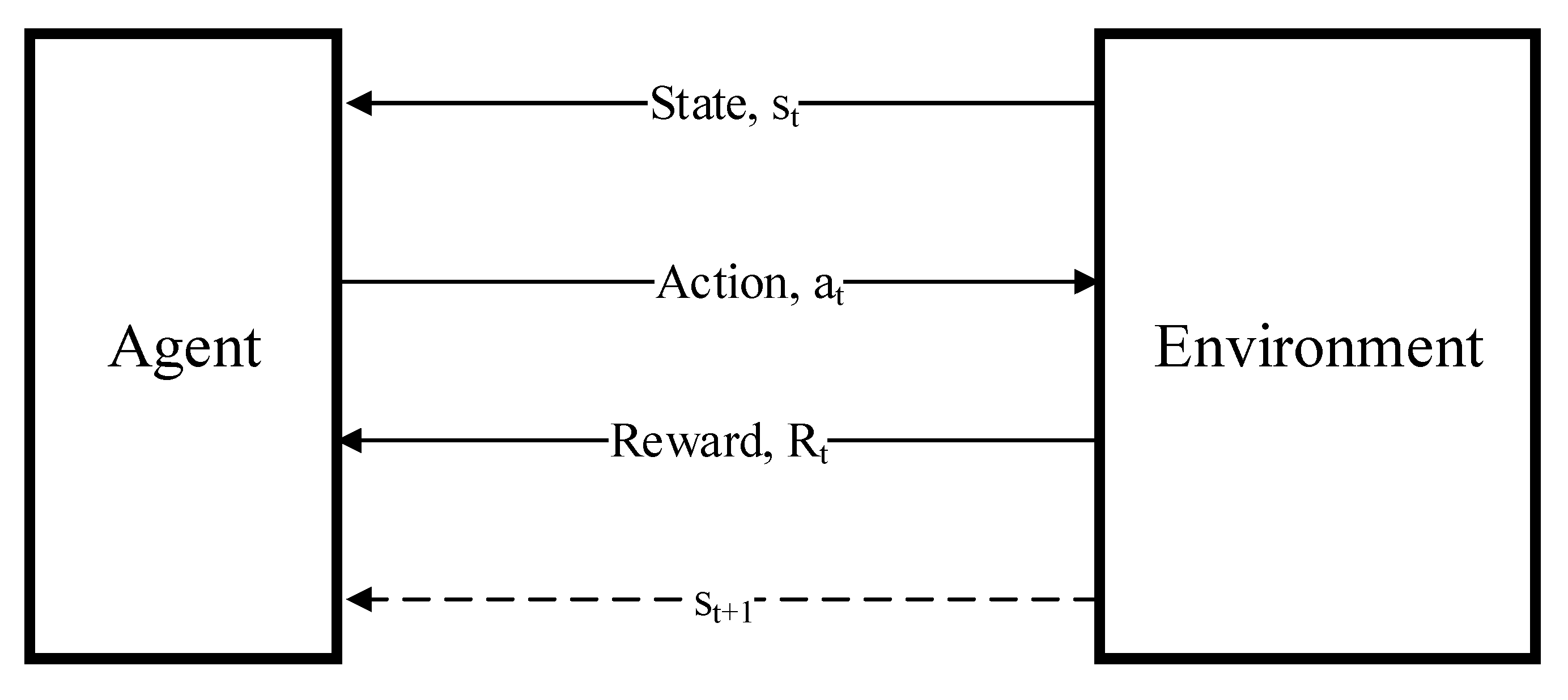
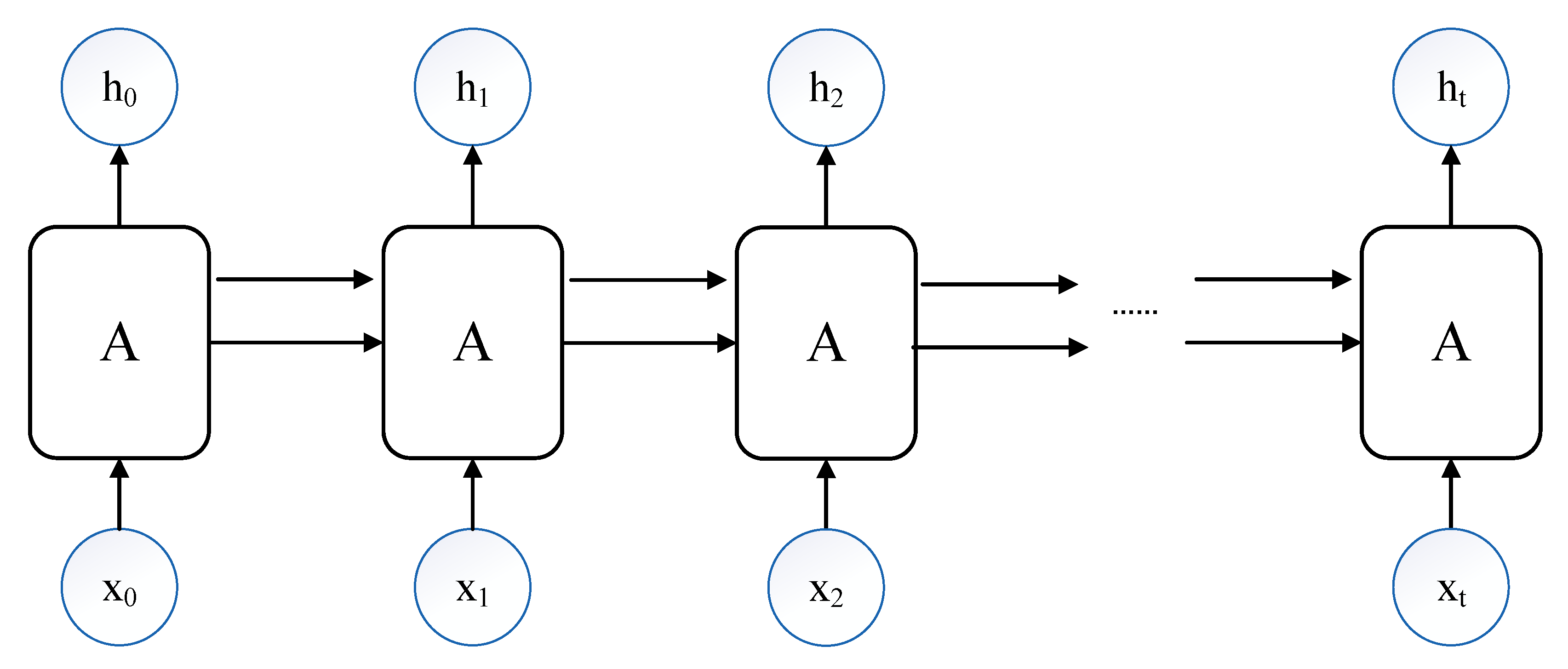
2.1. Reinforcement Learning

RL is an adaptive machine learning method, which aims to optimize the decision-making based on the evaluation of the environmental feedback signal [7]. Agent and environment are the two main elements in RL. In an HVAC problem, the environment (controlled system) is all those indoor and outdoor factors that influence a room or zone of the building, and the agent is a decision maker to manage a room or zone actuators of the building, according to specified setpoints [6].

Besides agent and environment, RL also includes some basic elements. A state (short for $s$) is the description of the environment and the agent. An action (short for $a$) is the description of the behavior of agent. A policy $\pi \left(a|s\right)$ is the function of action that agent determines based on the state $s$. A reward $R$ is a measure of the action that environment feeds back to the agent after the agent has made the action based on the state $s$.

As shown in Figure 1, each time step the agent takes action $a_t$ to interact with the environment based on state $s_t$. Environment gives the agent reward $R_t$ and next state $s_{t+1}$, usually a bigger reward means a better action. The agent adjusts the policy according to the reward.

A return $G$ is the accumulation of each moment (step) reward from the moment of t to the end of episode. The mathematical expression of return $G_t$ is shown as Equation (1).

$$G_t=R_t+\gamma R_{t+1}+{\gamma }^2{R}_{t+2}+......={\displaystyle \sum _{k=0}^n{\gamma }^k{R}_{t+k}}$$

(1)

where $G_t$ is a return following time step $t$; $\gamma$ is a discount factor, a number between 0 and 1, which is introduced because of rewards work differently at each moment.

A state value $V_{\pi }(s)$ represents the expectation of the return that agent can obtain in a state based on a given policy $\pi$ shown as Equation (2).

$$V_{\pi }(s)=E_{\pi }\left[G_t|s_t=s\right]$$

(2)

An action value $Q_{\pi }(s,a)$ represents the expectation of the return that agent can obtain by taking action $a$ in state $s$ based on a given policy shown as Equation (3).

$$Q_{\pi }(s,a)=E_{\pi }\left[G_t|s_t=s,\hspace{0.33em}{a}_t=a\right]$$

(3)

2.2. SAC

Soft actor-critic (SAC) algorithm is an off-policy actor-critic DRL algorithm based on the maximum entropy RL framework. In this framework, actor is designed to maximize the expected return and entropy. This ensures greater exploration capabilities of the algorithm while completing tasks. By combining an off-policy update with an actor-critic framework, the stability of the algorithm is guaranteed. Meanwhile, the use of off-policy provides a better data efficiency.

The SAC algorithm is developed based on policy iteration (PI) in two steps. In step 1, Policy Evaluation is used to evaluate the quality of a policy using state value function $V(s_t)$. In step 2, Policy Improvement is used to update the policy $\pi \left(a_t|s_t\right)$. There are several ways to update the policy. To improve the exploration ability, SAC has transformed policy iteration into a soft policy iteration process. In the policy evaluation step, entropy is added to construct the soft state value function $V(s_t)$ shown as Equation (4).

$$V(s_t)=E_{a_t\sim \pi }[Q(s_t,a_t)-\log \pi (a_t|s_t)]$$

(4)

The soft action value function $Q(s_t,a_t)$ is constructed based on $V(s_t)$ and shown as Equation (5).

$$Q(s_t,a_t)=r(s_t,a_t)+\gamma E_{s_{t+1}\sim p}[V(s_{t+1})]$$

(5)

Unlike previous policies of certainty in the policy update process, soft policy iteration $J_{\pi }$ aligns the distribution of the policy $\pi (a_t|s_t)$ with the distribution of the soft action-value function $Q(s_t,a_t)$, shown as Equation (6), i.e.,

$$J_{\pi }=D_{KL}(\pi (a_t|s_t)||\frac{\exp (Q(s_t,a_t))}{Z(s_t)})$$

(6)

$D_{KL}$ is the Kullback–Leibler divergence used to evaluate the difference between two probability distributions. The partition function $Z(s_t)$ is used to normalize the distribution.

After an operation, the target function of a policy update can be equivalent, which determines the importance of entropy relative to the reward, then controls the randomness of the policy. Since the policy is a distribution that is based on sampling, the above formula cannot be derived, so a reparameterization trick is used to sample the action: $a_t=f({\epsilon }_t;s_t)$, where ${\epsilon }_t$ is a Gaussian distribution. In this way, the integration of action in the policy objective can be converted into integrals, shown as Equation (7).

$$J_{\pi }=E_{{\epsilon }_t\sim N}[\alpha \log (\pi (f({\epsilon }_t;s_t)|s_t))-Q(s_t,f({\epsilon }_t;s_t))]$$

(7)

$\alpha$ is the temperature parameter to control the stochasticity of the optimal policy.

2.3. Online Learning

Online learning refers to the usage of real-time data (or data block) by a model for training or optimization so that the model has better predictive performance with future data [25,26]. There are more restrictions on online learning than offline learning methods [27,28]. Due to the lack of data at the beginning of online learning, memory allocation and the structure of a model cannot be completed in advance. Meanwhile, the processing time in online learning is limited. The processing needs to be completed before new data arrive. Data during different periods are non-stable. There may be conceptual drifts that require real-time maintenance of the model.

With the success of deep learning applications, more and more online learning scenarios are using deep learning to solve related problems. Due to the limitations of online learning, deep learning applications in the field of online learning require the ability to self-adjust. It means the parameters and structure of the network can be modulated based on new coming data [29]. Therefore, the problem can be divided into three aspects: timing of starting the adjustment, the way of network parameter adjustment, and the way of model structure adjustment.

There are more in-depth studies for the latter two aspects already. The network parameter adjustment mainly includes three methods: sample selection [30,31], sample weight [31,32], and model structure [33,34]. The model structure adjustment mainly includes constructive algorithms [35], pruning algorithms [36], hybrid algorithms [37], and regularization techniques [38]. In the past ten years, studies of online deep learning have been deepened, but the proposed methods were more generalized, not considering the data characteristics of HVAC systems.

3. Framework of Proposed Algorithm

3.1. Problem Definition

The optimal control problem of an HVAC system can be summarized as finding a corresponding control policy to make the accumulated system energy consumption in a period of time as small as possible while satisfying the indoor temperature demand, as:

$$\begin{array}{l}{\min }_{\pi *(a|s)}{\displaystyle \sum _{t=0}^{T}power(t)}\\ \hspace{0.33em}\hspace{0.33em}\hspace{0.33em}\hspace{0.33em}s.t.\hspace{0.33em}\hspace{0.33em}{c}_i(t)\le 0\\ \hspace{0.33em}\hspace{0.33em}\hspace{0.33em}\hspace{0.33em}\hspace{0.33em}\hspace{0.33em}\hspace{0.33em}\hspace{0.33em}\hspace{0.33em}{c}_i(t)=\left\{\begin{array}{c}{T}_i(t)-{\lambda }_i(t),\hspace{0.33em}\hspace{0.33em}\hspace{0.33em}\hspace{0.33em}\hspace{0.33em}\hspace{0.33em}\hspace{0.33em}\hspace{0.33em}cooling\hspace{0.33em}\hspace{0.33em}\\ {\lambda }_i(t)-T_i(t),\hspace{0.33em}\hspace{0.33em}\hspace{0.33em}\hspace{0.33em}\hspace{0.33em}\hspace{0.33em}\hspace{0.33em}\hspace{0.33em}heating\end{array}\right.\hspace{0.33em}\hspace{0.33em}\hspace{0.33em}\hspace{0.33em}i=1,2,......N\end{array}$$

(8)

${\pi }^{*}(a|s)$ is the optimal policy; $power(t)$ is the total energy consumption of HVAC system at time t; $T_i(t)$ and ${\lambda }_i(t)$ are the actual temperature and set temperature of the i-th zone in the building at time t, respectively; $N$ is the total number of zones.

According to our exploration of the HVAC system control, under different energy supply modes and system working mechanisms, the corresponding relationships between consumed power and indoor demand satisfaction of the same control policy are shown as Figure 2.

It is generally believed that the greater the system power consumed, the more it can meet the indoor demand, and vice versa. Generally, it is mainly divided into three policy forms.

As show in policy 1 in Figure 2, when the system is controlled at low power, it cannot meet the minimum indoor demand; with the gradual increase in power, the indoor demand is met; when the system is under high power, it may far exceed the indoor demand, resulting in a waste of energy. In some cases, as show in policy 2, low power consumption can meet the indoor demand, so the energy-saving space is large. However, as shown in policy 3, sometimes it is necessary to consume high power to meet the indoor demand, so it will be difficult to save energy consumption.

Therefore, the optimal control policy of the HVAC system is to minimize the power consumption in the long term and on the premise of meeting the indoor demand. It is consistent with the learning goal of safe RL, which is to maximize the long-term return under safety constraints.

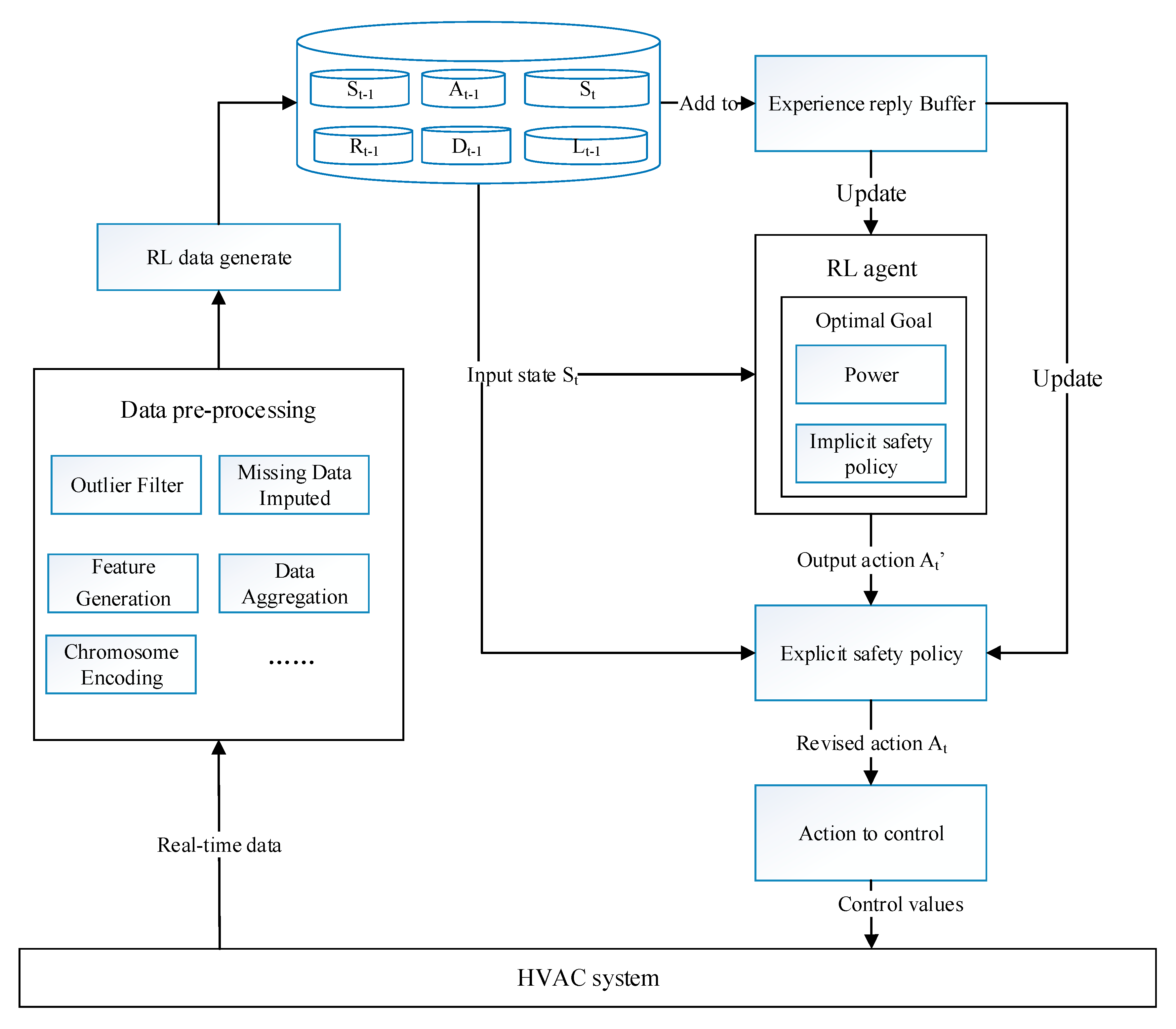
3.2. Framwork Overview

RL with dual safety policies for energy savings in an HVAC system consists of three main modules. They are data pre-processing, RL model and explicit safety policy. The schematic diagram of the proposed algorithm is shown as Figure 3.

The data pre-processing module processes the data collected by the HVAC system and extracts valid information. At the same time, the feature data uploaded at different times are organized into a regular data form for the algorithm to store and use.

Pre-processed data will be generated and added to the experience reply buffer, for parameter updating of the RL and explicit safety policy. Among them, the temperature labels $L_t\in \{0,1\}$ indicate whether the indoor temperature exceeds the safety boundary. The safety boundary is generally composed of the temperature value set by the user and the safety range. The purpose of the safety range is to avoid the abnormal situation that the temperature value set by the user cannot be satisfied due to the property limitation of the system.

Implicit safety policy is a part of the RL model, which integrates safety into the optimization goal of RL. It adds penalties for actions that exceed the safety constraints (reward shaping) to improve the reward into two sub-tasks, power-related and safety-related. By training, it makes the RL model learn not only the optimal but also the safer policy.

The explicit safety policy module determines the action outputted by RL in real time to ensure the safety. The RL model outputs the basic action according to the current state. If the action meets the demands of the indoor temperature, the HVAC system will be controlled based on the action. Otherwise, it needs to traverse the action space to select all legal actions and generate a set of alternative actions. The best action is then selected from the set of alternative actions by some rules. When the set of alternative actions is empty, a default action with the maximum system power is given based on prior knowledge. In this paper, the basic RL algorithm uses the SAC algorithm.

3.3. Data Pre-Processing

3.3.1. Data Pre-Processing Introduction

The data pre-processing module processes the data collected by an HVAC system. Due to the different data sampling frequencies in the system, the data cannot be uploaded at the same time. Therefore, the data need to be aligned in the time dimension first. The module fills or aggregates data according to different sampling rules, identifies and processes outliers according to data characteristics and the upper and lower limits set by prior knowledge, uses relevant data for mutual verification to deal with data conflicts, and generates new features. Finally, the useful information in the sampling period is integrated into regular data for use in subsequent steps.

3.3.2. Settings of Reinforcement Learning

The energy-saving control problem of HVAC fits the basic theory of the reinforcement learning algorithm, so the SAC algorithm can be used to solve this problem. Based on SAC basic principles, State (s), Action (a), and Reward (r) are three fundamental elements, which need to be defined.

State: State consists of three typical categories: indoor and outdoor air temperatures and relative humidity, status of devices, and key operating parameters of equipment. The status of devices is represented by $\{0,1\}$ as Boolean parameter. When the performance and power of devices are similar, the amounts of devices turned on are used to reduce the dimension of the state, which can speed up the exploration efficiency of the algorithm. Even some devices cannot be controlled by the algorithm; their parameters have a critical impact on the indoor temperature and energy consumption. Therefore, these parameters should be used in the algorithm as a key state.

Action: Action space is selected based on an actual scene. Theoretically, the action space should be larger than the optimal space to ensure that RL can explore the optimal policy. However, for the sake of device safety, the range of action will be limited, so the optimal action space is smaller.

Reward: The reward is shown as Equation (9).

3.4. Implicit Safety Policy

The RL agent is designed to generate the lowest energy consumption but safe actions. Therefore, the optimization goal of RL should not only include the consumed power of the HVAC system but also the safety constraints. It is a feasible way to design the composition of reward by penalizing unsafe actions. So far, the reward function has two forms. The first function is to reduce the total system power consumption as much as possible within a certain period. The second function punishes unsafe actions by adding a penalty value. The reward function is shown as follows:

$$R_t=\left\{\begin{array}{c}-{\displaystyle \sum _{t=1}^{T}P(t),\hspace{0.33em}\hspace{0.33em}\hspace{0.33em}\hspace{0.33em}\hspace{0.33em}\hspace{0.33em}\hspace{0.33em}\hspace{0.33em}\Delta T_{\max }(t)\le 0}\\ -{\displaystyle \sum _{t=1}^{T}P(t)-\alpha \Delta T_{\max }(t),\hspace{0.33em}\hspace{0.33em}\hspace{0.33em}\hspace{0.33em}\hspace{0.33em}\hspace{0.33em}\hspace{0.33em}\hspace{0.33em}\Delta T_{\max }(t)>0}\end{array}\right.$$

(9)

Among them, $P(t)$ represents the total power consumption of the HVAC system at timestep $t$; $\Delta T_{\max }(t)$ represents the maximum value at which the room exceeds the set temperature in the control period t. $\alpha$ is the weight of $\Delta T_{\max }(t)$ to balance the values of $\Delta T_{\max }(t)$ and $P(t)$. The calculation method is slightly different in the heating mode compared to that used in the cooling mode of the HVAC system.

3.5. Explicit Safety Policy

The implicit safety policy learns safety policy by adding penalties in reward for unsafe actions. However, this method requires the algorithm to explore and learn for a long time, and cannot guarantee real-time safety. Therefore, we propose an explicit safety policy algorithm based on online residual learning, which can construct a safety classifier to filter out unsafe actions and select the optimal safe action.

Explicit safety policy algorithm mainly consists of two components, an online safety classifier, alternative action collection and optimal action selection. The online safety classifier is built to predict whether the action taken by RL will result in indoor temperature dissatisfaction, and it is trained with the data sampled from experience reply buffer. If the action outputted by RL is classified as unsafe action, the mechanisms of alternative action collection generation and optimal action selection will be triggered. All actions identified by online safety classifier as meeting the indoor temperature constraints constitute an alternative action collection. The best action that maximizes the benefit in all alternative actions could be selected by some rules.

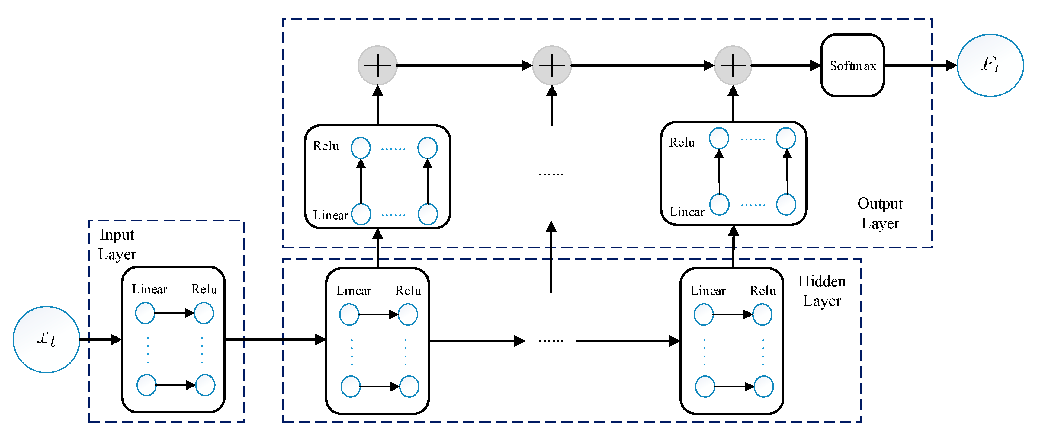
3.5.1. Online Safety Classifier

The online safety classifier solves a binary classification problem. The goal is to learn the corresponding mathematical relationship $F:X\to Y$, from streaming data $\left(x_t,y_t\right)$. $x_t\in R_d$ is a sample for $d$ dimension features. $y_t\in \left\{0,1\right\}$ is a classification label. ‘0′ indicates that all indoor air temperatures are meet demand, and ‘1′ indicates that there is indoor air temperature not meet demand. The binary classifier is constructed with neural network. In an HVAC system, the current state is largely dependent on the previous state. So, indoor air temperature dissatisfaction is selected as a start signal to adjust the classifier network. When the classifier prediction result is correct, the network is believed to be reasonable. When the prediction result is incorrect, it is highly likely that future predictions will be incorrect, so the network needs to be adjusted.

Based on the idea of dynamic adjustment of network structure, the network based on residual learning is proposed. The network structure of model is shown in Figure 4.

The online safety classifier’s network structure is similar to LSTM (long short-term memory) and an output layer is added to each hidden layer, then the results of all output layers are added. LSTM has been successfully applied to power consumption forecasting [39] and energy saving [40]. The main structure of LSTM is shown in Figure 5.

In Figure 5, $x_0,x_1,x_2,......,x_t$ are the inputs at time $0,1,2,......t$; $A$ is an LSTM unit, which is constructed by different components with one memory cell and four gates (input, forget, cell, and output) [41]. $h_0,h_1,h_2,......h_t$ are outputted by $A$, which represent the hidden state of time $0,1,2,......t$.

Supposing the network includes $N$ hidden layers, the prediction process of a new sample $x_t$ is shown by the blue arrows in the network structure in Figure 4. The details are shown as Equation (10):

$$\begin{array}{c}F(x_t)=\arg \max ({\displaystyle \sum _{n=0}^N{f}^{(n)}})\\ f^{(n)}={\sigma }_1({\Theta }^{(n)}{h}^{(n)})\\ \hspace{0.33em}\hspace{0.33em}\hspace{0.33em}\hspace{0.33em}{h}^{(n)}=\left\{\begin{array}{c}{x}_t,\hspace{0.33em}\hspace{0.33em}\hspace{0.33em}\hspace{0.33em}\hspace{0.33em}\hspace{0.33em}n=0\\ {\sigma }_2(W^{(n)}{h}^{(n-1)}),\hspace{0.33em}\hspace{0.33em}\hspace{0.33em}\hspace{0.33em}n>0\end{array}\right.\end{array}\hspace{0.33em}\hspace{0.33em}\hspace{0.33em}\hspace{0.33em}\hspace{0.33em}\hspace{0.33em}\hspace{0.33em}$$

(10)

${\sigma }_1$ and ${\sigma }_2$ are activation functions. They can be different activation functions. $W^{(n)}$ is the weight of the hidden layers. ${\Theta }^{(n)}$ is the weight of the output layers.

A typical process for a binary classification problem for a new sample is to predict the classification to which the new sample belongs. Then, a loss value, such as cross-entropy, is calculated. Finally, the network parameters are updated by the backward algorithm. Unlike this process, the residual learning approach to update network parameters is proposed in this article. The main differences are as follows:

• If a network consists of $N$ hidden layers, each layer will correspond to an output layer, and each output layer’s learning objectives are not the same. For the layer $n$, the learning objective is $f^{(n)}=y_t-{\displaystyle \sum _{i=0}^{n-1}{f}^{(i)}}$. In this way, different network structures can be implemented.

• The parameters of network are not updated simultaneously with backward propagation. The parameters of each hidden and output layer are updated layer by layer. When the parameter of a layer is updated, a new sample is required to update the shallow network. The updating formula is listed as follows in Equations (11) and (12).

$${\Theta }_{t+1}{}^{(n)}={\Theta }_t{}^{(n)}-\eta {\nabla }_{{\Theta }_t{}^{(n)}}L(f^{(n)},\hspace{0.33em}{y}_t-{\displaystyle \sum _{i=0}^{n-1}{f}^{(i)}})$$

(11)

$$W_{t+1}{}^{(n)}=W_t{}^{(n)}-\eta \prime {\nabla }_{W_t{}^{(n)}}L(f^{(n)},\hspace{0.33em}{y}_t-{\displaystyle \sum _{i-0}^{n-1}{f}^{(i)}})$$

(12)

where $\eta$ and ${\eta }^{\prime }$ are learning rate. $L$ is loss function, and the MSE is used in this design.

3.5.2. Alternative Action Collection Generation and Optimal Action Selection

The generation of alternative action collection needs to be realized with the help of an online safety classifier to verify whether the action will meet the indoor temperature demand in a given state. When the action is continuous, it needs to be discretized. The degree of discretization needs to be determined in practical scenarios.

After the collection of alternative actions is generated, in order to select the best actions, the benefits from corresponding action should be considered. That is the long-term return of action $a$ in given state $s$. In RL, action value function can solve this problem. In this design, in order to take into account the maximum entropy principle of the SAC algorithm and ensure the exploration ability of the algorithm, the following definitions are adopted.

$$A^{\pi }(s,a)=Q^{\pi }(s,a)-\log \pi (a|s)$$

(13)

where $\pi$ is the policy, $Q(s,a)$ is an action value function.

Algorithm 1 depicts the main working process of explicit safety policy.

Algorithm 1. Explicit safety policy

Input: Learning rate parameter $\eta ,\hspace{0.33em}\hspace{0.33em}{\eta }^{\prime }$ Initialize: $F(x)$ with $N$ hidden layers and ${\theta }^n,\hspace{0.33em}{W}^n\hspace{0.33em}\hspace{0.33em}n=1,2,......N$ 1. for $t=1,2,......T$ do 2.   Receive instance $x_t$; 3.   Predict ${y\prime }_t=F(x_t)$; 4.   If ${y\prime }_t==1$ then 5.     Obtain alternative action collection; 6.     Obtain best action; 7.   Obtain true label $y_t$; 8.   If ${y^{\prime }}_t\ne y_t$ then 9.     for $n=1,2,......N$ do 10.      Predict ${f_{old}}^{(n)}$; 11.      Calculate Loss $L({f_{old}}^{(n)},\hspace{0.33em}{y}_t-{\displaystyle \sum _{i=0}^{n-1}{f_{new}}^{(i)}})$; 12.      Update ${\theta }^{(n)},\hspace{0.33em}{W}^{(n)},\hspace{0.33em}{h}^{(n)}$; 13.      Update ${f_{old}}^{(n)}$ to ${f_{new}}^{(n)}$ with ${\theta }^{(n)},\hspace{0.33em}{W}^{(n)}$; 14. end

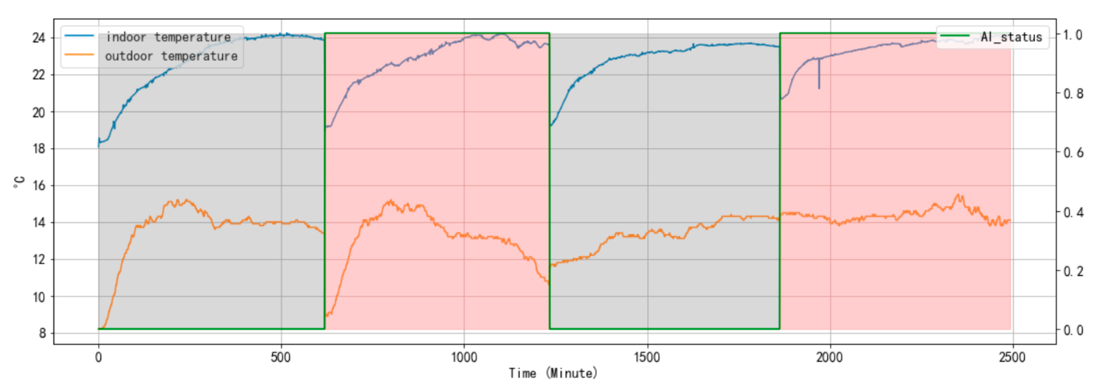
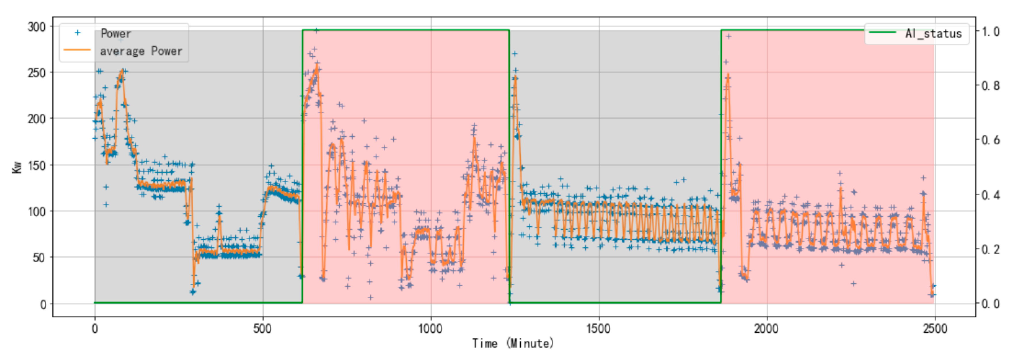
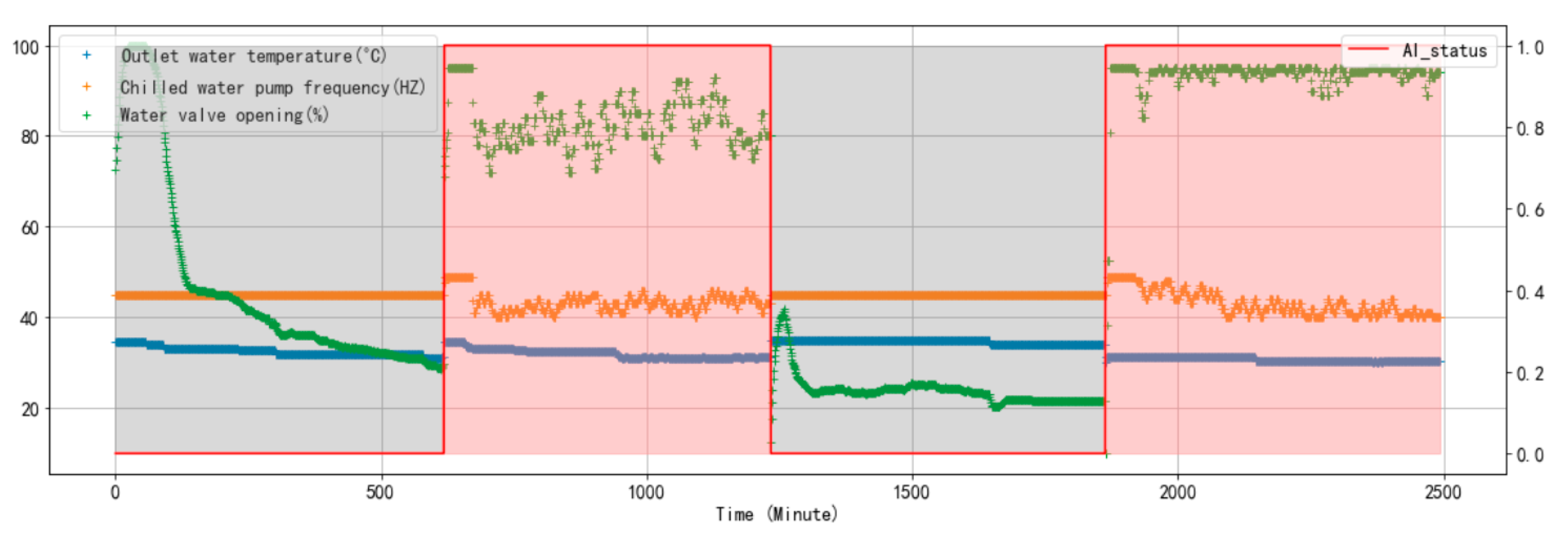
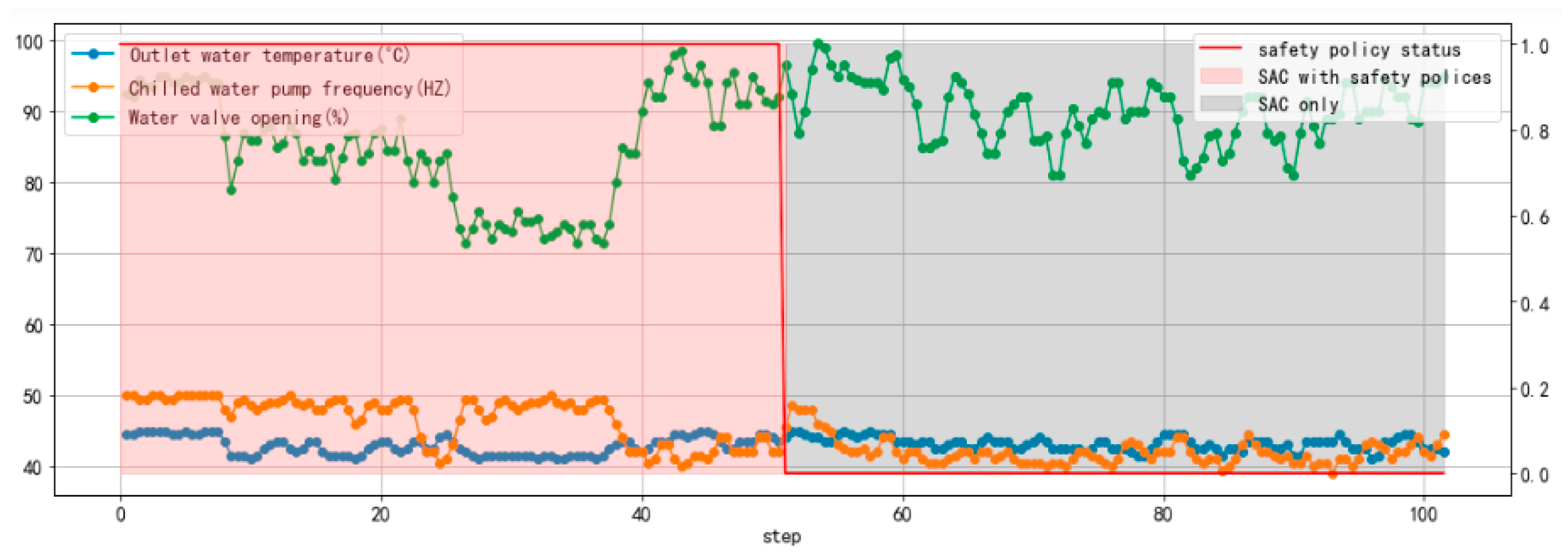
4. Results and Discussion

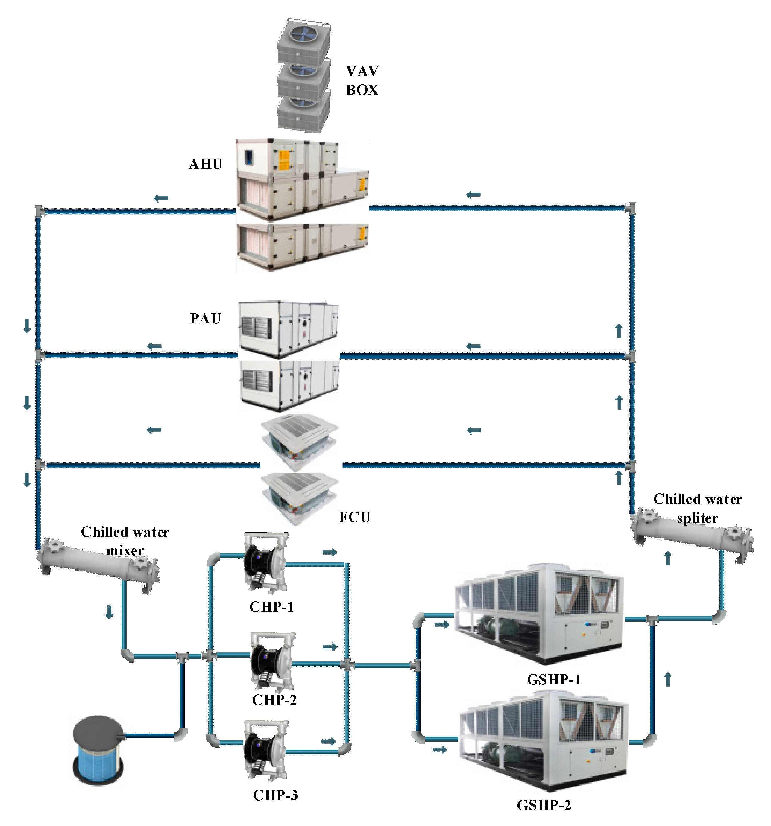
4.1. Case System

4.1.1. System Structure

To verify the effectiveness of the control algorithm, we conduct experiments in a real commercial building. This building is a retrofit commercial building including office, exhibition hall, conference center, and cafeteria area. The building has five floors with a total floor area of about 9000 m². The ratio of window and envelop is about 30%.

Table 1. Building properties of the test building.

Space	Structure	Material Type or Schedule
Envelop	Exterior wall	Hollow bricks wall
	Window	Dual-glazed windows
	Floor	Concrete
Schedule	Occupancy schedule	7:30 am to 5 pm on weekdays Closed on weekends
	HVAC schedule	7 am to 5 pm on weekdays Closed on weekends

shows the properties of this commercial building.

The open schedule of this building is from 7:30 am to 5 pm on weekdays, and the building is closed during weekends. There are around 200 persons working in this building. The operation period of the HVAC system of this building is from 7 am to 5 pm on weekdays, and the building is closed on weekends. The systems are turned on if there are people working overtime.

The HVAC system of this building includes typical water and air systems. The chilled water system consists of two heat pumps and three primary chilled water pumps. The air system consists of 11 AHUs, 118 VAV boxes, 3 PAU units and 6 FCU units. Each AHU serves several VAV boxes, and each VAV box corresponds to the sensor that measures the indoor air temperature. The HVAC system schematic diagram of this building is shown in Figure 6. Under normal operation mode, the status of the water system is stable, and one heat pump and two primary chilled water pumps are turned on.

The state space and action space of the implemented RL algorithm in this HVAC system are shown in

Table 2. State space for the implemented RL algorithm.

Space	Parameters
States	Outdoor air temperature
	Outdoor relative humidity
	Status of heat pumps, AHU, PAU, FCU and VAV box
	Frequencies of AHU, PAU and FUC
Actions	Setting temperature of heat pump outlet water
	Setting frequency of Primary chilled water pump
	Setting opening of AHU water valve

.

4.1.2. System Characteristics

In order to better analyze the performance of the proposed algorithm, we explored the characteristics of the HVAC system in advance to obtain the operation logic of the HVAC system, mainly the influence of action and key state factors on system power and indoor air temperature. We conducted a two-week test in heating mode, and then conducted partial correlation analysis on the collected data using Spearman coefficient. The results are shown in

Table 3. Partial correlation coefficient among system factors.

Factors	Heat Pump Power	Primary Chilled Water Pump Power	AHU Power	System Power	Indoor Temperature
Heat pump outlet water temperature	0.52	0.24	0.20	0.44	0.14
Primary chilled water pump frequency	−0.16	0.75	0.05469	−0.0	0.08
AHU water valve position	0.17	0.24	−0.20	0.17	0.46
Outdoor temperature	0.25	−0.07	0.29	0.30	0.52
Outdoor humidity	0.18	0.11	0.13	0.25	0.32

. The null hypothesis of the correlation analysis is that there is no association between the two random variables. The result of the black background indicates that the calculated p-value is greater than 0.05, and the hypothesis is accepted, that is, the primary chilled water frequency has little significant effect on the system power.

When the number of devices on and the key operating parameters of uncontrollable equipment are determined, according to Table 3: (1) the power of the heat pump is mainly affected by the water outlet temperature of the heat pump, and the higher the water outlet temperature, the greater the pump power, and vice versa; (2) the power of the primary chilled water pump is mainly affected by the frequency of the primary chilled water pump, and the higher the frequency, the greater the power, and vice versa; (3) the power of AHU is mainly affected by outdoor temperature, but it does not show significant influence; (4) system power is mainly affected by the outlet water temperature and outdoor temperature, and the frequency of the primary chilled water pump and the AHU water valve position have little influence on the system power; (5) indoor temperature is mainly affected by the AHU water valve position and outdoor temperature, which are positively correlated with both. In addition, in order to be consistent with the actual application, PAU and FCU were not turned on during this test.

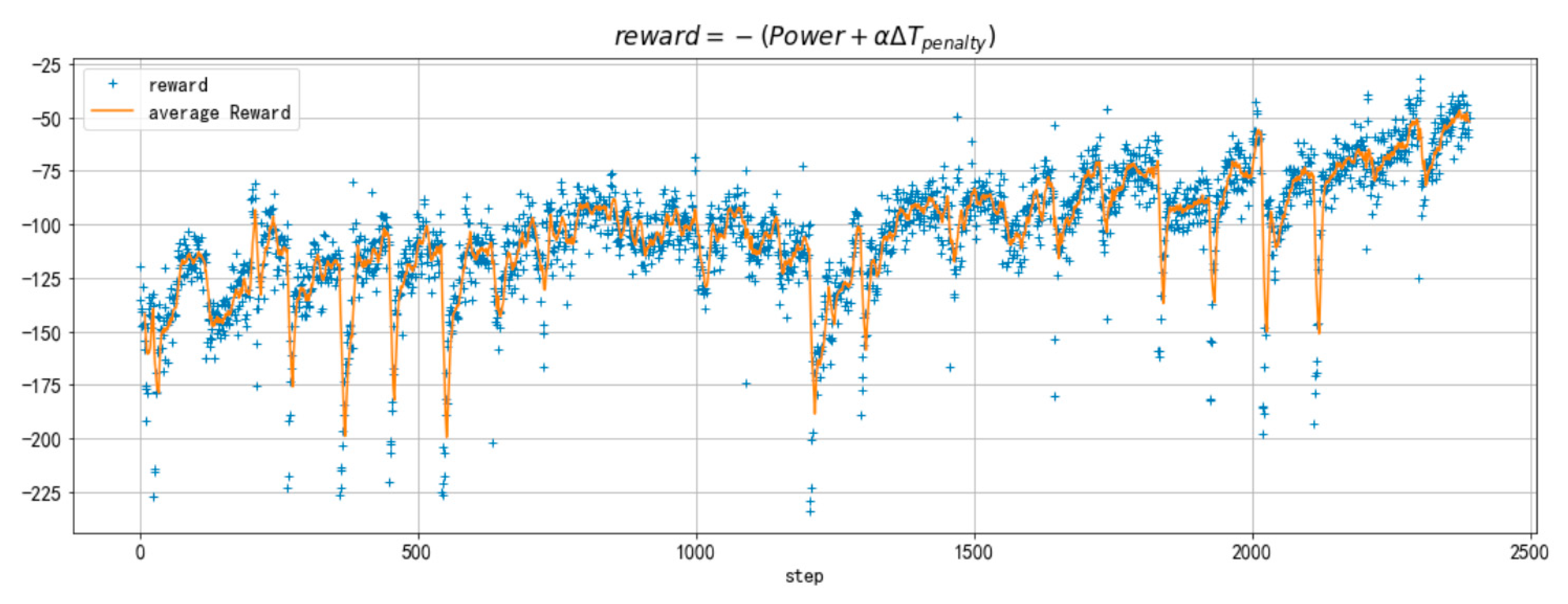
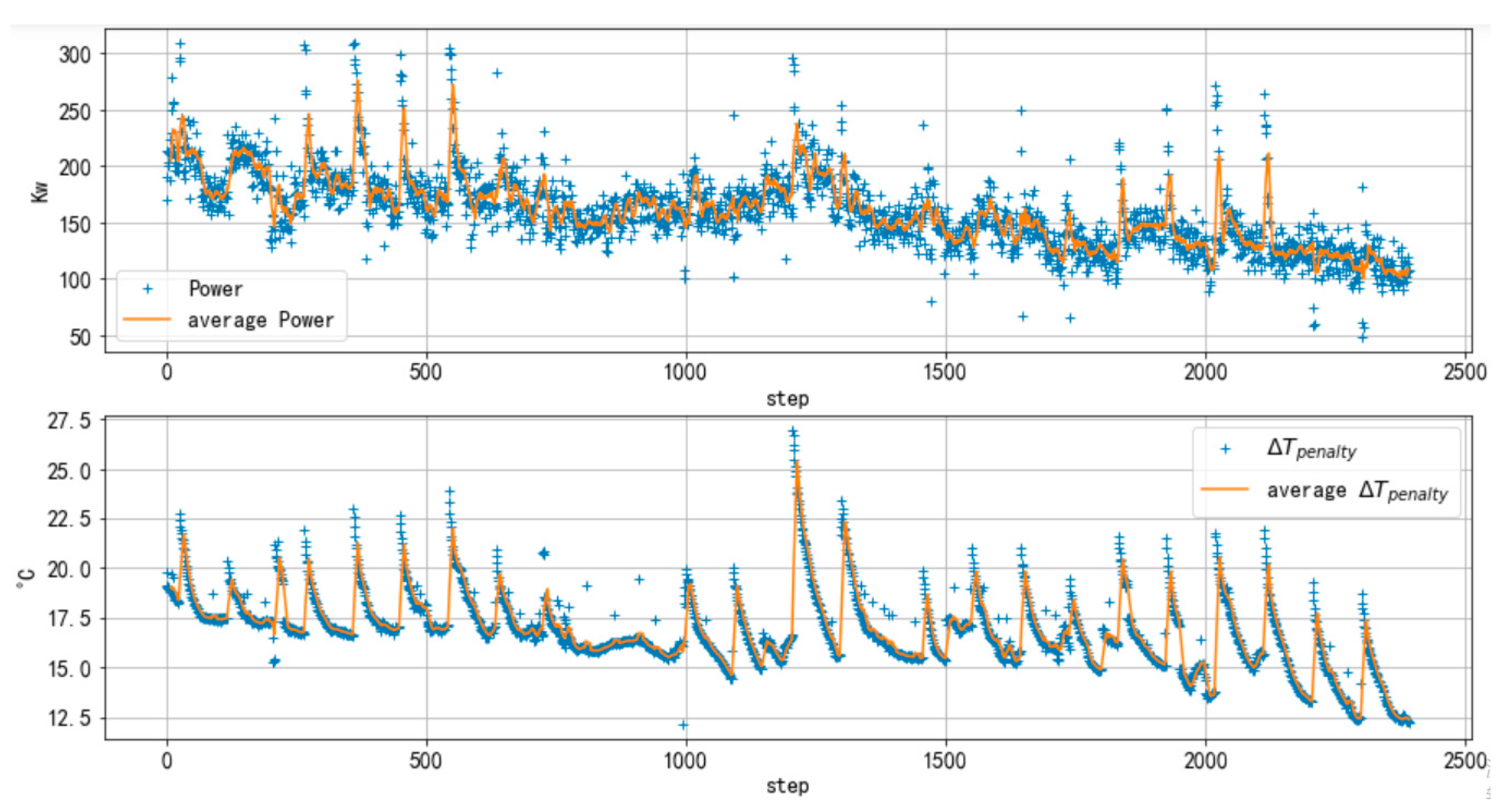
4.2. Effectiveness of Proposed Algorithm

4.2.1. Overview

The proposed control algorithm is deployed in a real commercial building, to verify the effectiveness. Data during the controlling of building automation system (BAS), which is the original control system of HVAC, are collected, analyzed and compared as a baseline case. Based on the data of BAS control, the effectiveness of the proposed control algorithm could be illustrated from the perspectives of reward, action convergence, and energy saving by AB testing. The AB test is a common method to evaluate the control performance of different control algorithms. By applying algorithm A and B, respectively, in similar system environments, the performance of each algorithm will be tested. In our scenario, “A” represents AI control, that is, our proposed control algorithm; “B” represents BA control, that is, original BAS control algorithm.

When the system is operated with the proposed control algorithm, the outdoor temperature ranges from 4.10 to 28.00 °C, and the average indoor temperature ranges from 14.90 to 23.91 °C. The reward changing trend is shown in Figure 7, and the power consumption and indoor temperature penalty trends of the proposed RL algorithm are shown in Figure 8.

The RL takes approximately 2400 steps during the whole control process, and the algorithm operating cycle (each step) of the proposed algorithm is set as 12 min. The system runs approximately 10 h a day when the system is controlled under the proposed algorithm. It takes approximately 20 days when the reward of the RL algorithm is stabilized and converged.

In order to obtain reliable energy-efficient verification data, two phases of AB tests are token, and the results are shown in

Table 4. AB test details.

Phase	Date	Average Indoor Temperature	Average Outdoor Temperature	Control Method	Energy Saving Rate
test1	3 February 2021	21.71 °C	13.54 °C	BA	6.51%
	4 February 2021	22.33 °C	13.11 °C	AI
test2	12 March 2021	22.21 °C	13.30 °C	BA	15.02%
	16 March 2021	22.62 °C	14.39 °C	AI

. Here, one phase represents the period from the beginning of BA control to the end of AI control, with only one control mode switch.

The first phase (test 1) is in the first week when the algorithm is implemented, and the second phase (test 2) is in the last week when system runs under the proposed algorithm. Under BA case, the HVAC system is still controlled with the PID controller, and the PID parameter is set as the original. Therefore, the chilled water outlet temperature is set constant at 45 °C, and the frequency of primary chilled water pumps is set constant at 45 Hz. The valve position of AHU is controlled by the supply air temperature of AHU using the PID controller.

It is found that the average outdoor air temperature during phase 1 is 0.43 °C lower than that during the baseline case. During phase 1, the average indoor air temperature is 0.62 °C higher and the power consumption is reduced by 6.51%, compared to the baseline case. During phase 2, the outdoor air temperature is 1.09 °C higher and the average indoor air temperature is 0.41 °C higher, and the electricity consumption reduction is 15.02%, compared to the baseline case. In the early stage of the algorithm, the energy efficiency is relatively low, and the energy efficiency increases along with the learning of the proposed algorithm.

The indoor temperature, outdoor temperature, system power consumption and action values during two AB test phases are shown in Figure 9, Figure 10 and Figure 11. In the figures, left coordinate axes represent the values of temperature, power and actions. The right coordinate axis shows the value of AI_status, which indicates the running status of the AI algorithm. When AI_status is 0, it represents that the HVAC system is under BA control mode (gray shaded area in figures). When AI_status is 1, it means that the HVAC system is controlled by our proposed algorithm (the red shaded area in the figure).

As can be seen from figures, the indoor temperature and outdoor temperature during two AB test phases are almost in the same range. The actions of test 2 are significantly more stable than that of test 1.

During test 2, the heat pump outlet water temperature is controlled at the minimum value, and the water valve position of AHU is controlled at the maximum value, and the demand is met by modulating the primary chilled water pump frequency. It shows that the proposed algorithm can learn the system characteristics after a period of learning and provide reasonable action of the system.

4.2.2. Performance of Online Safety Classifier

To evaluate the performance of the online safety classifier algorithm with the increase in data amount, all of the data are divided into three phases. The first 300 rounds of learning is labeled as a mid-phase; the first 1000 rounds of learning is labeled as a late-phase. The entire process of training is labeled as entire phase. The accuracy and recall rate results are shown in

Table 5. Performance of increased data amount for online safety classifier.

Metric	Mid-Phase	Late-Phase	Entire Phase
precision	0.91	0.945	0.937
recall	0.75	0.78	0.774

. During the entire learning process, the performance of the algorithm does not fluctuate significantly with the increase in data amount.

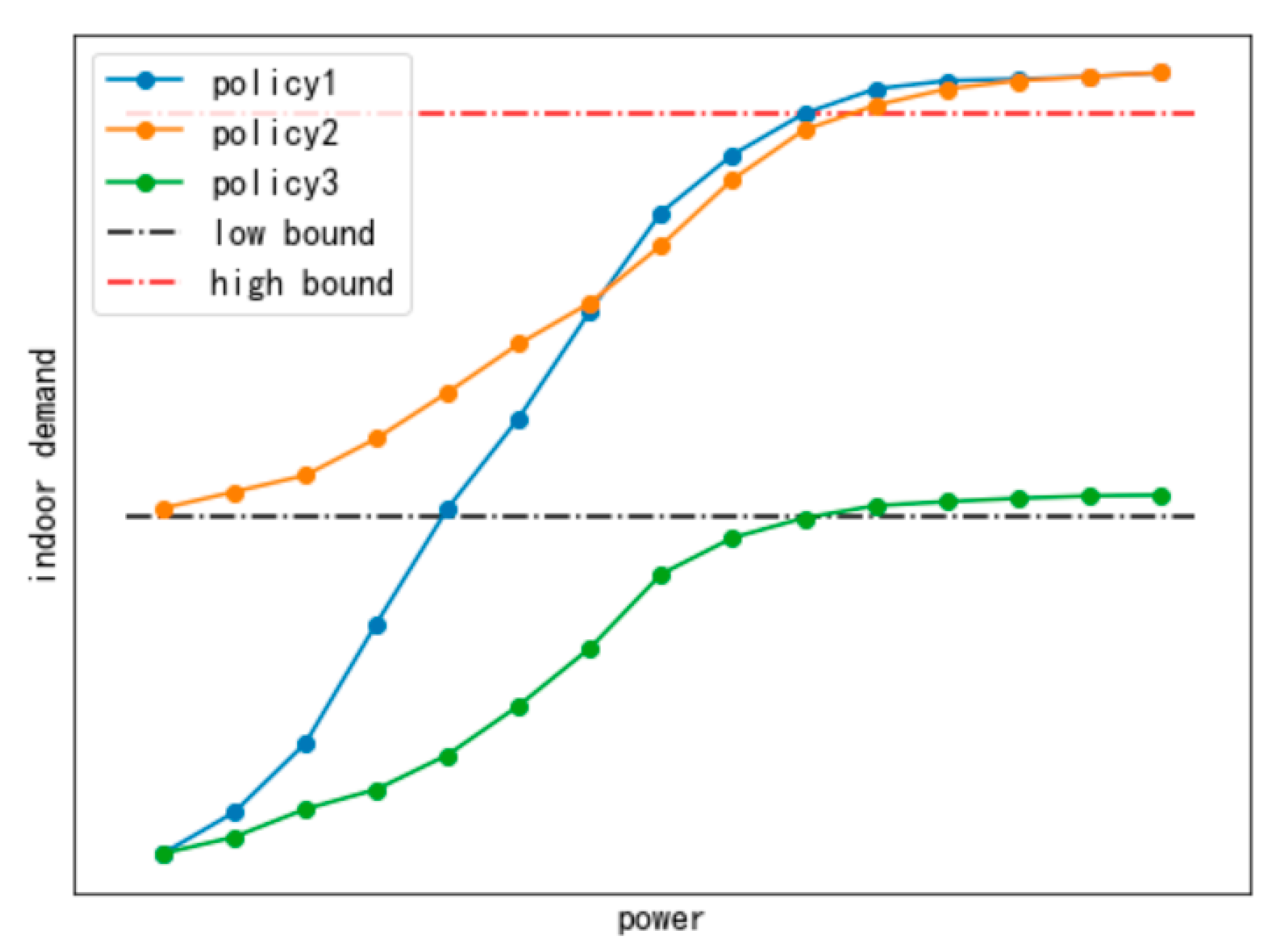
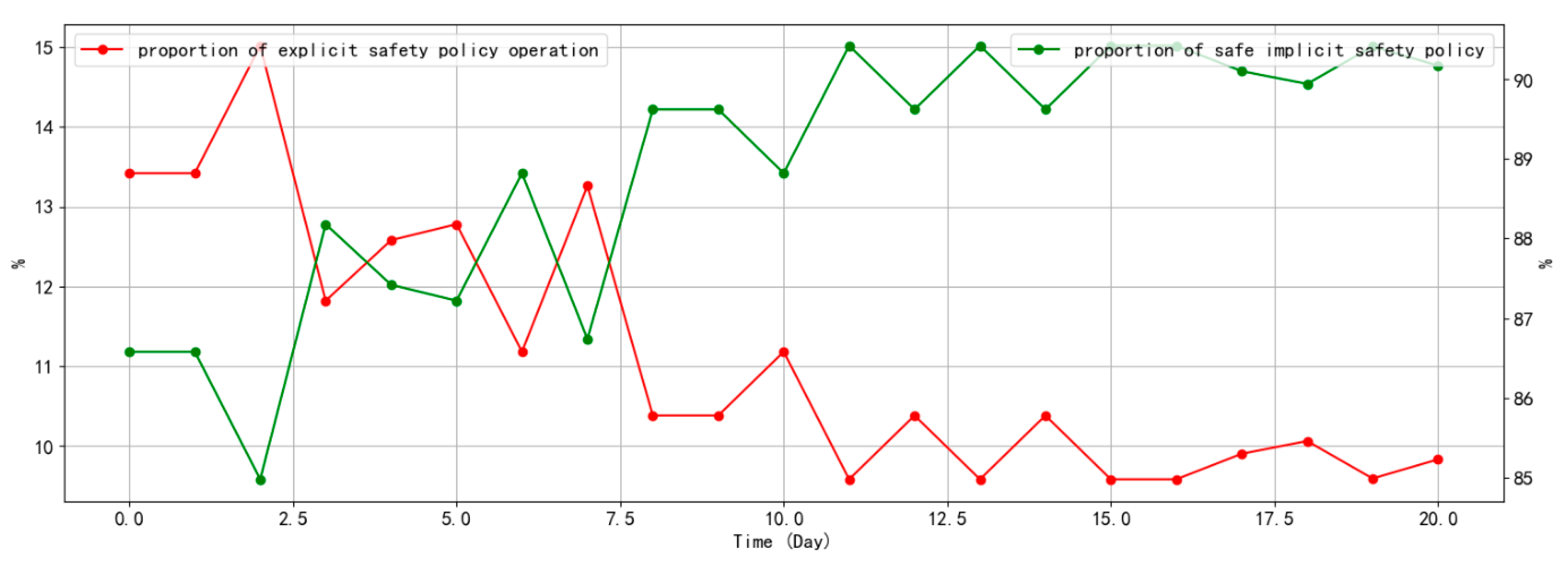
4.2.3. Performance of Safety Policies

To prevent the situation that RL cannot satisfy the thermal comfort requirements, the RL algorithm with dual safety policies for energy savings in the HVAC system is proposed. An AB test proves that the algorithm has reduced the proportion of indoor temperature dissatisfaction from 34.64% to 9.58% and decreased power consumption by 8.97%, as shown in

Table 6. Experimental Results of AB test for safety policies.

Model	Date	Average Outdoor Temperature	Average Indoor Temperature	Room TemperatureDissatisfaction Rate	Power Consumption
SAC with safety policy	17 March 2021	11.58 °C	21.06 °C	9.58%	1671.4 kWh
SAC only	18 March 2021	11.73 °C	21.37 °C	34.64%	1533.7 kWh

. Although it is difficult to compare the saving results across different HVAC systems with various algorithms due to the different system configurations and baselines, our future work will compare the results using the feasible algorithms based on a previous literature study [22]. The studies [42,43] showed two case studies with computational simulation.

The majority of indoor temperature dissatisfaction during the algorithm occurs when the system is just turned on. As can be seen from Figure 12, the heat pump outlet water temperature, primary chilled water pump frequency, and AHU water valve position are controlled to ensure the indoor temperature rises as quickly as possible when the system is just turned on. Subsequently, there will be no indoor temperature dissatisfaction. When the system is not operated under safety policies, the action is in a larger range. The indoor temperature dissatisfaction lasted for a long time after the system was turned on. Therefore, the safety policies can better safely control, thus reducing indoor temperature dissatisfaction occurrence.

On the premise that the outdoor temperature and the precision of the online safety classifier are stable, as shown in Figure 13, we counted the proportion of explicit safety policy operation of each day under the same operation hours, decreasing from 14% at the beginning to about 9.5%, which means the unsafe actions outputted by implicit safety policy decreased by 32.14%. Additionally, the proportion of outputted safe implicit safety policy increases from 85% to 90%. This indicates that the implicit safety policy could obtain a safer policy after a period of learning. However, when the device is just turned on, it is still unavoidable that the indoor temperature cannot meet the demand.

5. Conclusions

In this article, RL with dual safety policies for energy savings in an HVAC system is proposed. RL is used to solve the typical data drift issue in HVAC control systems and improve the adaptability of the control algorithm. To solve the potential unsafe risk caused by the “trial and error” attribute of RL, the dual safety policies of implicit safety policy and explicit safety policy are proposed to restrict the exploration boundary of RL. Implicit safety policy takes the safety as one of the learning objectives to improve the optimization criterion of RL. Explicit safety policy uses the data generated from the RL algorithm to learn an online safety classifier by means of online learning. For a given state, alternative action collection that meets the temperature demand is used, and a best action is selected.

To verify the effectiveness of the proposed algorithm, it is implemented in the real HVAC system of a commercial building. The result shows that the energy consumption of the building has been reduced by 15.02%, compared to traditional rule control and PID control. The proportion of room temperature dissatisfaction decreased by 25.06% compared to RL only. With the increase in the amount of data, the accuracy of the online safety classifier has not changed significantly, and remains above 90%. After a period of learning, the implicit safety policy reduces the proportion of unsafe actions by about 32.14%. Moreover, the proposed algorithm has a certain generalization ability. This proves that this control algorithm has good practicability, and can effectively reduce the energy consumption and ensure safe exploration encountered in the real HVAC system.

The future work will mainly focus on three aspects. The first aspect is to improve the convergence speed of RL. The current convergence in practical applications still takes a relatively long time, which greatly limits the algorithm verification and improvement. In future, our work will not limit the state selection, reward design, network parameter settings of RL, but also involve the combination of the prior knowledge and RL. The second is to verify the generalization capability of our algorithm in more scenarios. Due to the discrepancies of different HVAC systems, the boundaries of the generalization capability of this proposed algorithm still need to be further explored. Third, the method of simultaneous optimization of discrete and continuous actions should be introduced into the proposed control algorithm, and the method can expand the application scope of the control algorithm. In an actual scenario, both operating parameters of the system and status of equipment need to be optimized simultaneously.

References

1. Niu, Z.; Wu, J.; Liu, X.; Huang, L.; Nielsen, P.S. Understanding energy demand behaviors through spatio-temporal smart meter data analysis. Energy 2021, 226, 120493. [Google Scholar] [CrossRef]
2. Biemann, M.; Scheller, F.; Liu, X.; Huang, L. Experimental evaluation of model-free reinforcement learning algorithms for continuous HVAC control. Appl. Energy 2021, 298, 117164. [Google Scholar] [CrossRef]
3. Geng, G.; Geary, G.M. On performance and tuning of PID controllers in HVAC systems. In Proceedings of the IEEE International Conference on Control and Applications, Vancouver, BC, Canada, 13–16 September 1993; Volume 2, pp. 819–824. [Google Scholar] [CrossRef]
4. Royapoor, M.; Antony, A.; Roskilly, T. A review of building climate and plant controls, and a survey of industry perspectives. Energy Build. 2018, 158, 453–465. [Google Scholar] [CrossRef]
5. Afram, A.; Janabi-Sharifi, F. Theory and applications of HVAC control systems–A review of model predictive control (MPC). Build. Environ. 2014, 72, 343–355. [Google Scholar] [CrossRef]
6. Namatēvs, I. Deep Reinforcement Learning on HVAC Control. Inf. Technol. Manag. Sci. 2018, 21, 29–36. [Google Scholar] [CrossRef] [Green Version]
7. Wang, Z.; Hong, T. Reinforcement learning for building controls: The opportunities and challenges. Appl. Energy 2020, 269, 115036. [Google Scholar] [CrossRef]
8. Schreiber, T.; Eschweiler, S.; Baranski, M.; Dirk, M. Application of two promising Reinforcement Learning algorithms for load shifting in a cooling supply System—ScienceDirect. Energy Build. 2020, 229, 110490. [Google Scholar] [CrossRef]
9. Afroz, Z.; Shafiullah, G.M.; Urmee, T.; Higgins, G. Modeling techniques used in building HVAC control systems: A review. Renew. Sustain. Energy Rev. 2018, 83, 64–84. [Google Scholar] [CrossRef]
10. Kontes, G.D.; Giannakis, G.I.; Sánchez, V.; Agustin-Camacho, P.D.; Gruen, G. Simulation-based evaluation and optimization of control strategies in buildings. Energies 2018, 11, 3376. [Google Scholar] [CrossRef] [Green Version]
11. Azuatalam, D.; Lee, W.L.; de Nijs, F.; Liebman, A. Reinforcement learning for whole-building HVAC control and demand response. Energy AI 2020, 2, 100020. [Google Scholar] [CrossRef]
12. Raman, N.S.; Devraj, A.M.; Barooah, P.; Meyn, S.P. Reinforcement Learning for Control of Building HVAC Systems[C]//2020 American Control Conference (ACC); IEEE: New York, NY, USA, 2020; pp. 2326–2332. [Google Scholar]
13. Mason, K.; Grijalva, S. A review of reinforcement learning for autonomous building energy management. Comput. Electr. Eng. 2019, 78, 300–312. [Google Scholar] [CrossRef] [Green Version]
14. Baxter, J.; Bartlett, P.L. Infinite-horizon policy-gradient estimation. J. Artif. Intell. Res. 2001, 15, 319–350. [Google Scholar] [CrossRef]
15. Haarnoja, T.; Zhou, A.; Hartikainen, K.; Tucker, G.; Ha, S.; Tan, J.; Kumar, V.; Zhu, H.; Gupta, A.; Abbeel, P.; et al. Soft actor-critic algorithms and applications. arXiv 2018, arXiv:1812.05905. [Google Scholar]
16. Haarnoja, T.; Zhou, A.; Abbeel, P.; Levine, S. Soft actor-critic: Off-Policy maximum entropy deep reinforcement learning with a stochastic actor. In Proceedings of the 35th International Conference on Machine Learning, Stockholm, Sweden, 10–15 July 2018. [Google Scholar]
17. Zhang, C.; Kuppannagari, S.R.; Kannan, R.; Prasanna, V.K. Building HVAC scheduling using reinforcement learning via neural network based model approximation. In Proceedings of the 6th ACM International Conference on Systems for Energy-Efficient Buildings, Cities, and Transportation, New York, NY, USA, 13 November 2019; pp. 287–296. [Google Scholar]
18. Liu, Y.; Halev, A.; Liu, X. Policy learning with constraints in model-free reinforcement learning: A survey. In Proceedings of the Thirtieth International Joint Conference on Artificial Intelligence, Montreal, QC, Canada, 18 January 2021. [Google Scholar]
19. Chow, Y.; Nachum, O.; Duenez-Guzman, E.; Ghavamzadeh, M. A lyapunov-based approach to safe reinforcement learning. In Proceedings of the Advances in Neural Information Processing Systems 31 (NeurIPS 2018), Montreal, QC, Canada, 3–8 December 2018. [Google Scholar]
20. Pham, T.H.; De Magistris, G.; Tachibana, R. Optlayer-practical constrained optimization for deep reinforcement learning in the real world. In Proceedings of the 2018 IEEE International Conference on Robotics and Automation (ICRA), Brisbane, Australia, 21–25 May 2018; pp. 6236–6243. [Google Scholar]
21. Wei, T.; Wang, Y.; Zhu, Q. Deep reinforcement learning for building HVAC control. In Proceedings of the 54th Annual Design Automation Conference 2017, Austin, TX, USA, 18–22 June 2017; pp. 1–6. [Google Scholar]
22. Stavrakakis, G.M.; Katsaprakakis, D.A.; Damasiotis, M. Basic Principles, Most Common Computational Tools, and Capabilities for Building Energy and Urban Microclimate Simulations. Energies 2021, 14, 6707. [Google Scholar] [CrossRef]
23. Fu, Y.; Zuo, W.; Wetter, M.; Vangilder, J.W.; Han, X.; Plamondon, D. Equation-Based Object-Oriented Modeling and Simulation for Data Center Cooling: A Case Study. Energy Build. 2019, 186, 108–125. [Google Scholar] [CrossRef]
24. Yu, L.; Sun, Y.; Xu, Z.; Shen, C.; Yue, D.; Jiang, T.; Guan, X. Multi-agent deep reinforcement learning for HVAC control in commercial buildings. IEEE Trans. Smart Grid 2020, 12, 407–419. [Google Scholar] [CrossRef]
25. Ke, G.; Meng, Q.; Finley, T.; Wang, T.; Chen, W.; Ma, W.; Ye, Q.; Liu, T.Y. Lightgbm: A highly efficient gradient boosting decision tree. Adv. Neural Inf. Process. Syst. 2017, 30, 3146–3154. [Google Scholar]
26. Zinkevich, M. Online convex programming and generalized infinitesimal gradient ascent. In Proceedings of the 20th International Conference on Machine Learning (icml-03), Washington, DC, USA, 21–24 August 2003; pp. 928–936. [Google Scholar]
27. Cesa-Bianchi, N.; Lugosi, G. Prediction, Learning, and Games; Cambridge University Press: Cambridge, CA, USA, 2006. [Google Scholar]
28. Lobo, J.L.; Del Ser, J.; Bifet, A.; Kasabov, N. Spiking neural networks and online learning: An overview and perspectives. Neural Netw. 2020, 121, 88–100. [Google Scholar] [CrossRef]
29. Gama, J.; Sebastiao, R.; Rodrigues, P.P. On evaluating stream learning algorithms. Mach. Learn. 2013, 90, 317–346. [Google Scholar] [CrossRef] [Green Version]
30. Pérez-Sánchez, B.; Fontenla-Romero, O.; Guijarro-Berdiñas, B. A review of adaptive online learning for artificial neural networks. Artif. Intell. Rev. 2018, 49, 281–299. [Google Scholar] [CrossRef]
31. Alippi, C.; Boracchi, G.; Roveri, M. A just-in-time adaptive classification system based on the intersection of confidence intervals rule. Neural Netw. 2011, 24, 791–800. [Google Scholar] [CrossRef] [PubMed]
32. Kuncheva, L.I.; Žliobaitė, I. On the window size for classification in changing environments. Intell. Data Anal. 2009, 13, 861–872. [Google Scholar] [CrossRef] [Green Version]
33. Ghazikhani, A.; Monsefi, R.; Yazdi, H.S. Online neural network model for non-stationary and imbalanced data stream classification. Int. J. Mach. Learn. Cybern. 2014, 5, 51–62. [Google Scholar] [CrossRef]
34. Pavlidis, N.G.; Tasoulis, D.K.; Adams, N.M.; Hand, D.J. λ-Perceptron: An adaptive classifier for data streams. Pattern Recognit. 2011, 44, 78–96. [Google Scholar] [CrossRef] [Green Version]
35. Ditzler, G.; Rosen, G.; Polikar, R. Domain adaptation bounds for multiple expert systems under concept drift. In 2014 International Joint Conference on Neural Networks (IJCNN); IEEE: Piscataway, NJ, USA, 2014; pp. 595–601. [Google Scholar]
36. Qiao, J.; Li, F.; Han, H.; Li, W. Constructive algorithm for fully connected cascade feedforward neural networks. Neurocomputing 2016, 182, 154–164. [Google Scholar] [CrossRef]
37. Thomas, P.; Suhner, M.C. A new multilayer perceptron pruning algorithm for classification and regression applications. Neural Process. Lett. 2015, 42, 437–458. [Google Scholar] [CrossRef]
38. Silva, A.M.; Caminhas, W.; Lemos, A.; Gomide, F. A fast learning algorithm for evolving neo-fuzzy neuron. Appl. Soft Comput. 2014, 14, 194–209. [Google Scholar] [CrossRef]
39. Zhang, J.; Yan, J.; Infield, D.; Liu, Y.; Lien, F.-S. Short-term forecasting and uncertainty analysis of wind turbine power based on long short-term memory network and Gaussian mixture model. Appl. Energy 2019, 241, 229–244. [Google Scholar] [CrossRef] [Green Version]
40. Qiu, D.; Dong, Z.; Zhang, X.; Wang, Y.; Strbac, G. Safe reinforcement learning for real-time automatic control in a smart energy-hub. Appl. Energy 2022, 309, 118403. [Google Scholar] [CrossRef]
41. Hochreiter, S.; Schmidhuber, J. Long Short-Term Memory. Neural Comput. 1997, 9, 1735–1780. [Google Scholar] [CrossRef]
42. Katsaprakakis, D.; Kagiamis, V.; Zidianakis, G.; Ambrosini, L. Operation Algorithms and Computational Simulation of Physical Cooling and Heat Recovery for Indoor Space Conditioning. A Case Study for a Hydro Power Plant in Lugano, Switzerland. Sustainability 2019, 11, 4574. [Google Scholar] [CrossRef] [Green Version]
43. Katsaprakakis, D.A. Computational Simulation and Dimensioning of Solar-Combi Systems for Large-Size Sports Facilities: A Case Study for the Pancretan Stadium, Crete, Greece. Energies 2020, 13, 2285. [Google Scholar] [CrossRef]
Figure 1. The schematic map of RL (the solid lines represent that the state, action and reward are generated from current timestep t , the dotted line of s t + 1 is obtained from the next timestep t + 1 ).
Buildings 13 00580 g001
Figure 2. Schematic diagram of the corresponding relationship between the consumed power and the indoor demand satisfaction.
Buildings 13 00580 g002
Figure 3. Schematic diagram of RL with dual safety policies.
Buildings 13 00580 g003
Figure 4. The network of the online safety classifier based on residual learning.
Buildings 13 00580 g004
Figure 5. The main structure of LSTM.
Buildings 13 00580 g005
Figure 6. HVAC system schematic diagram.
Buildings 13 00580 g006
Figure 7. Reward trend of reinforcement learning.
Buildings 13 00580 g007
Figure 8. Power consumption and indoor temperature penalty trends of proposed RL algorithm.
Buildings 13 00580 g008
Figure 9. Temperature indoor and outdoor trends of AB tests (the grey area represents the AI_status is 0, the red area represents the AI_status is 1).
Buildings 13 00580 g009
Figure 10. Power trends of AB tests (the grey area represents the AI_status is 0, the red area represents the AI_status is 1).
Buildings 13 00580 g010
Figure 11. Action trends of AB tests (the grey area represents the AI_status is 0, the red area represents the AI_status is 1).
Buildings 13 00580 g011
Figure 12. AB test action trends by safety policies.
Buildings 13 00580 g012
Figure 13. The proportion of explicit safety policy operation and safe implicit safety policy.
Buildings 13 00580 g013