A Fast Method for Calculating the Impact of Occupancy on Commercial Building Energy Consumption

Abstract

Occupancy, which refers to the occupant count in this paper, is one of the main factors affecting the energy consumption of commercial buildings. It is important for both building managers and energy simulation engineers to understand how an entire building’s energy consumption varies with different occupancy levels in the process of building automation systems or in assessments of building performance with benchmarking lines. Because commercial buildings usually have large scales, complex layouts and a large number of people, it is a challenge to simulate the relationships between an entire building’s energy consumption and occupancy. This study proposes a fast method for calculating the influence of occupancy on the energy consumption of commercial buildings with different building layouts and existing occupancies. Other occupant behaviors, such as the opening of windows and adjustment of shading devices, are comprehensively reflected in two basic building parameters: the balance point temperature and the total heat transmission coefficient of the building. This new method can be easily used to analyze how building energy varies with occupancy without a physical building’s energy model. An office building in Shanghai is taken as a case study to validate the proposed method. The results show that the coefficient of determination R² between the calculated value and actual value is 0.86, 0.8 and 0.71 for lighting, cooling and heating energy, respectively, which is suitable in engineering applications.

1. Introduction

Globally, building energy is an important sector of energy consumption. According to International Energy Outlook 2021 [1], the global energy consumption of buildings is expected to increase from 2020 to 2050, especially for countries not affiliated with the Organization for Economic Cooperation and Development (non-OECD). In 2050, the building sector will account for more than half of non-OECD electricity use. In China, the commercial building sector (excluding the energy for heating in North China) accounted for 33% of the total building energy consumption in 2020. The energy use intensity (EUI) of commercial buildings increased from 17 kgce/m² in 2001 to 24.7 kgce/m² in 2020. New construction of commercial buildings, particularly large-scale buildings, and the increasing need for building services has led to a rapid increase in energy consumption [2].

Occupant behaviors, including occupant presence and their interactions with building systems, influence building energy consumption both directly and indirectly [3]. The impacts of occupants on the building energy consumption can be divided into three categories: the utilization of lighting and electrical appliances; elevators and escalators; and heating, ventilation and air-conditioning (HVAC) systems. Figure 1 shows a flowchart of how occupants affect building energy consumption in detail. Occupants may use numerous lighting and electrical appliances in the building, contributing to electricity consumption directly and to internal loads that lead to HVAC consumption indirectly. Occupancy also contributes to internal loads. In addition, in consideration of the occupants’ health, an adequate volume of fresh air is required to meet the ventilation needs of the occupants. Some occupant behaviors change the parameters of the HVAC system to enhance personal comfort. For example, occupants can set the temperature and humidity of rooms. Their interactions with windows and shading devices such as blinds and curtains change the infiltration rate and shading coefficients, respectively. Moreover, occupant movement between different floors in buildings generates elevator and escalator energy consumption.

To gain insight into the relationship between occupant behaviors and building energy consumption, the International Energy Agency (IEA) established Annex 66 [4] and Annex 79 [5] to develop occupant behavior models and apply them to building design and control. Various static models, stochastic models and machine learning models have been used to simulate the presence of occupants and other behaviors, which are summarized in

Table 1. Summary of occupant behavior models.

Occupant Behavior	Modeling Approach	Reference
Presence	Markov chain	[6,7]
	Pattern (clustering)	[8,9]
Lighting on/off	Pattern	[10]
	Markov chain	[11]
	Probabilistic formula	[12]
	Poisson process	[13]
The use of appliances	Monte Carlo	[14]
	Logistic regression	[15]
Thermostat control	Markov chain	[16]
	Logistic regression	[15,16]
Open/close windows	Markov chain	[17]
	Logistic regression	[15,17]
	Agent-based	[18]
Shading control	Logistic regression	[15,19]

.

Among these occupant-related factors, occupancy is the most essential in determining commercial building energy consumption [20]. One reason for this is that occupancy is considered the basis of occupant behavior. The other reason is that for most current commercial buildings, building automation (BA) systems are usually centrally controlled by facility managers, so occupant intervention is quite limited. In building control, building facility managers need to know how building energy varies with occupancy in order to change the operation status of the equipment in the BA system. Zou et al. [21] implemented an occupancy-driven lighting control system in an office building in Singapore, achieving 93.09% lighting energy savings compared to static scheduling lighting control scheme. Tekler et al. [22] proposed an IoT-based, occupancy-driven smart plug load management system and the best occupancy-driven control strategy achieved a 7.5% reduction in building energy consumption. Extant research [23,24,25,26,27] has shown that commercial buildings could save 9–42% building energy when using occupancy-based HVAC control. For building energy assessments, it is necessary to eliminate the impact of both occupancy and weather in order to evaluate the actual building performance. Therefore, it is worth studying occupancy’s impact on commercial building energy consumption.

In order to study the relationship between occupancy and building energy consumption, much research has focused on how to obtain occupancy data in building. These measurement methods could be grouped into questionnaire survey method and monitoring method [28]. The questionnaire survey method saves the cost of installing sensors and protects occupant privacy, but it needs a large amount of work in terms of data analysis. Thus, questionnaires are usually used to collect occupancy data in residential buildings [28]. Occupancy data can be directly or indirectly detected using different monitoring tools, such as passive infrared (PIR) sensor, camera, CO₂ sensor, Bluetooth, Wi-Fi and so on. Floyd et al. [29] detected occupancy data using PIR sensors and applied occupancy data to lighting control. Benezeth et al. [30] obtained occupant information, including location, count, activity, identity and track, using video cameras. Wang et al. [31] demonstrated an occupancy-based ventilation control system by estimating occupancy with CO₂ concentration data. Vafeiadis et al. [32] estimated occupancy by data gathered from electricity and water consumption smart meters. Tekler and Chong [33] estimated occupancy with different sensor data, including indoor environmental and outdoor weather condition data, number of Wi-Fi-connected devices, energy consumption data, HVAC operations, and time-related information. In recent years, with the development of Internet and communication technology, it is convenient to use mobile devices such as smartphones to track occupant movement and detect occupancy in buildings. Depatla et al. [34] estimated occupancy with Wi-Fi power measurements. Tekler et al. [35] estimated occupancy at zone level with Bluetooth-low-energy (BLE) technology in smartphone devices. Lu et al. [36] extracted occupancy patterns from social media, including Twitter, Facebook and Google Map. Compared with other monitoring methods, the mobile device detection method is cheap and convenient. It is suitable for all kinds of buildings, especially for large-scale buildings.

Previous research about occupancy’s impact on building energy can be classified into three groups. (1) The first uses building performance simulation (BPS) tools. Hong et al. [37] developed an occupant behavior functional mock-up unit (obFMU) to co-simulate building energy with BPS tools, such as EnergyPlus or DeST. Jia [38] used an agent-based model and EnergyPlus to simulate occupant-related energy consumption. This method takes the stochastic nature of occupant behavior into consideration and can be applied to both residential and commercial buildings. However, this method needs a physical building model in BPS tools, and the simulation speed is related to the scale of the building model. Thus, for buildings with large scales, complex layouts and a large number of occupants, this method costs much more labor and time. (2) The second research group uses data-driven building energy simulation models to analyze the impact of occupant behavior. The models are developed based on large amounts of data, including building information, weather data and occupant-related data, collected using simulation or from the real world. Sha et al. [39] developed a key-variable-based parallel model to predict HVAC energy. In this study, occupant-related variables comprised occupancy density, lighting power density, heating and cooling setpoint temperatures, infiltration rate and interior shading rate. Amasyali and El-Gohary [40] used EnergyPlus to generate training dataset and developed a set of machine learning-based cooling energy prediction models. The results showed that cooling setpoint and window operation were the most influential occupant-related variables. They also proposed a real data-driven method to assess the energy saving potential of occupant behavior improvements considering occupant comfort [41]. Compared to BPS tools, data-driven methods usually need fewer input variables and are more convenient to train. However, this kind of method has two limitations. Firstly, data-driven models usually have poor performance when the training data and test data are drawn from different feature spaces or different distributions. Secondly, for buildings without historical data, BPS tools are still needed to generate training data. (3) The third research group is uses constant influence intensity, i.e., energy per occupant. The Pacific Northwest National Laboratory (PNNL) proposed a full-time equivalent occupancy (FTEO)-adjusted energy use intensity metric to estimate the EUI at the FTEO level, which is the ratio of total occupancy hours to full-time equivalent hours [42]. Kim and Srebric [43] used a linear regression model to calculate the electric energy rate per occupant based on areas with different functions. This method calculates occupancy’s influence using the products of influence intensity and occupancy. This method is very easy and convenient to use. However, the influence intensity is constant and building energy consumption is assumed to increase with occupancy or equivalent occupancy, but the influence intensity actually varies with the occupancy and usually exhibits a decreasing trend, as shown in Figure 2. This is because the occupancy’s influence on building energy is related to the existing occupancy. When there are only a few people in the building, new people arriving turn on lights and generate extra lighting energy consumption. When the existing occupancy increases to a certain level and all the BA systems’ equipment is at full operational load, the new arriving people do not generate extra energy consumption, and the energy per occupant decreases.

In addition to the existing occupancy, the occupancy’s impact on energy consumption is also associated with building automation level. The impact of occupancy and occupant behaviors on building energy is limited for fully automated controlled buildings, as shown in Figure 2. In commercial buildings, the lighting and HVAC equipment in public spaces is usually controlled by building facility managers, while single- or multi-person rooms are manually controlled by the occupants. The higher the proportion of public spaces in the building, the higher the building automation level. Thus, for commercial buildings, the building layout could represent the building automation level indirectly.

This study proposes a fast method for calculating the occupancy’s impact on commercial building energy consumption at the whole building level. The main innovations of the proposed method include (1) the building layout and existing occupancy being taken into consideration, which have generally been ignored in previous studies; (2) other occupant behaviors are simplified into two basic building parameters, the balance point temperature and the total heat transmission coefficient of the building; and (3) this method does not require a physical building energy model, so it is fast and convenient to calculate the occupancy’s influence on commercial energy consumption in different scenarios.

In this paper, the proposed method is used to analyze the influence of occupancy on building energy consumption at different existing occupancy levels for different building layouts. A sensitivity analysis is conducted to discuss the key factors affecting occupancy’s influence. Finally, the proposed method is applied in an office building in Shanghai as a case study. The rest of this paper is organized as follows. The occupancy’s influence calculation method, the sensitivity analysis method and case study information are introduced in Section 2. The calculation results of proposed model in different scenarios, the sensitivity results and case study results are shown in Section 3. The performance of the proposed method is discussed in Section 4. The advantages and limitations of the proposed method and recommendations for future work are concluded in Section 5.

2. Methodology

2.1. Method for Calculating the Occupancy’s Influence

As shown in Figure 1, the impact of occupancy on building energy consumption can be classified into three major parts: lighting and electrical appliances, the HVAC system and elevators and escalators. Because the elevators and escalators sector only accounts for 3–5% of total building energy [44], the method in this study mainly focuses on the occupancy’s impact on the energy consumption from lighting, electrical appliances and HVAC, as shown in Equation (1):

∆E_total = ∆E_light + ∆E_equip + ∆E_hvac,

(1)

where ∆E_total is the total energy consumption change when occupancy changes, and ∆E_light, ∆E_equip and ∆E_hvac represent the change in the energy consumption of the lighting, electrical appliances and HVAC, respectively.

The key parameters and equations used in proposed method are shown in Figure 3. Parameters in yellow boxes and orange boxes reflect the building layout information and parameters related to occupant behaviors, respectively. The balance point temperature represents occupants’ interactions with thermostats. Other occupant behaviors, such as opening windows and adjusting shading devices, are comprehensively reflected in the total heat transmission coefficient of the building.

2.1.1. Lighting Energy Consumption

The lighting energy consumption in commercial buildings can be divided into public lighting, plug lighting and switch lighting. Public lighting, such as the lighting in entrance halls and corridors, emergency lighting and flood lighting, is usually controlled by the facility managers and does not change with the building occupancy. Plug lighting, which is produced by personal auxiliary lighting equipment, such as table lamps, is generated only when the switch lighting in the space cannot provide sufficient illumination for occupants. Thus, it accounts for a small proportion of the lighting energy in current commercial buildings. Switch lighting is the lighting energy consumption produced when occupants enter a room or a space and turn on the light switch. This contributes the most to commercial buildings’ lighting energy consumption when occupancy varies. It is also related to the existing occupancy and the building layout.

The building layout has a direct impact on the marginal energy consumption caused by extra occupants. Figure 4 illustrates two different building layouts. There are 10 single-person rooms in layout (a) and 2 five-person rooms in layout (b). The total area and the lighting density are the same in both cases. Occupants turn on the lights when they enter a room. If there is one occupant in the building and one new person enters, the lighting energy consumption increases by one unit in (a). However, in case (b), there is a 50% chance that the lighting energy consumption will increase and a 50% chance that the lighting energy consumption will remain the same with the entry of one new occupant; the average effect is thus 2.5 units. However, if there are six occupants in the building and one additional person enters, the lighting energy consumption again increases by one unit in (a) but does not change in (b). Therefore, the effect of occupancy on switch lighting can be written as Equation (2):

$$\mathsf{\Delta }{\mathrm{E}}_{\mathrm{switch} }=\sum {\mathrm{P}}_{\mathrm{enter}|\mathrm{totalN}·\mathrm{baseN}·\mathrm{roomN}·\mathsf{\Delta }\mathrm{N}}{\mathrm{A}}_{\mathrm{switch}}{\mathsf{\rho }}_{\mathrm{switch}}{\mathrm{M}}_{\mathrm{onoff}},$$

(2)

where $\mathrm{totalN}$ is the total maximum occupancy of nonpublic rooms and spaces in the building; $\mathrm{baseN}$ is the existing occupancy in the building; $\mathsf{\Delta }\mathrm{N}$ is the number of added occupants; $\mathrm{roomN}$ is the nominal occupancy of each room in the building (1 for single rooms, 2 for two-person rooms, etc.); ${\mathrm{A}}_{\mathrm{switch}}$ is the total area of each type of room (m²); ${\mathsf{\rho }}_{\mathrm{switch}}$ is the switch lighting power density (W/m²); and ${\mathrm{M}}_{\mathrm{onoff}}$ is the lighting control strategy, which can be set as one if the light is turned on when occupant enters the room. If the occupants control the lighting equipment according to the illumination level, this value can be set by referring to the probability curve in [10,11,12]; ${\mathrm{P}}_{\mathrm{enter}|\mathrm{totalN}·\mathrm{baseN}·\mathrm{roomN}·\mathsf{\Delta }\mathrm{N}}$ represents the probability that $\mathsf{\Delta }\mathrm{N}$ occupants enter a $\mathrm{roomN}$-type room with $\mathrm{baseN}$ existing occupants in the building, which can be calculated using Equation (3):

$${\mathrm{P}}_{\mathrm{enter}|\mathrm{totalN}·\mathrm{baseN}·\mathrm{roomN}·\mathsf{\Delta }\mathrm{N}}=\left\{\begin{array}{c}{\mathrm{P}}_1·\left({1 - \mathrm{P}}_2\right), 0 < \mathsf{\Delta }\mathrm{N} < \mathrm{b}\hfill \\ {\mathrm{P}}_1 , \mathsf{\Delta }\mathrm{N} \ge \mathrm{b} > 0\hfill \\ 0 , \mathrm{b} \le 0 \hfill \end{array}\right.,$$

(3)

where ${\mathrm{P}}_1$ represents the probability that none of the existing $\mathrm{baseN}$ occupants are in a $\mathrm{roomN}$-type room, which can be calculated by Equation (4); ${\mathrm{P}}_2$ represents the probability that no $\mathsf{\Delta }\mathrm{N}$ new occupants entering a $\mathrm{roomN}$-type room, which can be calculated by Equation (5). Thus, 1 − ${\mathrm{P}}_2$ represents the probability of $\mathsf{\Delta }\mathrm{N}$ new occupants entering a $\mathrm{roomN}$-type room: b = $\mathrm{totalN} - \mathrm{baseN} - \mathrm{roomN}$. When $\mathsf{\Delta }\mathrm{N} > \mathrm{b}$, the new arriving occupants would no longer generate more switch lighting energy for a $\mathrm{roomN}$-type room. When b ≤ 0, the $\mathrm{roomN}$-type rooms are occupied by the existing occupancy, and new occupants do not need to turn on the light. Thus, ${\mathrm{P}}_{\mathrm{enter}|\mathrm{totalN}·\mathrm{baseN}·\mathrm{roomN}·\mathsf{\Delta }\mathrm{N}}$ is 0.

$${\mathrm{P}}_1=\frac{{\mathrm{C}}_{\mathrm{totalN}-\mathrm{roomN}}^{\mathrm{baseN}}}{{\mathrm{C}}_{\mathrm{totalN}}^{\mathrm{baseN}}}={\left(\frac{\mathrm{a}·\mathrm{d}}{\mathrm{b}·\mathrm{totalN}}\right)}^{\mathrm{totalN}+0.5}{\left(\frac{\mathrm{b}}{\mathrm{a}}\right)}^{\mathrm{baseN}}{\left(\frac{\mathrm{b}}{\mathrm{d}}\right)}^{\mathrm{roomN}}$$

(4)

$${\mathrm{P}}_2=\frac{{\mathrm{C}}_{\mathrm{totalN}-\mathrm{baseN}-\mathrm{roomN}}^{\mathsf{\Delta }\mathrm{N}}}{{\mathrm{C}}_{\mathrm{totalN}-\mathrm{baseN}}^{\mathsf{\Delta }\mathrm{N}}}=\frac{\mathrm{c}{\left(\mathrm{a} - \mathsf{\Delta }\mathrm{N}\right)}^{\mathrm{a}+0.5-\mathsf{\Delta }\mathrm{N}}}{{\left(\mathrm{b} - \mathsf{\Delta }\mathrm{N}\right)}^{\mathrm{b}+0.5-\mathsf{\Delta }\mathrm{N}}}$$

(5)

$$\mathrm{n}!=\sqrt{2\mathsf{\pi }\mathrm{n}}{\left(\frac{\mathrm{n}}{\mathrm{e}}\right)}^{\mathrm{n}}$$

(6)

where $\mathrm{a}=\mathrm{totalN} - \mathrm{baseN}$; $\mathrm{c}=\frac{{\mathrm{b}}^{\mathrm{b}+0.5}}{{\mathrm{a}}^{\mathrm{a}+0.5}}$; $\mathrm{d}=\mathrm{totalN} - \mathrm{roomN}$; $\mathrm{e}$ is the natural logarithm; and ${\mathrm{C}}_{\mathrm{n}}^{\mathrm{m}}=\frac{\mathrm{n}!}{\mathrm{m}!\left(\mathrm{n}-\mathrm{m}\right)!}$ is the expression for the total number of all cases when m items are chosen from n items without return. When m and n are large, the factorial operation overflows in computers. Thus, the factorial operation is simplified using Stirling’s formula, as shown in Equation (6).

The energy consumption of plug lighting can also be calculated with Equation (2). However, there is no visible boundary in this case, and thus $\mathrm{roomN}$ represents the number of working stations where the public lighting and switch lighting cannot provide sufficient illumination.

2.1.2. Electrical Appliances Energy Consumption

The electrical appliances in commercial buildings include both public equipment and personal equipment. The energy consumption of public equipment does not change with occupancy, and the consumption of personal equipment is usually considered as plug energy consumption, which exhibits a linear relationship with occupancy in [45]. Thus,

$$\mathsf{\Delta }{\mathrm{E}}_{\mathrm{equip}}=\mathsf{\Delta }{\mathrm{E}}_{\mathrm{plugequip}}{=\mathsf{\rho }}_{\mathrm{equip}}\mathsf{\Delta }\mathrm{N},$$

(7)

where ${\mathsf{\rho }}_{\mathrm{equip}}$ represents the equipment power density (W/person).

2.1.3. HVAC Energy Consumption

In ASHARE standard [46], degree-day methods are simple and effective methods for energy analysis based on the balance point temperature ${\mathrm{T}}_{\mathrm{bal}}$, at which neither heating nor cooling is required in the building. If the outdoor air temperature is higher than ${\mathrm{T}}_{\mathrm{bal}}$, cooling is required; otherwise, heating is required. ${\mathrm{T}}_{\mathrm{bal}}$ can be calculated using Equation (8):

$${\mathrm{T}}_{\mathrm{bal}}{=\mathrm{T}}_{\mathrm{in}} - \frac{{\mathrm{q}}_{\mathrm{gain}}}{{\mathrm{K}}_{\mathrm{tot}}},$$

(8)

where ${\mathrm{T}}_{\mathrm{in}}$ is indoor air temperature (°C); ${\mathrm{q}}_{\mathrm{gain}}$ is the total heat gain from sun and internal loads (W). The heat gain from sunlight is independent of occupancy, while the occupancy would influence internal loads directly; ${\mathrm{K}}_{\mathrm{tot}}$ is the total heat transfer coefficient of the building (W/K). In ASHARE standard, ${\mathrm{K}}_{\mathrm{tot}}$ represents the heat transmission coefficient of the building with windows closed. However, in this paper, ${\mathrm{K}}_{\mathrm{tot}}$ is the total heat transmission coefficient of the building considering the effect of shading, infiltration and ventilation, which can be calculated using Equation (9) [47]:

$${\mathrm{K}}_{\mathrm{tot}}{=\mathrm{U}}_{\mathrm{tot}}{\mathrm{A}}_{\mathrm{tot}}{+\mathrm{c}}_{\mathrm{p}}{\mathrm{VN}}_{\mathrm{air}},$$

(9)

where ${\mathrm{U}}_{\mathrm{tot}}$ is the total average U-value of the building envelope (W/(Km²)); ${\mathrm{A}}_{\mathrm{tot}}$ is the total envelope area (m²); ${\mathrm{c}}_{\mathrm{p}}$ is the heat capacity of air, about 0.33(Wh)/(m³K); $\mathrm{V}$ is the enclosed volume (m³); and ${\mathrm{N}}_{\mathrm{air}}$ is the number of air changes, including ventilation and infiltration (h⁻¹).

For most current commercial buildings, the fresh air volume is constant during operation. Thus, ${\mathrm{K}}_{\mathrm{tot}}$ would not change with occupancy. If the fresh air volume is changed with occupancy by 30 m³/h per occupant, ${\mathrm{K}}_{\mathrm{tot}}$ would change to

$${\mathrm{K}}_{\mathrm{tot}}^{\prime }{=\mathrm{U}}_{\mathrm{tot}}{\mathrm{A}}_{\mathrm{tot}}{+\mathrm{c}}_{\mathrm{p}}\mathrm{V}\left({\mathrm{N}}_{\mathrm{air}}+\frac{30\mathsf{\Delta }\mathrm{N}}{\mathrm{V}}\right){=\mathrm{K}}_{\mathrm{tot}}+9.9\mathsf{\Delta }\mathrm{N}.$$

(10)

Therefore, occupancy mainly influences the HVAC energy consumption by changing ${\mathrm{T}}_{\mathrm{bal}}$ and ${\mathrm{K}}_{\mathrm{tot}}$. Thermostat control changes ${\mathrm{T}}_{\mathrm{in}}$. Opening/closing windows changes the ${\mathrm{N}}_{\mathrm{air}}$. Shading control would change ${\mathrm{U}}_{\mathrm{tot}}$, and then change ${\mathrm{K}}_{\mathrm{tot}}$. Because the energy consumption change of fresh air fans is too small compared to that of source equipment, such as chillers and boilers, the energy consumption change of fresh air fans is ignored in this paper. Occupancy impact on the HVAC energy consumption can be calculated using Equations (11) and (12):

$$\mathsf{\Delta }{\mathrm{Q}}_{\mathrm{hvac}}{=\mathrm{K}}_{\mathrm{tot},\mathrm{h}}^{\prime }{\left[{\mathrm{T}}_{\mathrm{bal},\mathrm{h}}^{\prime }{ - \mathrm{T}}_{\mathrm{out}}\right]}^{+}{ - \mathrm{K}}_{\mathrm{tot},\mathrm{h}}{\left[{\mathrm{T}}_{\mathrm{bal},\mathrm{h}}{ - \mathrm{T}}_{\mathrm{out}}\right]}^{+}{+\mathrm{K}}_{\mathrm{tot},\mathrm{c}}^{\prime }{\left[{\mathrm{T}}_{\mathrm{out}}{ - \mathrm{T}}_{\mathrm{bal},\mathrm{c}}^{\prime }\right]}^{+}{ - \mathrm{K}}_{\mathrm{tot},\mathrm{c}}{\left[{\mathrm{T}}_{\mathrm{out}}{ - \mathrm{T}}_{\mathrm{bal},\mathrm{c}}\right]}^{+},$$

(11)

$$\mathsf{\Delta }{\mathrm{E}}_{\mathrm{hvac} }=\frac{\mathsf{\Delta }{\mathrm{Q}}_{\mathrm{hvac}}}{\mathrm{COP}},$$

(12)

where the plus sign above the bracket in Equation (11) indicates that only positive values are counted; the subscript c and h represent cooling and heating conditions, respectively; $\mathsf{\Delta }{\mathrm{Q}}_{\mathrm{hvac}}$ is the change in HVAC loads (W); $\mathsf{\Delta }{\mathrm{E}}_{\mathrm{hvac}}$ is the change in HVAC energy consumption (W); ${\mathrm{T}}_{\mathrm{out}}$ is the outdoor air temperature (°C); COP is the coefficient of performance of HVAC system; and ${\mathrm{T}}_{\mathrm{bal}}^{\prime }$ represents the balance point temperature after occupancy change (°C). As ${\mathrm{q}}_{\mathrm{gain}}$ changes when the occupancy is much larger than ${\mathrm{K}}_{\mathrm{tot}}$, ${\mathrm{T}}_{\mathrm{bal}}^{\prime }$ is simplified as:

$${\mathrm{T}}_{\mathrm{bal}}^{\prime }{=\mathrm{T}}_{\mathrm{in}} - \frac{{\mathrm{q}}_{\mathrm{gain}}{+\mathsf{\Delta }\mathrm{Q}}_{\mathrm{inter},\mathrm{sensible}}}{{\mathrm{K}}_{\mathrm{tot}}^{\prime }} \approx { \mathrm{T}}_{\mathrm{in}} - \frac{{\mathrm{q}}_{\mathrm{gain}}}{{\mathrm{K}}_{\mathrm{tot}}} - \frac{{\mathsf{\Delta }\mathrm{Q}}_{\mathrm{inter},\mathrm{sensible}}}{{\mathrm{K}}_{\mathrm{tot}}^{\prime }}{=\mathrm{T}}_{\mathrm{bal}} - \frac{{\mathsf{\Delta }\mathrm{Q}}_{\mathrm{inter},\mathrm{sensible}}}{{\mathrm{K}}_{\mathrm{tot}}^{\prime }} ,$$

(13)

$${\mathsf{\Delta }\mathrm{Q}}_{\mathrm{inter},\mathrm{sensible}}{=\mathrm{CL}}_{\mathrm{light}}{\mathsf{\Delta }\mathrm{E}}_{\mathrm{light}}{+\mathrm{CL}}_{\mathrm{equip}}{\mathsf{\Delta }\mathrm{E}}_{\mathrm{equip}}{+\mathrm{CL}}_{\mathrm{occ}}{\mathsf{\Delta }\mathrm{Q}}_{\mathrm{occ}},$$

(14)

$$\mathsf{\Delta }{\mathrm{Q}}_{\mathrm{occ}}{=\mathrm{qn}}^{\prime }\mathsf{\Delta }\mathrm{N} ,$$

(15)

where ${\mathsf{\Delta }\mathrm{Q}}_{\mathrm{inter},\mathrm{sensible}}$ is the change in the sensible internal heat load (W); ${\mathrm{CL}}_{\mathrm{light}}$, ${\mathrm{CL}}_{\mathrm{equip}}$ and ${\mathrm{CL}}_{\mathrm{occ}}$ represent the cooling load coefficients of lighting equipment and occupants, respectively; $\mathsf{\Delta }$Q_occ is the change in the occupant load (W); q is the sensible heat of each occupant, W/person; ${\mathrm{n}}^{,}$ is the clustering coefficient of occupants; ${\mathsf{\Delta }\mathrm{E}}_{\mathrm{light}}$ and ${\mathsf{\Delta }\mathrm{E}}_{\mathrm{equip}}$ represent the energy consumption change in the light and electrical appliances sectors, respectively.

In this paper, the proposed method is used to analyze the influence of occupancy on building energy consumption at different existing occupancy levels for different building layouts. The basic input parameters used in analysis are listed in

Table 2. Basic input parameters used in analysis.

Energy/Load	Input Parameters
Lighting	roomN = [1, 2, 4, 6, 100], Aswitch = [720, 800, 800, 1000, 3000] m2, totalN = 1160, ρswitch = 10 W/m2, Monoff = 1, ∆Epluglight = 0
Electrical appliances	ρequip =160 W/person
Occupancy	q = 100 W/person, n’ = 0.9
HVAC	CLlight = 0.41, CLequip = 0.56, CLocc = 0.51, COP = 3.5, Ktot,h = Ktot,c = 35,000 W/K, Tbal,h = 18 °C, Tbal,c = 24 °C

. It assumed that the building contains twenty single rooms, twenty 2-person rooms, ten 4-person rooms, ten 6-person rooms and ten 100-person rooms. Thus, totalN is 1160. And the total area of each type rooms are 720 m², 800 m², 800 m², 1000 m² and 3000 m², respectively. M_onoff is assumed to be 1 and ∆E_pluglight to be 0. CL_light, CL_equip and CL_occ are chosen from the Appendix in [48]. Other input parameters are settled based on empirical data in Shanghai.

2.2. Sensitivity Analysis Method of Model Inputs

A sensitivity analysis was used to determine the impact of occupant-related parameters. Because the number of inputs in this method was fairly small, the Sobol method was applied to analyze the influence of the main inputs on the energy consumption change. The Sobol method is a model-free global sensitivity analysis method that can be used for both linear and nonlinear models [49]. It can provide sensitivity indices for the first-order effects, which comprise the main effects on the output variations due to the corresponding input. This method can also provide the total effect factor, which accounts for the total contribution to the output variance due to the corresponding input; this includes both first-order and higher-order effects owing to the interactions among inputs. Because this method estimates the sensitivity indices using the Monte Carlo approach, quasi-random number generators, such as the Sobol sequence, outperform Monte Carlo sampling for the estimation of multidimensional integrals. In this study, the SALib package [50] in Python was used for Sobol analysis. The sampling method is Saltelli’s extension of the Sobol sequence. The inputs and their bounds are listed in

Table 3. Bounds of inputs in sensitivity analysis.

Input	Note	Unit	Nomenclature in Figure	Bounds
$\mathsf{\Delta }$N	Number of added occupants	person	$\mathsf{\Delta }$N	[0, 1000]
baseN	Existing occupancy in the building	person	baseN	[0, 1000]
ρlight	Power density of lighting	W/m2	Power_light	[11, 60]
ρequip	Power density of equipment	W/person	Power_equip	[40, 100]
Ktot,h	Total heat transmission coefficient of the building in heating season	W/K	Ktoth	[4000, 40,000]
Ktot,c	Total heat transmission coefficient of the building in cooling season	W/K	Ktotc	[4000, 40,000]
Tbal,h	B Balance point temperature in heating season	°C	Tbh	[14, 18]
Tbal,c	Balance point temperature in cooling season	°C	Tbc	[20, 24]
Tout	Outdoor air temperature	°C	Tout	[−10, 37]
COP	Coefficient of performance	W/W	COP	[2, 5]

.

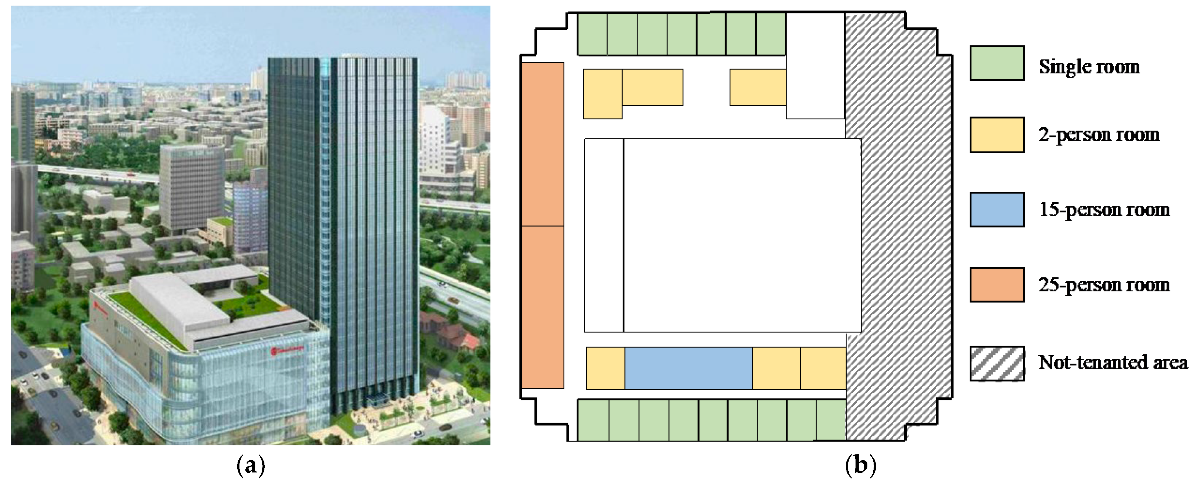
2.3. Case Study Information

A 35-storey office building with CAV and VAV systems in Shanghai was chosen as a case study. The building is 132 m high, covering an area of 92,688.4 m² on the ground. The four underground floors are parking garages and a civil air defense area. The first and second floors are office halls, and the above areas are office areas. Approximately 40% of the area, including office spaces and public area, such as elevators, corridors and toilets, have been tenanted. Figure 5 shows the building photo and the layout of one floor. The white area in Figure 5b is public space. The proposed method was applied to calculate the ∆E_light and ∆E_hvac when occupancy changed based on different values of baseN. The results were compared with the actual energy submetering data.

The basic information of the building was collected from the field investigation and drawing information. The HVAC system is centrally controlled with a regular pattern (on at 7 a.m., off at 6 p.m. on weekdays). The fresh air volume does not change with occupancy. Because the energy consumption of light and electrical appliances is mixed in the submetering system, it is calculated together with the proposed method. The ρ_light&equip is calibrated using submetering data. The basic input parameters used in this case study are listed in

Table 4. Basic input parameters used in the case study.

Energy/Load	Input Parameters
Lighting and electrical appliances	roomN = [1, 2, 4, 5, 6, 8, 15, 25], Aswitch = [5720, 1240, 960, 60, 300, 256, 1000, 960] m2, totalN = 940, ρlight&equip =40 W/m2, Monoff = 1
Occupancy	q = 100 W/person, n’ = 0.9
HVAC	CLlight&equip = 0.41, CLocc = 0.51, COP = 2.1, Ktot,h = Ktot,c = 40,000 W/K, Tbal,h = 18 °C, Tbal,c = 20 °C

.

The hourly submetering data of the building from 1 January 2019 to 31 December 2020 were used in this case study, including energy consumption of light and electrical appliances and HVAC systems. The data were cleaned to eliminate abnormal records from the metering devices. In this paper, the outliers were removed directly. For the HVAC system, energy increased temporarily when turned on due to the system’s thermal inertia. Thus, data at 7 a.m. were also removed. The hourly occupancy data of the whole building were collected using mobile positioning data, which is a very convenient method for recording occupancy data for large-scale buildings. People who used APPs developed by our cooperative Internet company were counted when turning on their internet and location services. Thus, the original occupancy data also needed to be revised. The preprocessing method used was studied in our previous work [9]. The hourly outdoor air temperature data from a personal weather station in downtown Shanghai were used in this paper.

Figure 6 shows the average daily occupancy, lighting energy consumption and HVAC energy consumption on weekday and weekend. On weekdays, occupants arrive between 7 and 10 a.m. and leave between 5 p.m. and 9 p.m. The lunchbreak usually takes place at 1 p.m. Lighting systems in public area were turned on at 7 a.m. Lighting energy consumption reached its peak at 11 a.m. with occupancy increasing and finally decreasing at 5 p.m. The average daily HVAC energy remained stable during operation. The building-level occupancy data on weekdays followed a similar pattern in the ASHRAE Standard [51] but could not represent the diversity of occupancy at room level [52].

3. Results

In this section, we compare the calculation results of the occupancy’s impact on lighting energy consumption with different existing occupancy levels and different building layouts. We also compare the results of occupancy’s impact on HVAC and total energy consumption with two fresh air control strategies: (a) constant fresh air volume, which is common in current commercial buildings, and (b) fresh air volume depending on occupancy. The sensitivity analysis results are discussed in two different scenarios: (a) the occupants can change K_tot and (b) the occupants cannot change K_tot. The calculation results of occupancy’s impact on lighting and HVAC energy consumption are compared with real data in case study.

3.1. Calculation Results in Different Scenarios

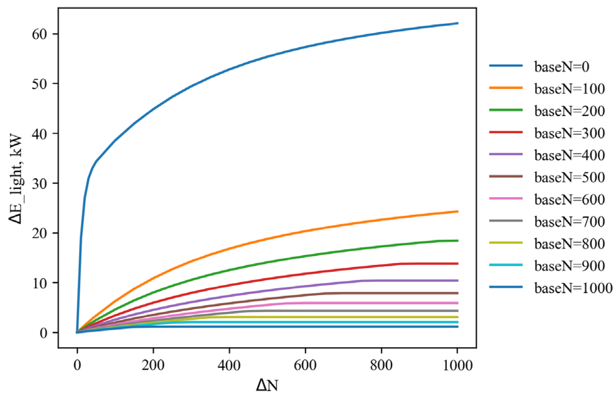
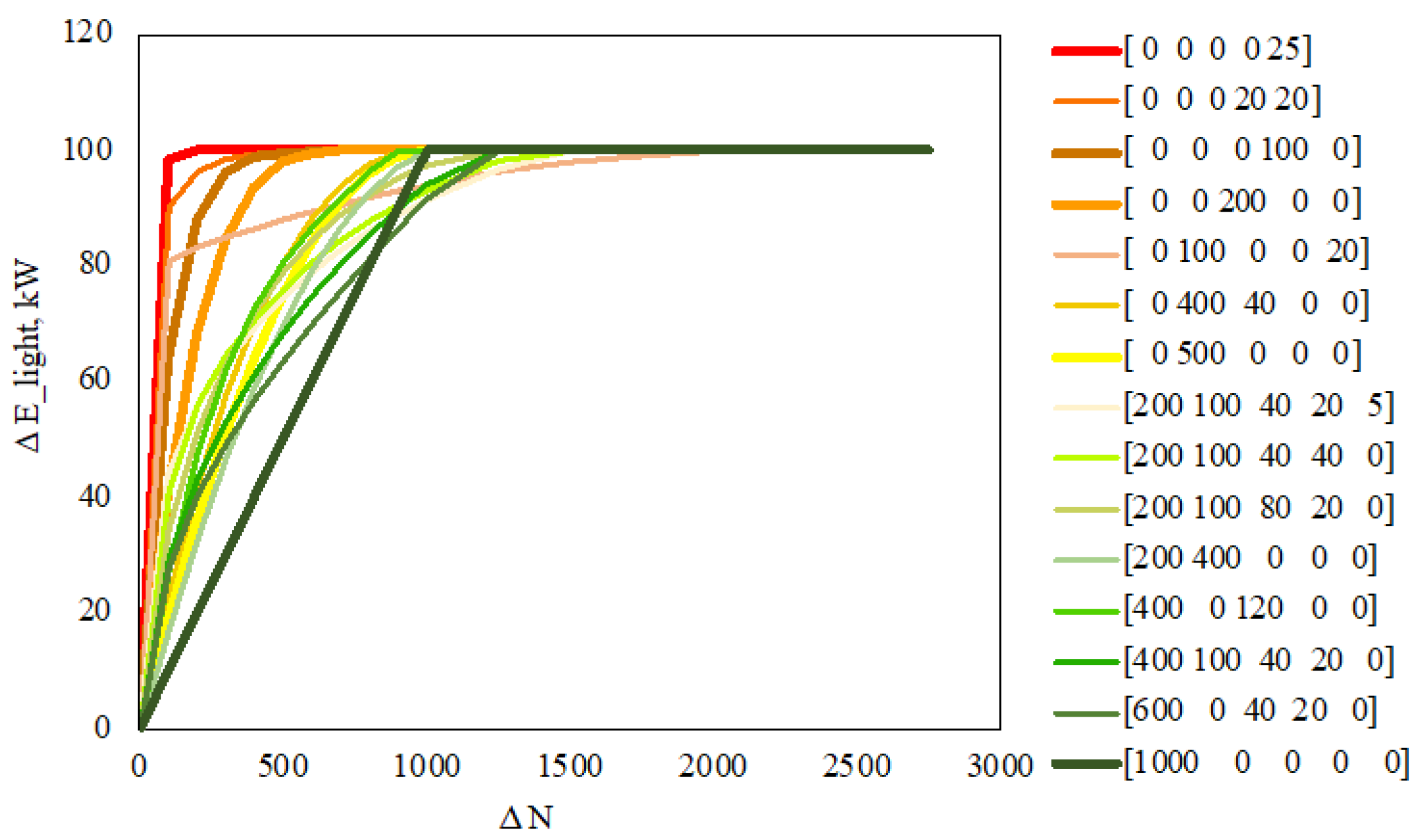
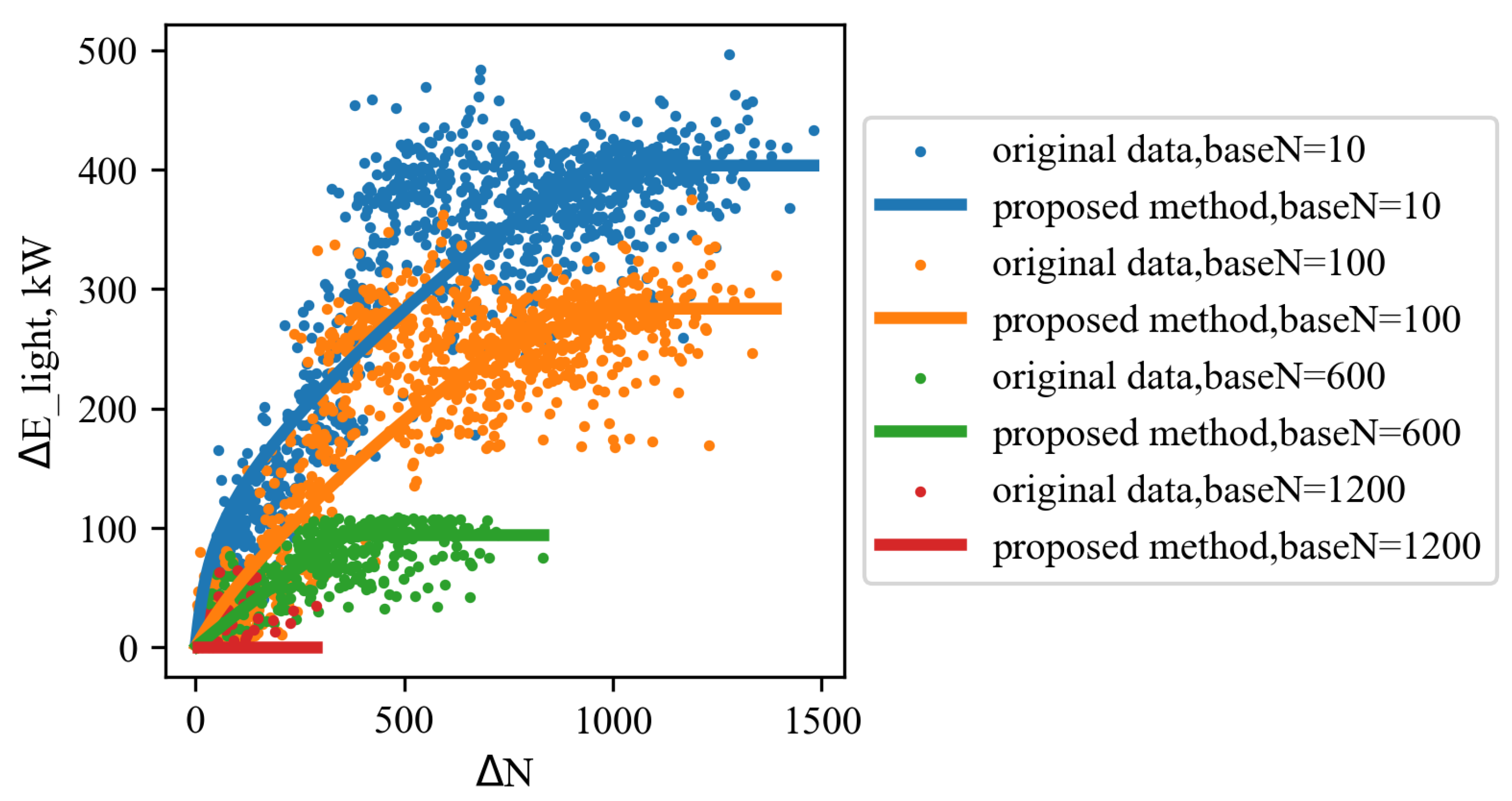
3.1.1. Lighting Energy Consumption

Figure 7 shows how lighting energy consumption change with occupancy at different existing occupancy levels. It can be seen that the more existing occupants in the building, the smaller the change in lighting energy consumption with occupancy. When baseN is 0, ∆E_light increases fast with ∆N at first and then slows down. When baseN is 500 (accounting for 43% of totalN), the maximum ∆E_light caused by occupancy is 7.85 kW (only accounting for 12.4% of total lighting energy consumption).

To simulate the influence of occupancy on the lighting energy consumption with different building layouts, it is assumed that building area, ρ_equip, totalN and baseN are the same for different layouts. Scenarios are considered in which the building contains single rooms, 2-person rooms, 6-person rooms, 10-person rooms and 40-person rooms (roomN = 1, 2, 6, 10 and 40) with different combinations of the number of each type of room (n1, n2, n5, n10 and n40). The results are shown in Figure 8.

For a building with only single rooms, represented by the curve of [1000, 0, 0, 0, 0], ∆E_light increases linearly with ∆N and then stabilizes when all the rooms are occupied. For a building with a large amount of open working space, represented by the curve of [0, 0, 0, 0, 25], ∆E_light approaches the upper limit rapidly and stays steady as the occupancy increases. If there are more private rooms, such as single rooms and two-person rooms, in the building, ∆E_light increases smoothly with ∆N.

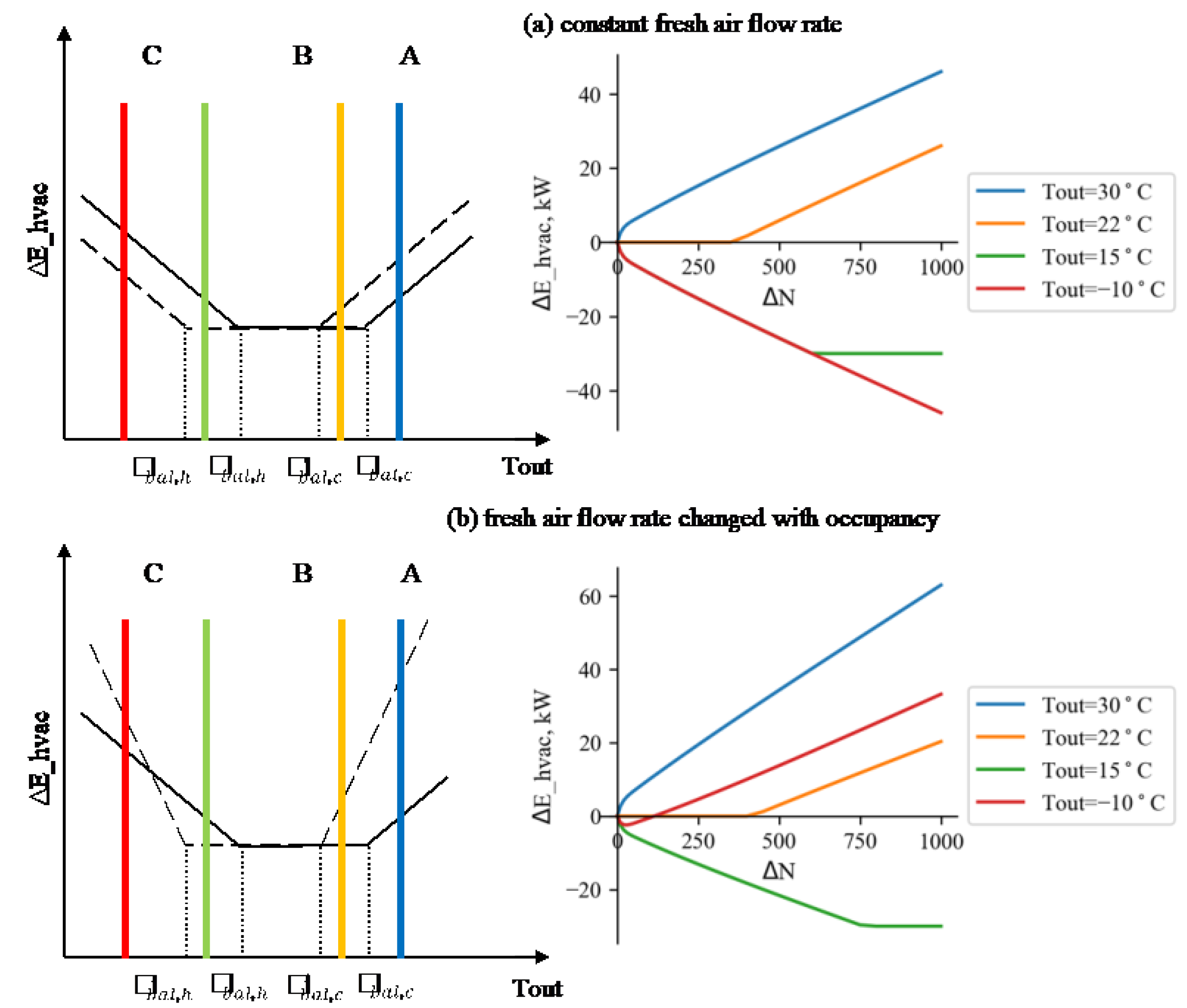
3.1.2. HVAC Energy Consumption

Figure 9 shows the influence of occupancy on ∆E_hvac at different T_out with different fresh air control strategies: (a) constant fresh air volume and (b) fresh air volume changed with occupancy. It is assumed that the existing occupancy is 0. Sections A, B and C in Figure 7 represent the situations in cooling, transition and heating conditions, respectively.

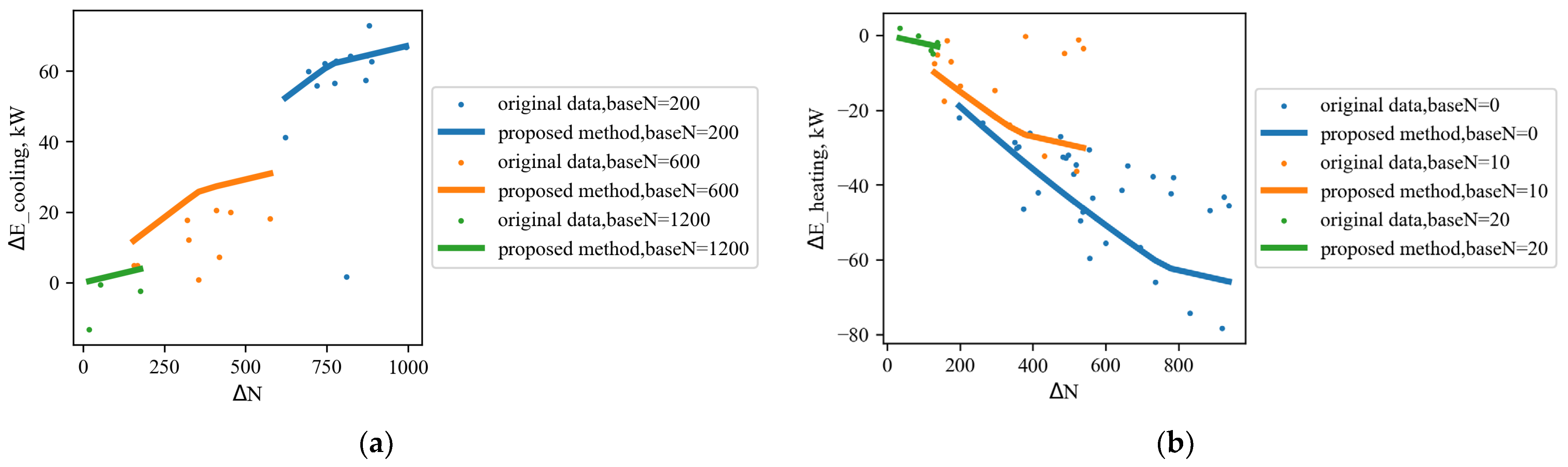
• When the building is in the cooling condition (T_out > T_bal,c), ∆E_hvac increases with ∆N, as shown by the blue line corresponding to T_out = 30 °C. In scenario (a), K_tot does not change with occupancy, so values of ∆E_hvac at different T_out are the same as long as T_out > T_bal,c. In scenario (b), K_tot would change with occupancy and ∆E_hvac would increase with T_out.
• When the building is in the transition condition (T_bal,h < T_out < T_bal,c), ∆E_hvac remains unchanged until T_out > ${\mathrm{T}}_{\mathrm{b}\mathrm{a}\mathrm{l},\mathrm{c}}^{\prime }$. Then, it increases as the occupancy increases, because extra internal load needs to be eliminated, as shown in the orange line corresponding to T_out = 22 °C.
• When the building is in the heating condition (T_out < T_bal,h), the results in scenario (a) and (b) are different. In scenario (a), ∆E_hvac decreases with increasing occupancy, then remains stable. This is because the increase in the internal load offsets a part of the heating load. However, in scenario (b), increasing occupancy would bring in both internal cooling load and fresh air heating load. When T_out is close to T_bal,h, the extra internal cooling load is larger than the fresh air heating load. ∆E_hvac decreases with increasing occupancy and then remains stable, as shown by the green line with T_out = 15 °C. When T_out is much lower than T_bal,h, ∆E_hvac increases with occupancy rapidly after a small and short decline, as shown by the red line with T_out = −10 °C. A small and short decline happens when the ∆E_light is large, which contributes to a lot of internal cooling load. As occupancy increases, the extra fresh air heating load would exceed the internal cooling load.

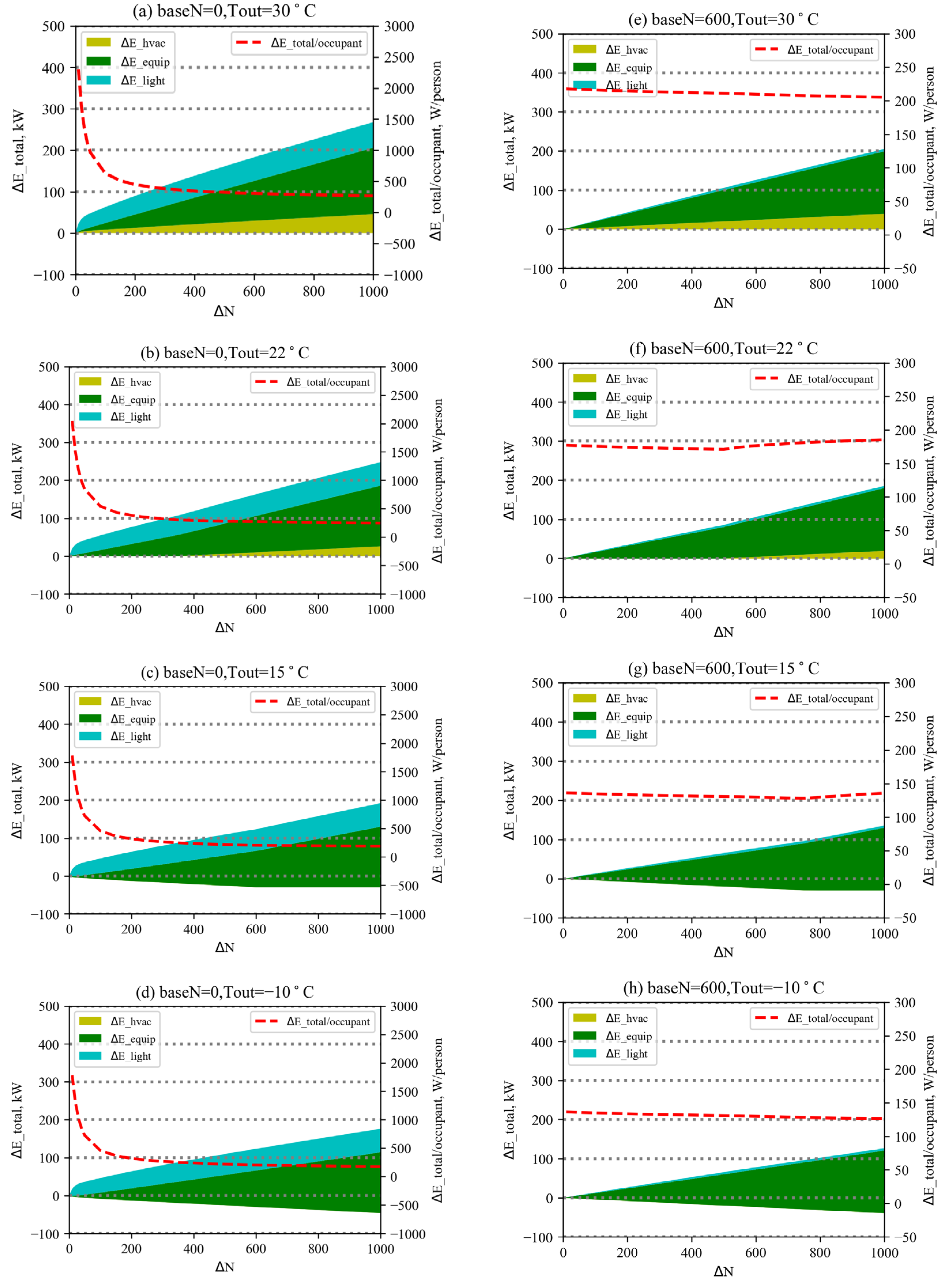
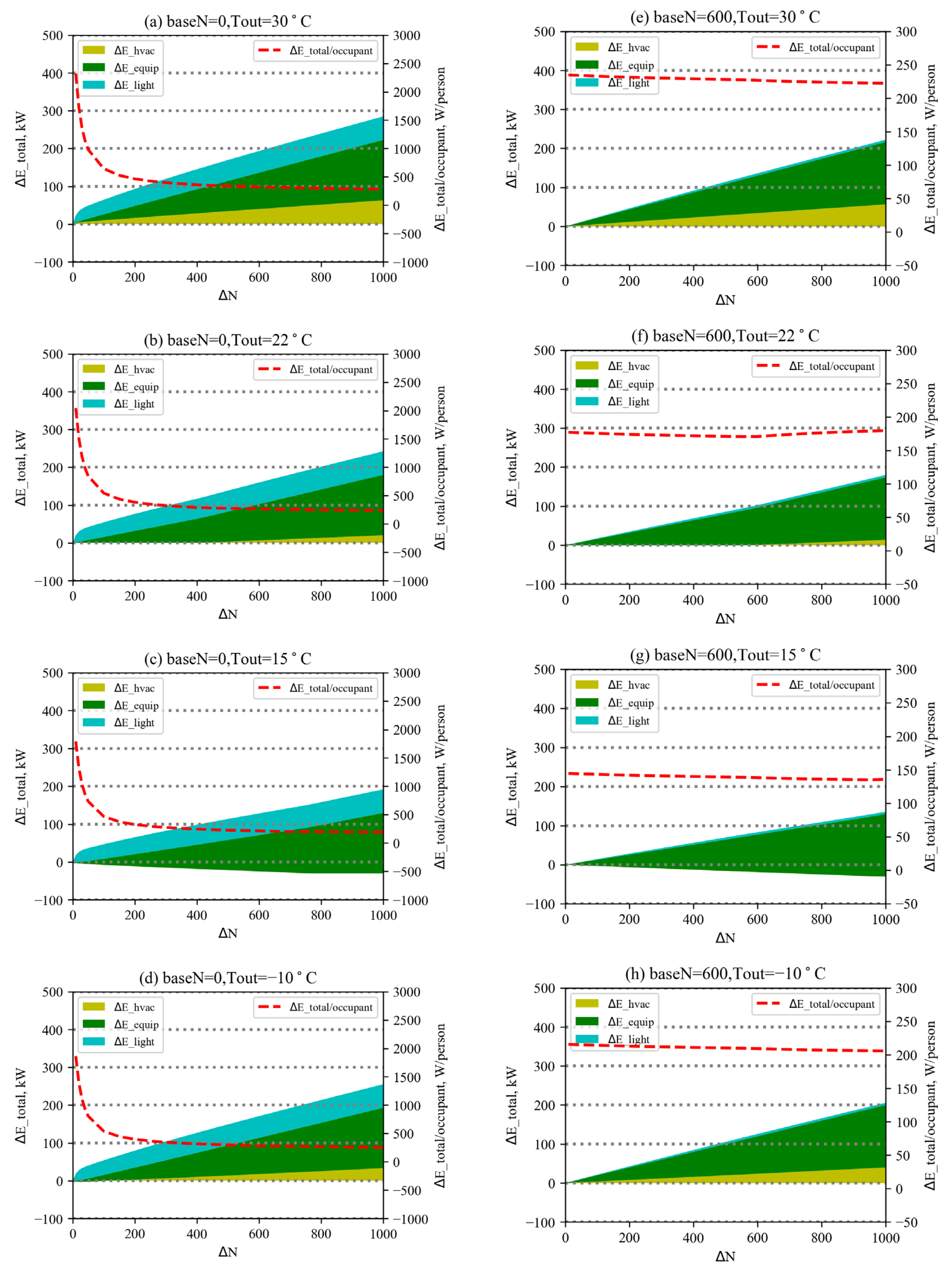
3.1.3. The Total Energy Consumption

Figure 10 and Figure 11 show the influence of occupancy on the change in total energy consumption with the constant fresh air volume control strategy and the variable fresh air volume control strategy, respectively. The results with different baseN (0 and 600) and T_out (30 °C, 22 °C, 15 °C and −10 °C) are calculated in each scenario. The left y-axis of the figures shows the change in total energy consumption, and the right y-axis shows the change in total energy consumption per person, which corresponds to the red dashed line in the figures.

When baseN is 0, the change in the lighting energy consumption is dominant. ∆E_total/occupant drops rapidly when ∆N is small and then and declines steadily to less than 500 W/person. When baseN is 600, accounting for more than half of the total number of 1160 occupants, the occupancy’s influence on ∆E_light is limited, and ∆E_total/occupant changes slightly with ∆N. ∆E_total/occupant is also related to T_out. In the constant fresh air volume scenario, ∆E_total/occupant in cooling condition > ∆E_total/occupant in transition condition > ∆E_total/occupant in heating condition.

When the fresh air volume is controlled with occupancy, ∆E_total/occupant in transition condition is smaller than that in cooling and heating conditions, which is different from the constant fresh air volume scenario. This is because in heating conditions, the fresh air heating load brought by new occupants would exceed the internal cooling load, which causes more heating energy consumption. So the ∆E_total/occupant in heating condition is larger than that in transition condition.

It is worth noting that the ∆E_total/occupant changes little with ∆N when existing occupancy exceeds half of total occupancy in the building. For most commercial buildings using the constant fresh air volume control strategy, ∆E_total/occupant would not change with T_out as long as the HVAC condition does not change. Thus, it is feasible to used two constant influence intensities to calculate occupancy impact on building energy consumption in cooling and heating conditions separately. In the transition condition, ∆E_total/occupant changes with T_out, and it causes a large calculation error when using the constant influence intensity method. For buildings using the variable fresh air volume control strategy, the constant influence intensity method is not suitable because ∆E_total/occupant would change with T_out throughout the year.

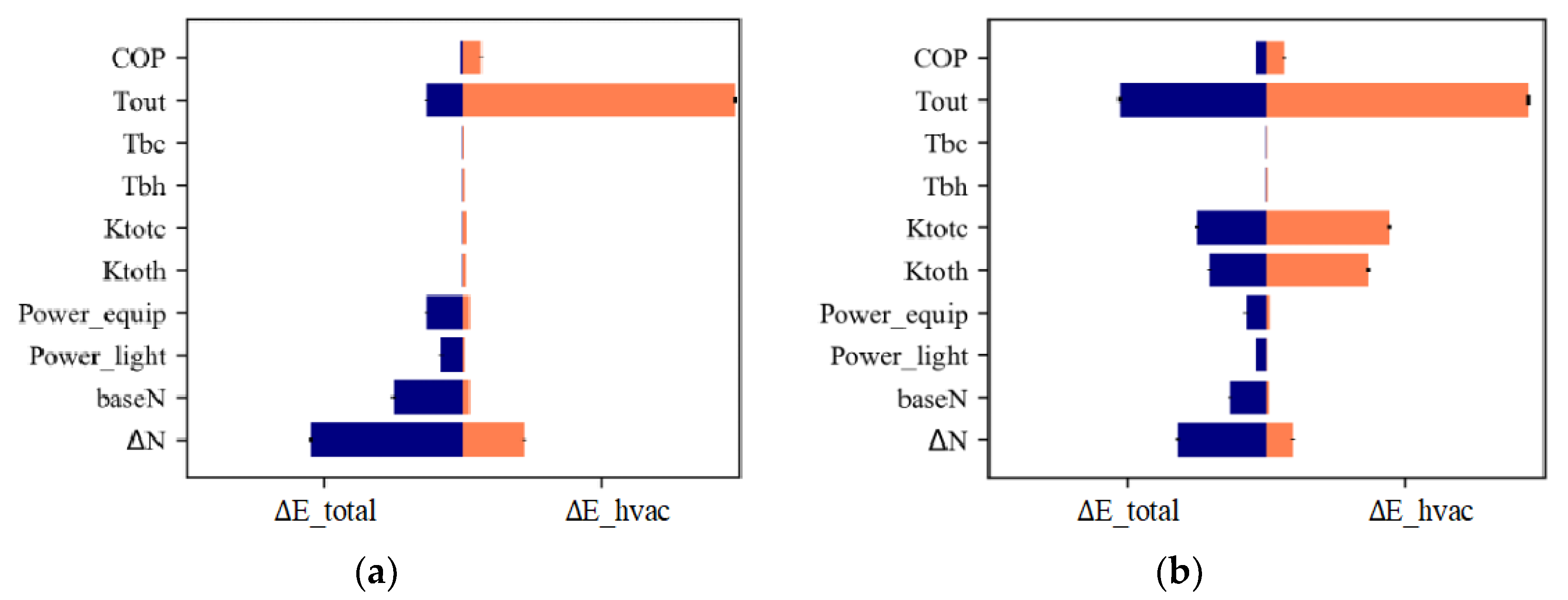
3.2. Sensitivity Analysis Results

Figure 12 shows the total effect indices for the main inputs in the proposed method on ∆E_total and ∆E_hvac in two different scenarios: (a) occupants can change K_tot and (b) occupants cannot change K_tot. The closer the bars of the histogram are to the border, the closer the index values are to 1 and thus the more important the inputs are.

In scenario (a), ∆N, baseN and T_out are the three most important factors for ∆E_total, while T_out, ∆N and COP are the most important for ∆E_hvac. T_out plays a significant role in the change in HVAC energy, but it has a lesser impact when the utilization of lighting and electric devices is taken into consideration. The baseN parameter mainly affects the lighting energy consumption, and thus it has little influence on the HVAC energy. The balance point temperature has little effect on ∆E_hvac because the balance point temperatures only have an influence when the heating or cooling conditions are changed. For example, if there is initially no need for cooling but with the increasing occupancy, T_bal,c decreases to less than T_out, then the extra cooling load should be eliminated. However, if the building is already in the cooling condition, T_bal,c would not influence ∆E_hvac. K_tot,h and K_tot,c also have little effect on ∆E_hvac because, in this scenario, ∆E_hvac is only related to ΔQ_{inter,sensible} when the heating or cooling conditions are not changed. If the heating or cooling conditions are changed, particularly in the transition season, K_tot influences T_bal and further influences ∆E_hvac.

However, in scenario (b), the facility manager could change the ventilation according to the change of the number of people, and the occupants could also change K_tot by opening windows, opening shading devices and other actions. T_out, K_tot and ∆N are the main factors affecting ∆E_hvac and ∆E_total.

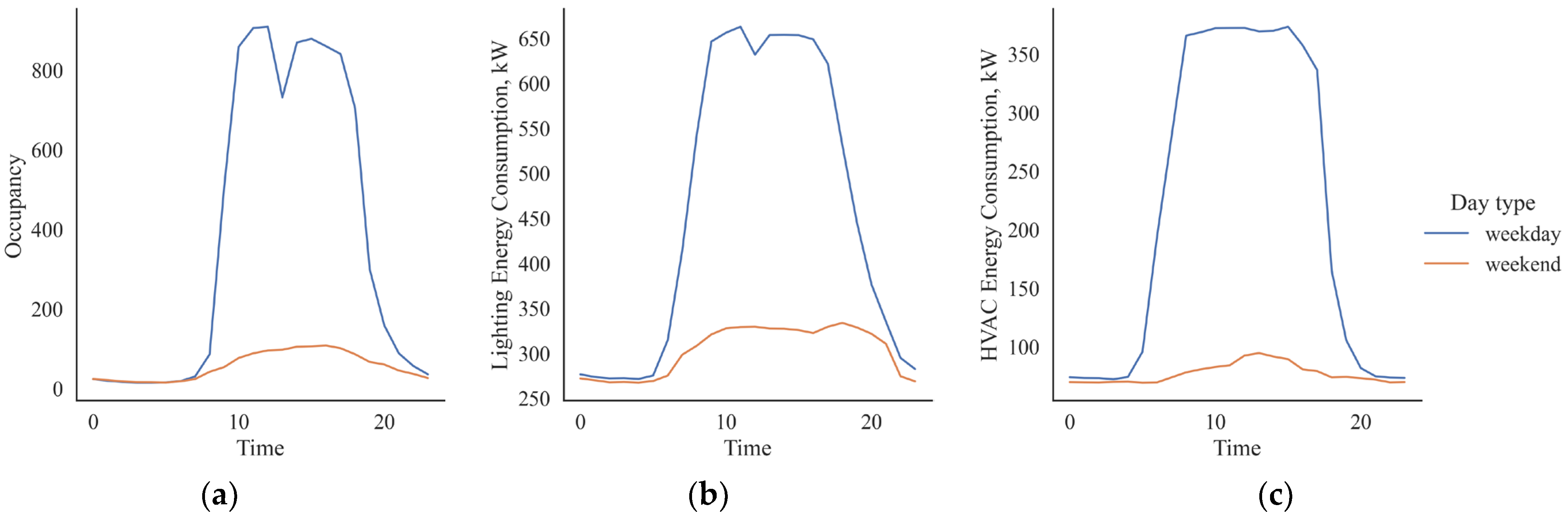
3.3. Case Study Results

Figure 13 shows the comparison of ∆E_light calculated by the proposed method with actual data based on different baseN. The coefficient of determination R² between the calculated results and the actual data is 0.86.

Figure 14 shows the comparison of ∆E_hvac in cooling and heating conditions calculated by proposed method using actual data based on different values of baseN. In the cooling condition, T_out is set as 32 °C because the actual data at 32 °C are more than those at other T_out and can thus be used to validate the proposed method. The R² between the calculated results and the actual data is 0.8. In the heating condition, T_out is set as 11 °C and the R² is 0.71.

The total calculation time of the proposed method in this study is only 7.4 s. It is therefore very fast and convenient to calculate the change in building energy consumption with occupancy. Although this method cannot reflect the stochastic variation caused by occupants, it is very useful in commercial building energy control and assessments.

4. Discussion

Building layout and existing occupancy level are two main factors affecting occupancy’s influence on building energy consumption. However, these two factors have usually been ignored in previous research. The reason is that most researches used BPS tools to simulate the impact of occupancy, so it is rather labor-intensive to generate numerous BPS models with different layouts. In our proposed method, these two factors were used to calculate the probability that new occupants enter certain rooms in a building. It is very convenient for calculating occupancy’s influence in different layouts under existing occupancy levels. And it is very useful in energy comparison between different buildings.

In our proposed method, the influence of occupancy and other occupant behaviors on HVAC energy consumption are simplified into the balance temperature and the total heat transmission coefficient of the building. So, it can be used to calculate occupancy’ influence with different occupant-related control strategies, such as fresh air control, thermostat control shading control and so on. However, in this paper, we only compare the occupancy’ influence in different fresh air control strategies. The calculation results in Section 3.1.3 further prove that a constant influence intensity cannot reflect occupancy influence’ on building energy consumption exactly because occupancy influence intensity is also related to outdoor air temperature. However, for commercial buildings with constant fresh air control, it is feasible to use two constant influence intensities to calculate occupancy impact on building energy consumption in cooling and heating conditions separately.

The case study results show that the proposed method performs well in calculating ∆E_light caused by changing occupancy for different existing occupancies. The errors might come from three problems: (1) the proposed method calculated the expected value of ∆E_light, which does not reflect stochastic situations; (2) the proposed method only considers the change in occupancy at the whole building level and cannot be used to calculate energy change caused by occupant movement in the building; and (3) in the actual situation, some occupants might leave without turning off the light or turn on the light according to the illumination level. However, in this case study, the light control strategy is assumed as turning the light on when an occupant arrives and turning it off when they leave.

The calculation results in heating and cooling energy consumption are worse than lighting. The errors might come from four issues: (1) the error propagated from the lighting sector; (2) the solar heat gain is assumed to be unchanged with occupancy in the proposed method; (3) K_tot is assumed as a constant value in this case study when, in the actual situation, occupants might open windows or adjust shading devices; (4) and the HVAC system’s energy consumption is also related to the control strategy of HVAC equipment. In an ideal case, the HVAC equipment control strategy, such as the number of chillers in operation, should change with the cooling and heating load. However, the HVAC equipment controls in practice are usually rough. The proposed method only considers the ideal control case, while the practical control strategy is ignored.

5. Conclusions

Occupancy is one of the most important factors for commercial building energy consumption. It is important for both building managers and energy simulation engineers to know how the entire building’s energy consumption varies with occupancy in BA system control, different building performance comparison and building energy efficiency assessment. This study proposes a fast method for calculating occupancy impact on commercial building energy consumption at the whole building level. The case study results show that the proposed method performs well in practice.

The main advantages of the proposed method include:

• The building layout and existing occupancy are taken into consideration, which have generally been ignored in previous studies;
• A physical building energy model is not needed for the proposed method. Thus, it is very fast and convenient to calculate the occupancy’s influence on the energy consumption of different commercial buildings in different scenarios;
• There are not too many input parameters, and they are easy to obtain from building CAD drawings and existing building energy management systems.

The limitations of the proposed method are:

• It is not a stochastic method, and the occupant diversity is not considered. The expected value of building energy change is calculated, which does not reflect stochastic situations. Thus, this method is only suitable for commercial buildings, not for residential buildings;
• The proposed method only considers the change in occupancy at the whole building level. It cannot be used to calculate energy changes caused by occupant movement in the building;
• Because this study focuses on the energy consumption at the whole building level, a simplified method is used for the calculation of heating and cooling loads. Therefore, the proposed method is not suitable for cases with short time intervals or small spatial scales.

In this study, the HVAC equipment is assumed to operate with an ideal control strategy. How to apply the proposed method with different HVAC control strategies should be further researched. Moreover, the influence of occupant behaviors on building energy consumption is comprehensively reflected in the T_bal and K_tot parameters. The relationship between these two parameters and occupant behaviors, such as window/shading control, should be further investigated to supplement the proposed method.

References

1. EIA. International Energy Outlook 2021; EIA: Washington, DC, USA, 2021.
2. THUBERC. Annual Report on China Building Energy Efficiency; Energy Foundation: Beijing, China, 2022; ISBN 978-7-112-27194-8. [Google Scholar]
3. Hong, T.; Taylor-Lange, S.C.; D’Oca, S.; Yan, D.; Corgnati, S.P. Advances in Research and Applications of Energy-Related Occupant Behavior in Buildings. Energy Build. 2016, 116, 694–702. [Google Scholar] [CrossRef] [Green Version]
4. Da, Y.; Tianzhen, H. Annex 66 Final Report: Definition and Simulation of Occupant Behavior in Buildings; International Energy Agency: Paris, France, 2018. [Google Scholar]
5. O’Brien, W.; Wagner, A.; Schweiker, M.; Mahdavi, A.; Day, J.; Kjærgaard, M.B.; Carlucci, S.; Dong, B.; Tahmasebi, F.; Yan, D.; et al. Introducing IEA EBC Annex 79: Key Challenges and Opportunities in the Field of Occupant-Centric Building Design and Operation. Build. Environ. 2020, 178, 106738. [Google Scholar] [CrossRef]
6. Page, J.; Robinson, D.; Morel, N.; Scartezzini, J.L. A Generalised Stochastic Model for the Simulation of Occupant Presence. Energy Build. 2008, 40, 83–98. [Google Scholar] [CrossRef]
7. Wang, C.; Yan, D.; Jiang, Y. A Novel Approach for Building Occupancy Simulation. Build. Simul. 2011, 4, 149–167. [Google Scholar] [CrossRef]
8. D’Oca, S.; Hong, T. Occupancy Schedules Learning Process through a Data Mining Framework. Energy Build. 2015, 88, 395–408. [Google Scholar] [CrossRef] [Green Version]
9. Jiefan, G.; Peng, X.; Zhihong, P.; Yongbao, C.; Ying, J.; Zhe, C. Extracting Typical Occupancy Data of Different Buildings from Mobile Positioning Data. Energy Build. 2018, 180, 135–145. [Google Scholar] [CrossRef]
10. Hunt, D.R.G. Predicting Artificial Lighting Use—A Method Based upon Observed Patterns of Behaviour. Light. Res. Technol. 1980, 12, 7–14. [Google Scholar] [CrossRef]
11. Reinhart, C.F. Lightswitch-2002: A Model for Manual and Automated Control of Electric Lighting and Blinds. Sol. Energy 2004, 77, 15–28. [Google Scholar] [CrossRef] [Green Version]
12. Wang, C.; Yan, D.; Sun, H.; Jiang, Y. A Generalized Probabilistic Formula Relating Occupant Behavior to Environmental Conditions. Build. Environ. 2016, 95, 53–62. [Google Scholar] [CrossRef]
13. Zhou, X.; Yan, D.; Hong, T.; Ren, X. Data Analysis and Stochastic Modeling of Lighting Energy Use in Large Office Buildings in China. Energy Build. 2015, 86, 275–287. [Google Scholar] [CrossRef] [Green Version]
14. Richardson, I.; Thomson, M.; Infield, D.; Clifford, C. Domestic Electricity Use: A High-Resolution Energy Demand Model. Energy Build. 2010, 42, 1878–1887. [Google Scholar] [CrossRef] [Green Version]
15. Haldi, F.; Robinson, D. On the Behaviour and Adaptation of Office Occupants. Build. Environ. 2008, 43, 2163–2177. [Google Scholar] [CrossRef]
16. Gunay, H.B.; O’Brien, W.; Beausoleil-Morrison, I.; Bursill, J. Development and Implementation of a Thermostat Learning Algorithm. Sci. Technol. Built Environ. 2018, 24, 43–56. [Google Scholar] [CrossRef]
17. Haldi, F.; Robinson, D. Interactions with Window Openings by Office Occupants. Build. Environ. 2009, 44, 2378–2395. [Google Scholar] [CrossRef]
18. Langevin, J.; Wen, J.; Gurian, P.L. Simulating the Human-Building Interaction: Development and Validation of an Agent-Based Model of Office Occupant Behaviors. Build. Environ. 2015, 88, 27–45. [Google Scholar] [CrossRef]
19. Inkarojrit, V. Monitoring and Modelling of Manually-Controlled Venetian Blinds in Private Offices: A Pilot Study. J. Build. Perform. Simul. 2008, 1, 75–89. [Google Scholar] [CrossRef]
20. Jin, Y.; Yan, D.; Chong, A.; Dong, B.; An, J. Building Occupancy Forecasting: A Systematical and Critical Review. Energy Build. 2021, 251, 111345. [Google Scholar] [CrossRef]
21. Zou, H.; Zhou, Y.; Jiang, H.; Chien, S.-C.; Xie, L.; Spanos, C.J. WinLight: A WiFi-Based Occupancy-Driven Lighting Control System for Smart Building. Energy Build. 2018, 158, 924–938. [Google Scholar] [CrossRef]
22. Tekler, Z.D.; Low, R.; Yuen, C.; Blessing, L. Plug-Mate: An IoT-Based Occupancy-Driven Plug Load Management System in Smart Buildings. Build. Environ. 2022, 223, 109472. [Google Scholar] [CrossRef]
23. Balaji, B.; Xu, J.; Nwokafor, A.; Gupta, R.; Agarwal, Y. Sentinel. In Proceedings of the 11th ACM Conference on Embedded Networked Sensor Systems, Rome, Italy, 11–15 November 2013; ACM: New York, NY, USA, 2013; pp. 1–14. [Google Scholar]
24. Beltran, A.; Cerpa, A.E. Optimal HVAC Building Control with Occupancy Prediction. In Proceedings of the 1st ACM Conference on Embedded Systems for Energy-Efficient Buildings, Memphis, TN, USA, 3–6 November 2014; ACM: New York, NY, USA, 2014; pp. 168–171. [Google Scholar]
25. Agarwal, Y.; Balaji, B.; Dutta, S.; Gupta, R.K.; Weng, T. Duty-Cycling Buildings Aggressively: The next Frontier in HVAC Control. In Proceedings of the 10th ACM/IEEE International Conference on Information Processing in Sensor Networks, Chicago, IL, USA, 12–14 April 2011; pp. 246–257. [Google Scholar]
26. Kong, M.; Dong, B.; Zhang, R.; O’Neill, Z. HVAC Energy Savings, Thermal Comfort and Air Quality for Occupant-Centric Control through a Side-by-Side Experimental Study. Appl. Energy 2022, 306, 117987. [Google Scholar] [CrossRef]
27. Erickson, V.L.; Carreira-Perpiñán, M.Á.; Cerpa, A.E. OBSERVE: Occupancy-Based System for Efficient Reduction of HVAC Energy. In Proceedings of the 10th ACM/IEEE International Conference on Information Processing in Sensor Networks, Chicago, IL, USA, 12–14 April 2011; pp. 258–269. [Google Scholar]
28. Ding, Y.; Han, S.; Tian, Z.; Yao, J.; Chen, W.; Zhang, Q. Review on Occupancy Detection and Prediction in Building Simulation. Build. Simul. 2022, 15, 333–356. [Google Scholar] [CrossRef]
29. Floyd, D.B.; Parker, D.S.; Sherwin, J.R. Measured Field Performance and Energy Savings of Occupancy Sensors: Three Case Studies. Florida Sol. Energy Cent. 2002, 97–105. [Google Scholar]
30. Benezeth, Y.; Laurent, H.; Emile, B.; Rosenberger, C. Towards a Sensor for Detecting Human Presence and Characterizing Activity. Energy Build. 2011, 43, 305–314. [Google Scholar] [CrossRef]
31. Wang, S.; Burnett, J.; Chong, H. Experimental Validation of CO2-Based Occupancy Detection for Demand-Controlled Ventilation. Indoor Built Environ. 1999, 8, 377–391. [Google Scholar] [CrossRef]
32. Vafeiadis, T.; Zikos, S.; Stauropoulos, G.; Ioannidis, D.; Moustakas, K. Machine Learning Based Occupancy Detection Via the Use of Smart Meters. In Proceedings of the International Conference on Energy Science and Electrical Engineering (ICESEE), Budapest, Hungary, 20–22 October 2016. [Google Scholar]
33. Tekler, Z.D.; Chong, A. Occupancy Prediction Using Deep Learning Approaches across Multiple Space Types: A Minimum Sensing Strategy. Build. Environ. 2022, 226, 109689. [Google Scholar] [CrossRef]
34. Depatla, S.; Muralidharan, A.; Mostofi, Y. Occupancy Estimation Using Only WiFi Power Measurements. IEEE J. Sel. Areas Commun. 2015, 33, 1381–1393. [Google Scholar] [CrossRef]
35. Tekler, Z.D.; Low, R.; Gunay, B.; Andersen, R.K.; Blessing, L. A Scalable Bluetooth Low Energy Approach to Identify Occupancy Patterns and Profiles in Office Spaces. Build. Environ. 2020, 171, 106681. [Google Scholar] [CrossRef]
36. Lu, X.; Feng, F.; Pang, Z.; Yang, T.; O’Neill, Z. Extracting Typical Occupancy Schedules from Social Media (TOSSM) and Its Integration with Building Energy Modeling. Build. Simul. 2021, 14, 25–41. [Google Scholar] [CrossRef]
37. Hong, T.; Sun, H.; Chen, Y.; Taylor-Lange, S.C.; Yan, D. An Occupant Behavior Modeling Tool for Co-Simulation. Energy Build. 2016, 117, 272–281. [Google Scholar] [CrossRef] [Green Version]
38. Jia, M.; Srinivasan, R.; Ries, R.; Bharathy, G.; Weyer, N. Investigating the Impact of Actual and Modeled Occupant Behavior Information Input to Building Performance Simulation. Buildings 2021, 11, 32. [Google Scholar] [CrossRef]
39. Sha, H.; Xu, P.; Yan, C.; Ji, Y.; Zhou, K.; Chen, F. Development of a Key-Variable-Based Parallel HVAC Energy Predictive Model. Build. Simul. 2022, 15, 1193–1208. [Google Scholar] [CrossRef]
40. Amasyali, K.; El-Gohary, N. Machine Learning for Occupant-Behavior-Sensitive Cooling Energy Consumption Prediction in Office Buildings. Renew. Sustain. Energy Rev. 2021, 142, 110714. [Google Scholar] [CrossRef]
41. Amasyali, K.; El-Gohary, N.M. Real Data-Driven Occupant-Behavior Optimization for Reduced Energy Consumption and Improved Comfort. Appl. Energy 2021, 302, 117276. [Google Scholar] [CrossRef]
42. Selvacanabady, A.; Judd, K. The Influence of Occupancy on Building Energy Use Intensity and the Utility of an Occupancy-Adjusted Performance Metric (PNNL-26019); US Department of Energy: Washington, DC, USA, 2017.
43. Kim, Y.S.; Srebric, J. Impact of Occupancy Rates on the Building Electricity Consumption in Commercial Buildings. Energy Build. 2017, 138, 591–600. [Google Scholar] [CrossRef]
44. Raghavendra Rao, A.; Mahesh, M. Analysis of the Energy and Safety Critical Traction Parameters for Elevators. EPE J. 2018, 28, 169–181. [Google Scholar] [CrossRef]
45. Kim, Y.S.; Srebric, J. Improvement of Building Energy Simulation Accuracy with Occupancy Schedules Derived from Hourly Building Electricity Consumption. ASHRAE Conf. 2015, 121, 353–360. [Google Scholar]
46. Strand, R.K. ASHREA Handbook. Fundamentals; ASHRAE: Peachtree Corners, GA, USA, 2009; ISBN 978-1-936504-45-9. [Google Scholar]
47. Karlsson, J.; Roos, A.; Karlsson, B. Building and Climate Influence on the Balance Temperature of Buildings. Build. Environ. 2003, 38, 75–81. [Google Scholar] [CrossRef]
48. Zhao, R.; Fan, C.; Xue, D.; Qian, Y. Air Conditioning; Architecture and Building Press: Beijing, China, 2008. [Google Scholar]
49. Saltelli, A.; Annoni, P.; Azzini, I.; Campolongo, F.; Ratto, M.; Tarantola, S. Variance Based Sensitivity Analysis of Model Output. Design and Estimator for the Total Sensitivity Index. Comput. Phys. Commun. 2010, 181, 259–270. [Google Scholar] [CrossRef]
50. Herman, J.; Usher, W. SALib: An Open-Source Python Library for Sensitivity Analysis. J. Open Source Softw. 2017, 2, 97. [Google Scholar] [CrossRef]
51. ASHRAE. 90.1-2013 User’s Manual: ANSI/ASHRAE/IES Standard 90.1, Energy Standard for Buildings Except Low-Rise Residential Buildings; ASHRAE: Peachtree Corners, GA, USA, 2013. [Google Scholar]
52. Tekler, Z.D.; Ono, E.; Peng, Y.; Zhan, S.; Lasternas, B.; Chong, A. ROBOD, Room-Level Occupancy and Building Operation Dataset. Build. Simul. 2022, 15, 2127–2137. [Google Scholar] [CrossRef]
Figure 1. Influences of occupant behaviors on building energy consumption.
Buildings 13 00567 g001
Figure 2. Influences of occupant behavior on building energy per occupant with occupancy under different building automation levels [4].
Buildings 13 00567 g002
Figure 3. Basic structure of the proposed method.
Buildings 13 00567 g003
Figure 4. Illustration of two different building layouts: (a) 10 single-person rooms; (b) 2 five-person rooms.
Buildings 13 00567 g004
Figure 5. (a) Study building and (b) building layout of one floor.
Buildings 13 00567 g005
Figure 6. (a) Average daily occupancy, (b) average daily lighting energy consumption and (c) average daily HVAC energy consumption.
Buildings 13 00567 g006
Figure 7. Influence of ∆N on ∆Elight at different existing occupancy levels.
Buildings 13 00567 g007
Figure 8. Influence of ∆N on ∆Elight at different building layouts (baseN = 0).
Buildings 13 00567 g008
Figure 9. Influence of ∆N on ∆Ehvac at different Tout with different fresh air control strategies: (a) constant fresh air volume and (b) fresh air volume changed with occupancy.
Buildings 13 00567 g009
Figure 10. The influence of occupancy on the change in total energy consumption with different baseN and Tout (constant fresh air volume).
Buildings 13 00567 g010
Figure 11. The influence of occupancy on the change in total energy consumption with different baseN and Tout (variable fresh air volume).
Buildings 13 00567 g011
Figure 12. Total effect indices for the main inputs on ∆Etotal and ∆Ehvac in two different scenarios: (a) occupants can change Ktot and (b) occupants cannot change Ktot.
Buildings 13 00567 g012
Figure 13. Comparison of ∆Elight calculated by the proposed method and actual data.
Buildings 13 00567 g013
Figure 14. Comparison of ∆Ehvac calculated by the proposed method and actual data in (a) cooling, condition (Tout = 32 °C) and (b) heating condition (Tout = 11 °C).
Buildings 13 00567 g014