Bayesian Optimization Framework for HVAC System Control

Abstract

The use of machine-learning algorithms in optimizing the energy efficiency of HVAC systems has been widely studied in recent years. Previous research has focused mainly on data-driven model predictive controls and reinforcement learning. Both approaches require a large amount of online interactive data; therefore, they are not efficient and stable enough for large-scale practical applications. In this paper, a Bayesian optimization framework for HVAC control has been proposed to achieve near-optimal control performance while also maintaining high efficiency and stability, which would allow it to be implemented in a large number of projects to obtain large-scale benefits. The proposed framework includes the following: (1) a method for modeling HVAC control problems as contexture Bayesian optimization problems and a technology for automatically constructing Bayesian optimization samples, which are based on time series raw trending data; (2) a Gaussian process regression surrogate model for the objective function of optimization; (3) a Bayesian optimization control loop, optimized for the characteristics of HVAC system controls, including an additional exploration trick based on noise estimation and a mechanism to ensure constraint satisfaction. The performance of the proposed framework was evaluated by using a simulation system, which was calibrated by using trending data from a real data center. The results of our study showed that the proposed approach achieved more than a 10% increase in energy-efficiency savings within a few weeks of optimization time compared with the original building automation control.

1. Introduction

The substantial energy consumption of heating, ventilation and air-conditioning (HVAC) systems means that it is important to optimize their energy efficiency. Optimal control methods for HVAC systems that are driven by machine learning have been widely studied recently, particularly data-driven model predictive control (MPC) and reinforcement learning (RL). Maddalena et al. [1] and Zhang et al. [2] conducted thorough reviews in these fields. It has been found that owing to their high model complexity and low data efficiency, it is still difficult to deploy them in a wide range of practical HVAC systems at a low cost. There have also been studies on the Bayesian optimization of HVAC controls, as it is an efficient black-box optimization method. The main objective of this paper is to introduce the work related to the Bayesian optimization of HVAC controls and to propose an efficient framework.

Most previous studies on the use of Bayesian optimization for HVAC controls have focused on the use of Bayesian optimization to assist the hyperparameter optimization of other underlying control algorithms, such as traditional proportional integral derivation (PID) control and MPC. Fiducioso et al. [3] used a Bayesian optimization approach to optimize the proportional and integral gains of a proportional integral (PI) controller in a ubiquitous room temperature control loop. In their study, the performance of the algorithm was evaluated by simulation. Lu et al. [4] used Bayesian optimization to optimize the MPC controller parameters to minimize the year-long closed-loop costs. Their simulation results showed that Bayesian optimization can find the optimal backoff terms by conducting 13-year-long simulations, which could significantly reduce the computational burden of a naive grid search. Lu [5] extended their work by introducing a reference model, which gathered the closed-loop performance of a low-complexity MPC controller through evaluation. This changed the goal of Bayesian optimization from learning the objective function to learning the residual function (the error between the reference and the objective function), which is a much easier task. The simulation results showed that the use of a reference model can assist Bayesian optimization to more judiciously sample the parameter estimate and to more quickly discover the regions in which the solution exists. Chakrabarty et al. [6] used Bayesian optimization to warm start the extremum-seeking control algorithm. The warm start increased the likelihood of attaining a global optimum for locally convex, rather than globally nonconvex, objective functions by identifying regions in which the global optimum most likely resides. Bhattacharya et al. [7] used Bayesian optimization to efficiently explore the design space and to jointly optimize both the system and the control design parameters of a commercial building—a chiller plant, which included the quantity of chillers, the chillers’ capacities and the switching thresholds for turning the chillers on/off in the chiller’s sequencing control logic. Chakrabarty et al. [8] used Bayesian optimization to calibrate the dynamic models of HVAC systems. In this case, the Bayesian optimization did not directly belong to HVAC controls; however, it could still be helpful for enabling control algorithms to rely on a system dynamic model.

Unlike the aforementioned studies, Takabatake et al. [9] used Bayesian optimization as a main control algorithm to directly control the cooling water temperature and the cooling water flow rate in a one-on-one HVAC system (one cooling tower and one chiller). To ensure the thermal comfort of the rooms, the load-side setpoints, including the chilled water temperature and the chilled water flow rate, were fixed to 7 °C and 1008 L/min, respectively. The search ranges of the cooling water temperature and the cooling water flow rate were determined by the ambient wet bulb temperature and by the chiller load factor, according to an empirical formula. The interval between changing the set values was fixed to 1 h. The training results indicated that the optimal setpoint values could be automatically determined in 4 weeks if the training proceeded under the rated specification control with Bayesian optimization.

The control performance of Bayesian optimization in assisting the hyperparameter optimization of the other underlying control algorithms was limited by the performance of the underlying control algorithm itself. The performance of Bayesian optimization in Takabatake’s study [9] was limited by the fixed control intervals and by the very restricted control variables, which excluded the important load-side setpoints. In addition, the safety of the setpoint adjustment relied only on the predefined search ranges, which lacked online safety assurance. In this study, we propose a Bayesian optimization framework for HVAC controls that can enable the direct control of the full setpoints of the water system in HVAC systems, with safety assurance. The major contributions of our work are as follows:

• A method for modeling HVAC control problems as contexture Bayesian optimization problems is proposed, and an approach for automatically constructing Bayesian optimization samples from raw time series trending data is also proposed. This approach includes automatically identifying and discarding the transition process and automatically determining the data observation duration of Bayesian optimization samples.
• A mechanism is provided to ensure its operational safety by feedforwarding a combination of constraint optimization and feedback constraint correction in the Bayesian optimization control loop. Meanwhile, an additional exploration trick, which is based on noise estimation, is also proposed and studied to make the optimization more robust in terms of noise observation.

2. Background

2.1. HVAC Systems and Their Control

A typical HVAC system can be broken down into two main subsystems: a water system and an air system. The water system consists of chillers or heat pumps that produce a cold/heat source and water circulation devices (e.g., pumps) to transfer the cold/heat source. The air system includes air-handling units (AHUs), variable air volume (VAV), boxes and fan coil units (FCUs), which regulate a space’s air conditions, such as its air temperature and humidity. A heat exchange between the water system and the air system is achieved through a heat exchanger, which is in the AHU, PAU or FCU [10].

The energy efficiency of HVAC systems can be significantly affected by their control strategies. Currently, in practice, rule-based control (RBC) is widely used to determine the setpoints of HVAC systems, such as various temperature/pressure/frequency setpoints. The rules in RBC are usually static and are determined on the basis of the experiences of engineers and facility managers. Significant energy savings can potentially be achieved if optimal control strategies are used to replace traditional building automation (BA). The control systems with tradition BA usually use static rules [11].

2.2. Sequential Decision Problem

A sequential decision problem means that at a given state vector (${\mathit{s}}_t$) and at a particular time step ($\mathrm{t}$), the selected action (${\mathit{a}}_t)$ affects not only the immediate reward until the next time step (t + 1) but also the next state (${\mathit{s}}_{t+1})$. Consequently, it indirectly affects the next action (${\mathit{a}}_{t+1}$) that will be taken and the future reward, after (t + 1). To attain the goal of achieving long-term accumulated rewards in sequential decision settings, we should take into account the future state trajectory (${\mathit{s}}_{\mathrm{t}:\mathrm{t}+\mathrm{horizon}}$) when making decisions at a time step ($\mathrm{t})$.

The main approaches that are used to handle a sequential decision problem are MPC and RL. In MPC, we construct a state transfer function ${\mathit{s}}_{\mathrm{t}+1}=f\left({\mathit{s}}_{t,}{\mathit{a}}_t\right)$ and a reward function $r_t=r\left({\mathit{s}}_t,{\mathit{a}}_t\right)$, and then we solve an h-step planning problem ${\mathit{a}}_{t:t+h-1}^{*}=\underset{{\mathit{a}}_{t:t+h+1}}{\mathrm{argmax}}\sum _{i=0}^{h-1}{r}_{t+i}$ at each time step ($\mathrm{t}$); then we discard ${\mathit{a}}_{t+1:t+h-1}^{*}$ and apply only ${\mathit{a}}_{\mathrm{t}}^{*}$ to the system control [12]. In RL, there are many approaches, such as model-based and model-free approaches and off-policy and on-policy approaches. Given the complex dynamic system optimization, which focuses on sample efficiency, off-policy and model-free approaches are widely used. This approach internally uses mainly Bellman’s optimality equation, $Q^{*}\left({\mathit{s}}_t,{\mathit{a}}_t\right)=\underset{{\mathit{s}}_{t+1}~P(·|{\mathit{s}}_t,{\mathit{a}}_t)}{\mathrm{E}}\left[r\left({\mathit{s}}_t,{\mathit{a}}_t\right)+\gamma \underset{{\mathit{a}}_{t+1}}{\max }{Q}^{*}\left({\mathit{s}}_{t+1},{\mathit{a}}_{t+1}\right)\right]$ and takes action by maximizing the optimal Q function [13]. Both MPC and RL need a large number of data to learn the complex state transfer function or the self-contained optimal Q function, which makes it difficult to apply them to practical, physical systems such as HVAC systems.

2.3. Contextual Optimization Problem

In a contextual optimization problem, the reward function $\mathrm{r}\left(\mathit{s},\mathit{a}\right)$ to be optimized consists of two types of variables: state variables (contextual variables) ($s$) and optimization variables ($a$). State variables $s$ are given by the environment and are set as fixed in the optimization, and optimization variables $a$ are adjusted by the optimization algorithms to maximize the reward function, which is denoted as ${\mathit{a}}^{*}=\underset{\mathit{a}}{\mathrm{argmax}}r\left(\mathit{s},\mathit{a}\right)$.

The main difference between contextual optimization and sequential decisions is that, in contextual optimization, different state variables ($s$) are independent of each other, and we never model the relationship between them; therefore, it is easy to construct samples and approximation models of the reward function by directly observing the state variables, optimization variables ($a$) and reward pairs, without involving the complex, self-contained reward function approximation.

Typically, several standard function optimization methods can be used for contextual optimization problems. For example, gradient-based optimization algorithms (e.g., L-BFGS), evolutionary algorithms (e.g., genetic algorithm) and Bayesian optimization are all feasible methods. Bayesian optimization treats the contextual variables as an immutable part of the objective reward function, which is given outside of the optimization algorithm.

2.4. Bayesian Optimization and Gaussian Process Regression

Bayesian optimization is a sequential, model-based optimization approach for the global optimization of black-box functions f(x). It does not assume any functional forms of f, and it is usually employed to optimize the functions that are expensive to evaluate [14].

Bayesian optimization consists of two main components. The first component is a probability surrogate model for modeling the objective function. Usually, the Gaussian process regression model is used thanks to its excellent probability prediction properties. The second component is an acquisition function, which balances the exploration and exploitation to decide which position to sample next. Usually, the expected improvement (EI), the upper confidence bound (UCB), the knowledge gradient and the entropy search can be used as acquisition functions [14]. Algorithm 1 shows the main Bayesian optimization process. The Gaussian process regression model was used to estimate the posterior probability distribution of f, given x. Next, an acquisition function was used to choose x, which was most likely to become the best solution by simultaneously factoring in the posterior mean (which stands for exploitation) and the uncertainty (which stands for exploration) of f(x).

Algorithm 1: The main process of Bayesian optimization

1: Place a Gaussian process prior to $f$ 2: Observe $f$ at $n_0$ points according to an initial space-filling experimental design. 3: Set $n=n_0$. 4: while $n \le N$, 5:  Update the posterior probability distribution on $f$ by using all available data. 6:  Let $x_n$ be a maximizer of the acquisition function over $x$, where the acquisition function is computed by using the current posterior distribution. 7:  Observe $y_{n }=f\left(x_n\right)$, usually an expensive step. 8:  Increment $n$ 9: endwhile 10: Return a solution: either the point evaluated with the largest $f\left(x\right)$ or the point with the largest posterior mean.

Gaussian processes (GPs) comprise a flexible class of models that are used for specifying prior distributions over functions $\mathrm{f} :\mathbb{X} \to ℝ$. They are defined by the property that any finite set of $\mathrm{N}$ points X = ${\left\{{\mathit{x}}_n ϵ \mathbb{X}\right\}}_{n=1}^N$ induces a Gaussian distribution on ${ℝ}^N$. The convenient properties of the Gaussian distribution allowed us to compute the marginal and conditional means and variances in a closed form. GPs are specified by a mean function $\mathrm{m} :\mathbb{X} \to ℝ$ and a positive definite covariance or by a kernel function $\mathrm{K} :\mathbb{X}\times \mathbb{X} \to ℝ$. The predictive posterior mean and covariance under a GP can be expressed as Equations (1) and (2), respectively [15]:

$$\mathsf{\mu }\left(x;\left\{x_{\mathrm{n}},{\mathrm{y}}_{\mathrm{n}}\right\},\mathsf{\theta }\right)=\mathrm{K}{\left(X,x\right)}^{\mathrm{T}}\mathrm{K}{\left(X,X\right)}^{-1}\left(y-\mathrm{m}\left(X\right)\right)$$

(1)

$${\displaystyle \sum }\left(x,x^{\prime };\left\{x_{\mathrm{n}},{\mathrm{y}}_{\mathrm{n}}\right\},\mathsf{\theta }\right)=\mathrm{K}\left(x,x^{\prime }\right)- \mathrm{K}{\left(X,x\right)}^{\mathrm{T}}\mathrm{K}{\left(X,X\right)}^{-1}\mathrm{K}\left(X,x^{\prime }\right)$$

(2)

Here, $\mathrm{K}\left(X, x\right)$ is the N-dimensional column vector of the cross-covariances between $x$ and the set $X$. The $\mathrm{N} \times \mathrm{N}$ matrix $\mathrm{K}\left(X, X\right)$ is the Gram matrix for the set $X$. The mean function is usually set to be a constant value. Several commonly used kernel functions include LinearKernel, MaternKernel, RBFKernel, PeriodicKernel, etc. [16].

3. Framework Overview

The optimal control of HVAC systems naturally belongs to sequential decision problems. While further studies of sequential decision methods (e.g., MPC and RL) are valuable, it is still challenging to stably and efficiently apply them to practical, physical systems because of the lack of high-fidelity simulators. However, for engineering purposes, approaches with high optimization efficiency, low deployment and maintenance costs, and high stability and safety are also attractive and valuable if they can achieve near-optimal control performance and, thus, significantly improve on the performance of traditional BA controls. This motivated us to simplify the HVAC control problem into a contextual optimization problem, ${\mathit{a}}^{*}=\underset{\mathit{a}}{\arg \max }r\left(\mathit{s},\mathit{a}\right)$. In this way, we eliminated the time series–dependent state trajectory and to used Bayesian optimization to efficiently solve the problem. We have described the performance of the Bayesian optimization of HVAC controls as near optimal thanks to its relatively long adjustment interval for the setpoints. Unlike MPC and RL, it did not carry out high-frequency optimal adjustment for the real-time state changes in the system, which would have been necessary to achieve theoretical optimal performance. 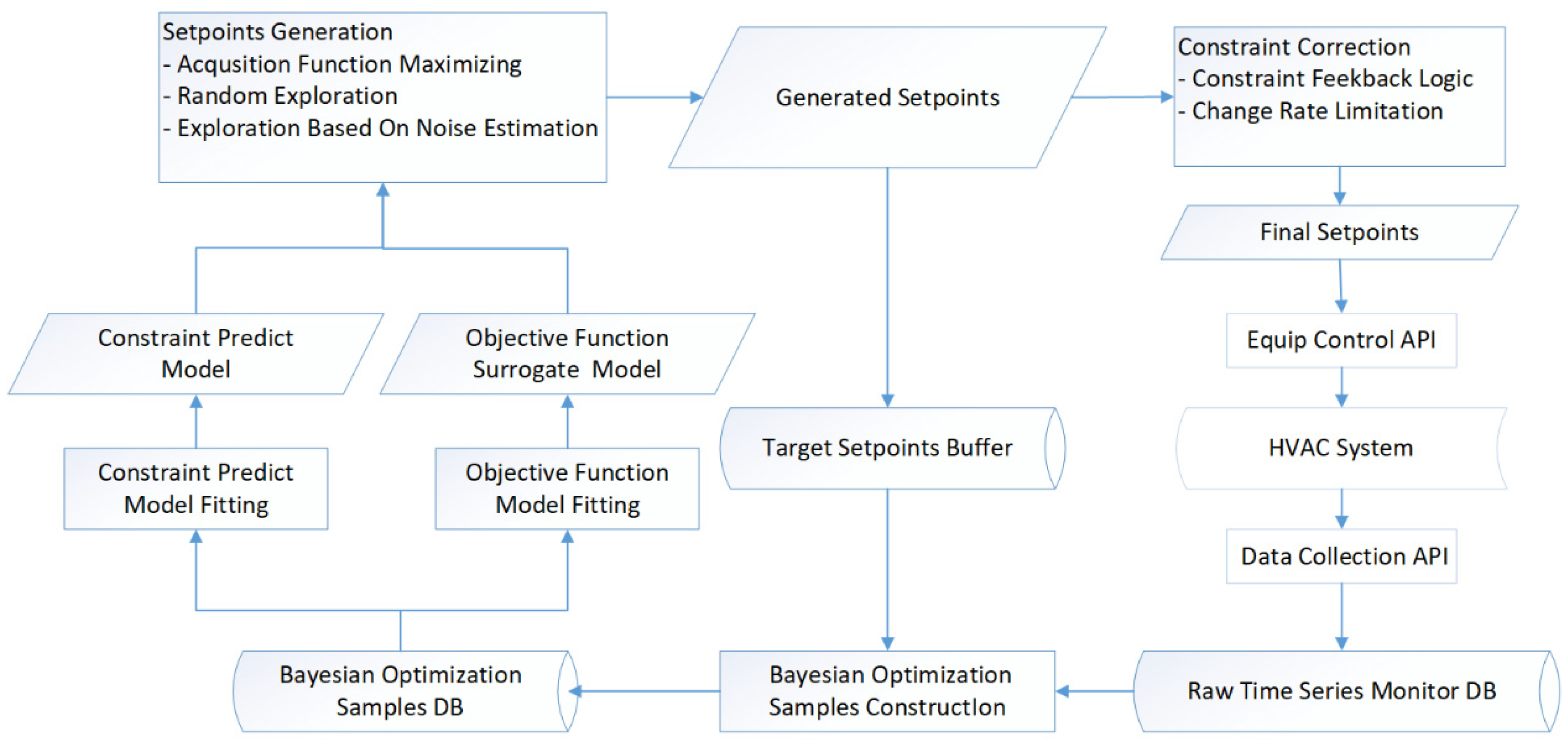Figure 1 shows the overall Bayesian optimization framework for HVAC control.

Starting from a physical HVAC system, the main Bayesian optimization control loop included the following steps:

• We collected trending data for HVAC systems by using a data collection application programming interface (API) from the Internet of Things (IoT) platform. Next, we conducted some preprocessing and stored the results in a raw time series database. A few of the common preprocessing activities include the following.

• The timestamp alignment of different sensor points simplify the subsequent use of monitor data, which is usually aligned to one sample per minute.
• The useful virtual points calculated by the raw sensor points, such as the total power of the whole HVAC system, the average indoor air temperature and the quantity of running chillers, are added.
• The data calibration and abnormal warning of sensor data are carried out.

2

We constructed Bayesian optimization samples from the raw time series database and stored the results in a Bayesian optimization sample database. This was implemented by aggregating a period of raw time series data into one aggregated sample. The last generated setpoints were used to build the Bayesian optimization samples. However, the generated setpoints were modified by the subsequent constraint correction. Therefore, the generated setpoints could not be reconstructed from the raw time series monitor database. Instead, an additional target setpoint buffer was used to store the setpoints that were historically generated. In Section 4, we describe the sample construction process in more detail.

3

The Bayesian optimization sample database was used to fit the surrogate model of the objective function and the prediction model of the constraints. In Section 5, we explain the objective function modeling, and in Section 6.2, we explain the constraint processing.

4

We generated the best setpoints corresponding to the current objective function surrogate model by constraint optimizing the acquisition function of Bayesian optimization. To make Bayesian optimization more robust in terms of noise observation, we used additional random exploration and noise-based exploration. In Section 6, we demonstrate the details of the setpoints’ generation.

5

We corrected the generated setpoints by predefining the constraint condition to ensure that the setpoints were safe for HVAC system operations. Next, we applied the final setpoints to the HVAC system control by mapping API from the IoT platform. The feedforward constraint optimization in Step 4 and the feedback constraint correction here provided a dual guarantee of the HVAC system’s operational safety. In Section 6.2, we will demonstrate the details of this.

4. The Construction of the Bayesian Optimization Samples

This section introduces the process that we used to construct the Bayesian optimization samples from the raw time series trending data. This section is organized as follows: In Section 4.1, we describe the main idea behind modeling the HVAC control problem as a contextual optimization problem. We also describe the main process that we used to construct the Bayesian optimization samples. In Section 4.2, we describe the main transition characteristics that we used when we adjusted the setpoints and the algorithm to automatically identify the end time of the transition process. This was used to exclude the transition process when we aggregated the Bayesian optimization samples. In Section 4.3, we describe our method for deciding whether the observation of current setpoints should be continued. This method was used to obtain the Bayesian optimization samples that could represent the real performance. In Section 4.4, we describe the main fields and methods of data aggregating that we used to construct the Bayesian optimization samples.

4.1. Main Idea

The goal of an HVAC system is to control space temperature and humidity, keeping them within a certain range. Other parameters also change over time, e.g., the flow rate; the pressure and temperature of the chilled and cooling water; and the outlet air temperature of AHUs. Once the range of the space’s temperature and humidity can be successfully controlled, the other parameters can be optimized to achieve better energy efficiency.

Using Bayesian optimization to control the space temperature and humidity directly is very difficult because the space temperature and the humidity need real-time and stable dynamic control, but Bayesian optimization is unable to handle the dynamic closed-loop control of an HVAC system. Typically, an air system is controlled by using a traditional BA sequence to control the space temperature and humidity. However, by utilizing the thermal capacity of the system, the setpoints of the water system can be adjusted within a relatively large range without making the space temperature and humidity exceed the required range. Therefore, it is practical to use Bayesian optimization to optimize the setpoints of water systems. Because the BA setpoints usually use quasistatic values, which are set according to an engineering judgment, the hour-long adjustment interval of the setpoints used in Bayesian optimization is sufficient to produce a significant energy-efficiency improvement compared with BA controls.

To enable Bayesian optimization for HVAC controls, the energy efficiency of certain setpoint values, under certain contextual values, should be obtained, which is denoted by $\mathrm{r}\left(s,a\right)$. Here, $s$ stands for contextual values, and $a$ stands for setpoint values. The trending data of HVAC systems are usually in minute-long time steps; however, constructing $\mathrm{r}\left(s,a\right)$ directly in this interval is not practical, owing to the high noise, high randomness and high proportion of the transition time. Therefore, they cannot represent the actual stable performance of the setpoints. Thus, $\mathrm{r}\left(s,a\right)$ is constructed by properly aggregating the time series data.

Algorithm 2 shows the pseudocode for collecting one $\mathrm{r}\left(s,a\right)$ sample from an interaction with an HVAC system. The main logic is explained, as follows: When applying new desired setpoints $targetSP$ to HVAC systems at a certain time stamp $t_0$ to obtain $\mathrm{r}\left(s,targetSP\right)$, it takes a while for the HVAC system to complete the transition process, owing to the setpoint adjustment. Here, $t_s$ is used to denote the end time of the transition process. The HVAC systems’ performance is then observed under this desired $targetSP$ for a sufficient duration to construct the $\mathrm{r}\left(s,targetSP\right)$, which is then stored in the database (bayesDB). The Bayesian optimization control loop will then use this bayesDB to fit the surrogate model for the objective function and to generate a new $targetSP$.

Algorithm 2: Pseudocode of construct for one Bayesian optimization sample from the raw time series monitor data

1: def collectOneSample(${\mathit{t}}_0$, targetSP, minTransConformDuration, 2: minBayesObsDuration, maxBayesObsDuration, maxDuration): 3: while t < $t_0$ + minTransConformDuration: 4:  monitorHVAC() 5: $t_s$ = getEndOfTransTime($t_0$, t) 6: while$t_s$ is None and t < $t_0$ + maxDuration-minBayesObsDuration: 7:  monitorHVAC() 8:  $t_s$ = getEndOfTransTime($t_0$, t) 9: if $t_s$ is None: 10:  finishTrans = False 11:  $t_s$ = t 12: else: 13:  finishTrans = True 14: while (t < $t_s$ + minBayesObsDuration) or ((t < min($t_s$ + maxBayesObsDuration, $t_0$ + maxDuration) and continueBayesObs($t_s$, t)): 15:  monitorHVAC()transDB <- transDB ∪ aggTransData($t_0$, $t_s$, finishTrans, targetSP) 16:  bayesDB <- bayesDB ∪ aggBayesData($t_s$, t, finishTrans, targetSP)

For details on minTransConformDuration, maxDuration and getEndOfTransTime, refer to Section 4.2. For details on minBayesObsDuration, maxBayesObsDuration, continueBayesObs, refer to Section 4.3. For details of aggTransData and aggBayesData, refer to Section 4.4.

4.2. Transition Process Identification

The period of the transition process during the setpoint adjustment of an HVAC system is identified and excluded when constructing $\mathrm{r}\left(s,targetSP\right)$. In the exploration process of the Bayesian optimization, the next $targetSP$ that is generated may be very different from the existing setpoints, which results in drastic changes in the short-term performance of the transition process. However, when the exploration has been completed and the system operates in the stable optimal control stage, the variation in $targetSP$ will be relatively small and the drastic changes in the performance will not happen; therefore, the performance of the transition process in the exploration process should not be taken into account when constructing $\mathrm{r}\left(s,targetSP\right)$.

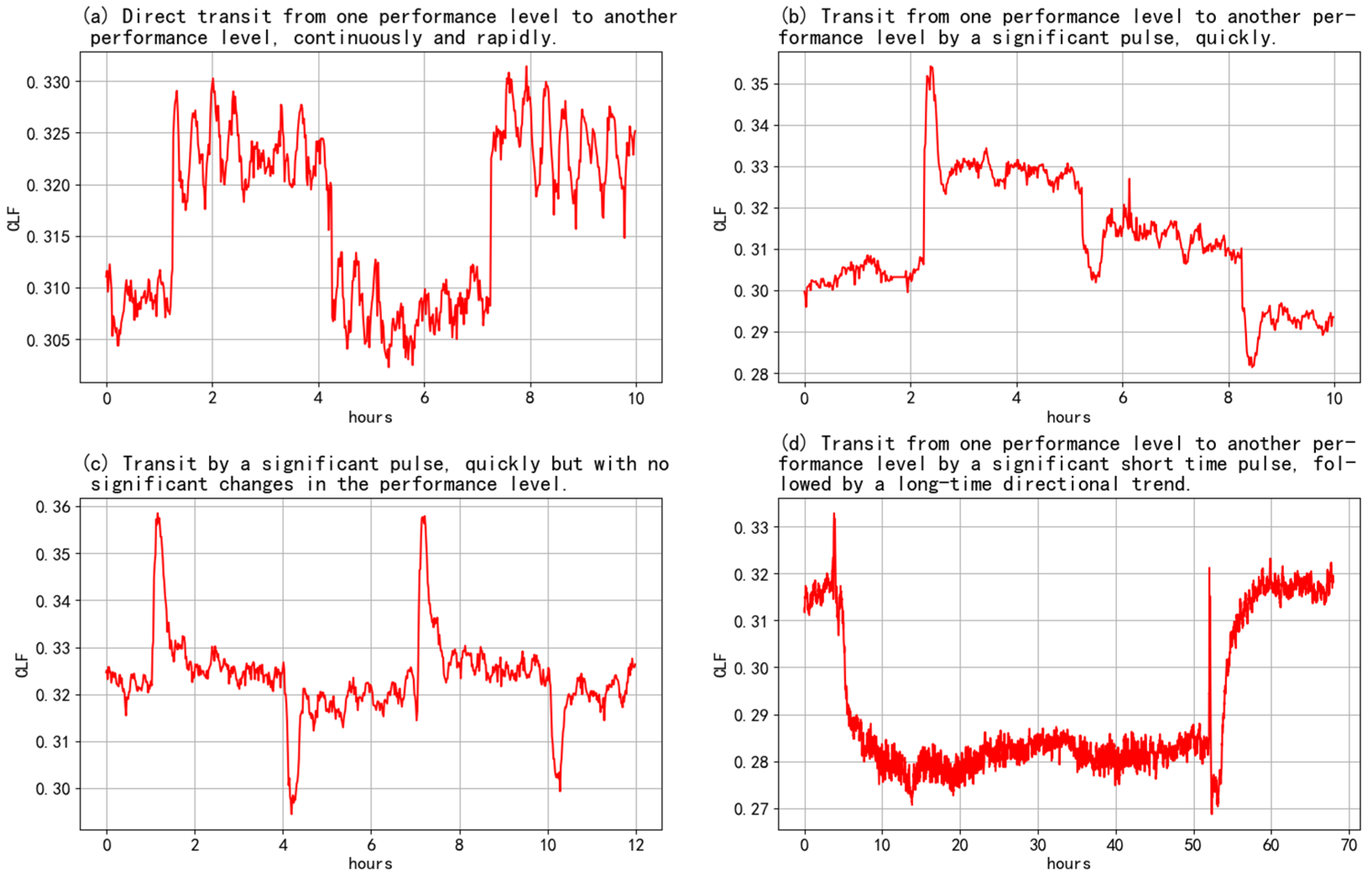
In this study, by observing the online system transition tests, we were able to summarize the four main transition period types (shown in Figure 2): type (a) demonstrates the direct transit from one performance level to another performance level, continuously and rapidly; type (b) demonstrates the transit from one performance level to another performance level by a significant pulse, quickly; type (c) demonstrates the transit by a significant pulse, quickly but with no significant changes in the performance level; and type (d) demonstrates the transit from one performance level to another performance level by a significant short time pulse, followed by a long-time directional trend. In some cases, no significant transition process existed, and these cases have not been included in these four categories. The goal of this transition process identification was to automatically identify these types of transition processes and to keep the correct prediction when no significant transition process existed.

Because the start time of a transition process was equal to the adjustment time of the setpoints, only the end time of the transition process needed to be predicted. As can be seen in Figure 2, the dynamic characteristics of the original objective function value were complex. These included the trends in both directions and the significant fluctuations that occurred even outside of the transition process period. However, we observed that the standard deviation of the objective function value was always larger in the transition process; thus, the standard deviation could be used to easily identify the transition process. In addition, because the standard deviation was not sensitive to the slow trend of the objective value, the trend detection after the standard deviation detection could be combined to complete the identification. A front standard deviation detection was used to deal with the situation in which no significant transition process existed. Algorithm 3 shows the pseudocode of the whole identification process, which returns the end time of the transition process or which returns ‘None’ when the transition process has not yet ended. Here, $t_b$ and $t_e$ are set by Algorithm 2.

Algorithm 3: The pseudocode of the transition process identification

1: def getEndOfTransTime($t_b$, $t_e$, window = 30 min, stdDecayThreshold = 0.2, objectiveTrendThreshold = 0.03): 2:  data = read raw time series monitor data between $t_b$ − 2 * window to $t_e$ from DB 3:  lowpassObjective = low-pass filtering of objective function value by butterworth filter with order = 4 and critical frequency = 0.2 [17] 4:  lowpassObjectiveMovingStd = rolling standard deviation of lowpassObjective with the specified window length and center = True 5:  if maximum value of lowpassObjectiveMovingStd between $t_b$ and $t_b$ + window less then 2 * maximum value of lowpassObjectiveMovingStd between $t_b$ − window and $t_b$ − window/2: 6:   return$t_b$ 7:  maxStd, minStd = maximum and minimum value of lowpassObjectiveMovingStd between $t_b$ and $t_e$ 8:  stdThreshold = (maxStd − minStd) * stdDecayThreshold + minStd 9:  t1 = find the time of the maximum value of lowpassObjectiveMovingStd between$t_b$ and $t_e$ 10:  t2 = find the first time when lowpassObjectiveMovingStd lower than stdThreshold after t1 11:  t3 = find the first time of local minimum of lowpassObjectiveMovingStd after t2 12:  $t_s$ = t3 − window/2 13:  lowpassObjective2 = low-pass filtering of objective function value between $t_s$ and $t_e$ by butterworth filter with order = 4 and critical frequency = 0.02 14:  ratio = (lowpassObjective2.max() − lowpassObjective2.min())/lowpassObjective2.min() 15:  if ratio > objectiveTrendThreshold: 16:   objectiveTrend = moving diff of lowpassObjective2 with periods = -window/2 17:   t4 = find the last time when objectiveTrend greater than 0.01 * (lowpassObjective2.max() − lowpassObjective2.min()) 18:   if t4 is the last valid time of objectiveTrend, thus means still in transition trend: 19:    $t_s$ = None 20:   else: 21:    $t_s$ = t4 + 1 22:   return$t_s$

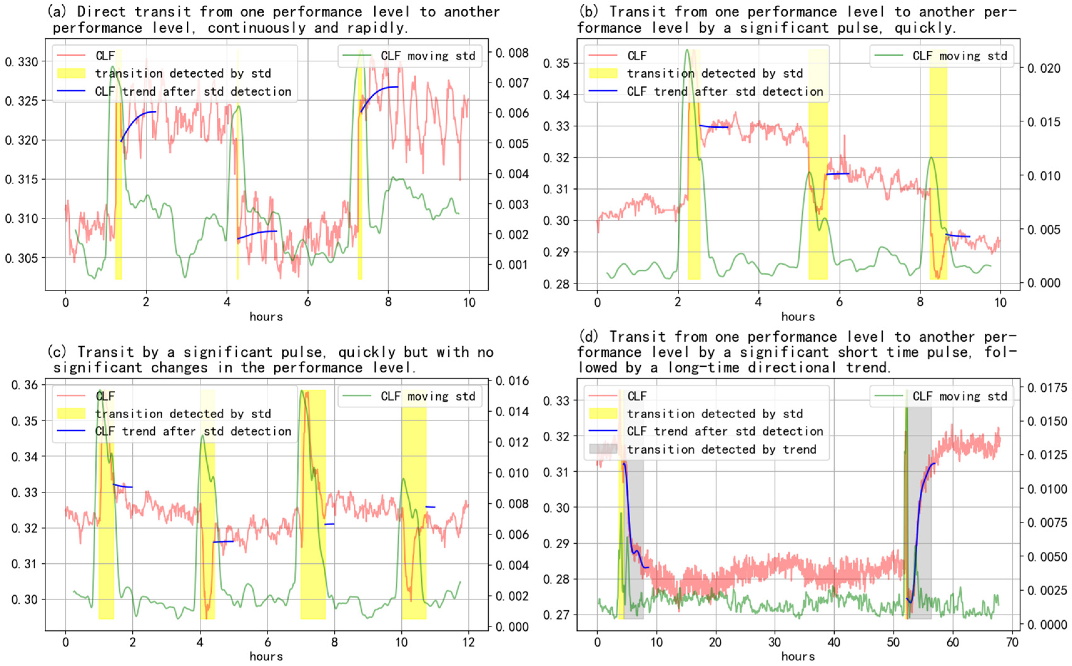
There are two low-pass filterings in Algorithm 3. The first filtering is used mainly to eliminate the outliers of the objective function to obtain a smooth standard deviation estimate and, thus, to use a high critical frequency. The second filtering is used mainly to eliminate the fluctuation of the objective function to obtain the trend part and, thus, to use a low critical frequency. In our test, most of the differences between the identified transition durations and the manual labels were within 10%. The images in Figure 3a–d were selected as examples from the different time periods in which the transient processes occurred. The images in Figure 3a–c show the transient processes only with dramatic parameter changes (e.g., VFD speed reset), which can be detected with a standard deviation estimation. The yellow areas of these figures show the transient periods. The image in Figure 3d shows the transient process with a low trend (e.g., chilled water temperature reset), in which the trend detection and the standard deviation detection were combined to complete the identification. The trend detection period is demonstrated through the gray areas.

4.3. Bayesian Observation Duration Decision

In this study, Bayesian observation meant observing the performance of the HVAC system for a period of time to construct the $\mathrm{r}\left(s,targetSP\right)$ sample for the Bayesian optimization. The duration of the Bayesian observation needed to be balanced. If the duration of the observation had been insufficient, the observed performance would have been with high noise owing to various random factors or with high bias owing to only a small part of the performance oscillation period’s being observed. However, if the duration of the observation had been too long, the optimization would have been slowed down and the state during the observation may have been too far away from the initial state.

To obtain a proper duration of the observation, the duration was limited to between minBayesObsDuration and maxBayesObsDuration, where minBayesObsDuration and maxBayesObsDuration were the hyperparameters set by an engineering judgment—usually 30 min for minBayesObsDuration and 3 h for maxBayesObsDuration. Next, continueBayesObs was used to decide whether to continue the observation between minBayesObsDuration and maxBayesObsDuration. This returned the response ‘True’ only when it needed to continue the observation, which would have been the case in the following situations:

• In performance changes in which a significant trend was detected by a trend detection algorithm, similar to Algorithm 3.
• If the feedback constraint correction was triggered, as judged directly by the feedback correction log.

4.4. Data Aggregation

After finishing the transition process and the Bayesian observation process to obtain the $targetSP$, the aggregated transition data sample and the Bayesian data sample were constructed into the transDB and bayesDB, respectively.

An $aggTransData$ was used to aggregate the transition data. Because the transition process data were not used directly for optimization, the $\left(sampleId,t_0, t_s, finishTrans, targetSP, duration=t_s-t_0\right)$ tuple was returned for log purposes, where sampleId was the unique identifier of one call to collectOneSample.

An aggBayesData was used to aggregate the Bayesian observation data; the $\left(sampleId, t_s, t, finishTrans, targetSP, duration=t-t_s,s, reward, exceedConstraint, noise, infos, resampleCount=0\right)$ tuple was returned for optimization purposes, where the sampleId was the same as it was in the aggTransData; and the remaining fields were constructed as follows:

• The $s$ was constructed by averaging the state variables between the timestamp, as follows: ${\mathrm{t}}_{\mathrm{s}}- \mathrm{T}$ and ${\mathrm{t}}_{\mathrm{s}}$, where $\mathrm{T}$ is the hyperparameter of time length (usually 15 min, in practice).
• The $reward$ was constructed by averaging the performance variable so that it could be optimized between timestamp ${\mathrm{t}}_{\mathrm{s}}$ and $\mathrm{t}$. Note that $\mathrm{reward} = \mathrm{r}\left(\mathit{s},\mathit{a}\right)=\mathrm{r}\left(s,targetSP\right)$ formed the Bayesian optimization samples.
• $exceedConstraint$ is a bool variable indicating whether the space temperature limit has been exceeded and is used to support constraint optimization. The constraint judgment conditions in this study were manually predefined. When the temperature limit was greatly exceeded for a long time, the constraint was considered to be violated and exceedConstraint was set to ‘True’.
• The word ‘noise’ represents the noise estimate of the reward and was used to support better exploration, based on the noise in optimization. However, noise does not represent the fluctuation of the original objective function but rather the uncertainty of the aggregated reward. The noise was designed to be high when the finishTrans was ‘False’ or the objective function value had an unfinished trend.
• The infos was constructed by averaging the useful trended points of an HVAC system between the timestamp (${\mathrm{t}}_{\mathrm{s}}$) and $\mathrm{t}$ for potential debugging and algorithm upgrade purposes.
• The resampleCount was initialized to zero and was used to record the resample times of this targetSP in the optimization loop.

5. Surrogate Model for Objective Function

Once the Bayesian optimization samples had been obtained, they could be fitted by using a surrogate model. After this, the model was used to predict the objective function value in the Bayesian optimization loop. The Gaussian process regression model was selected as the surrogate model thanks to its excellent probability prediction properties. Because the mean function of the Gaussian process is usually set as a constant value, a kernel function was designed.

By following the common forms in Bayesian optimization, the optimization problem was expressed as a maximization problem; thus, the negative total power of the whole HVAC system was used as an objective function value. The feature variables of the surrogate model included the following three categories:

• Device power-on status—an HVAC water system may include multiple parallel devices, such as chillers and pumps. The actual power-on devices will change over time. Because different parallel devices may have significantly different energy efficiency, the power-on status of the devices needs to be a part of the model’s features. Another approach could be to simply use the quantity of parallel power-on devices to replace the detailed power-on status when the parallel device’s model and pipe connection are similar to reduce the model’s complexity.
• Setpoints—setpoints are the variables to be optimized in an HVAC water system. They include the chilled water outlet temperature of the chillers and the frequency of the water pumps and cooling tower fans, in the form of float numbers.
• Environment variables—environment variables may have a significant impact on the energy efficiency of an HVAC system, such as the IT load of the data center and the outdoor wet bulb temperature. Because the Gaussian process and Bayesian optimization find it difficult to deal with high-dimensional features, typically only a small number of key environment variables are added to the features.

Through our test, it was found that setpoints and environment variables can be mixed without affecting the model’s performance. It was also found that the best way to deal with the device power-on status was to use different independent submodels for different power-on statuses. Although using a multitask Gaussian process model and a multitask Bayesian optimization to deal with mixed power-on status data is a possible approach that could be used to improve the optimization efficiency [13], as we had not achieved the expected test results at this point, we chose to use independent submodels in this study. However, upgrading to multitask Bayesian optimization will not affect the structure of the proposed framework.

LinearKernel and MaternKernel [16] were selected as the kernel functions for the setpoints and the environment variables. The LinearKernel was used to deal with the overall trend, and it was useful in extrapolating the prediction. The MaternKernel was used to deal with the complex nonlinear relation.

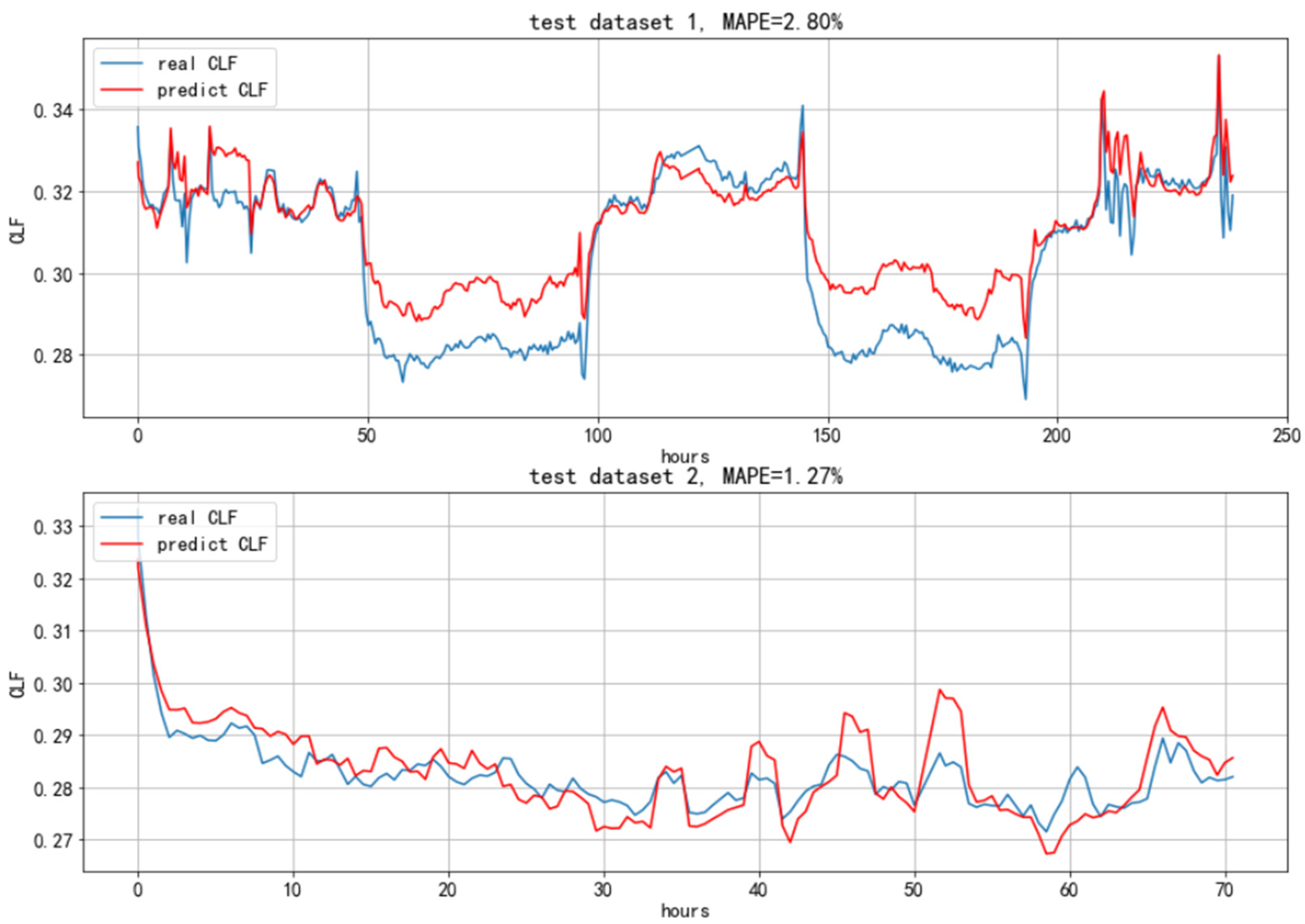
Figure 4 shows the prediction results from the test sets of two data sets from a data center. In this case, the setpoints included the outlet water temperature of the chillers, the frequency of the cooling tower fans, the cooling pumps and the primary and secondary chilled pumps. The environment variables included the IT load of the tested data center, the outdoor wet bulb temperature and the chiller load factors. Data sets 1 and 2 were divided by the chiller’s power-on status. The data were modeled by two submodels, and the respective mean absolute percentage errors of the test sets were 2.8% and 1.27%. As a comparison, the respective test errors of the linear regression model were 4.88% and 1.69%, and for the lightGBM model, the respective test errors were 6.33% and 2.31%. In order to evaluate the performance of the extrapolation prediction, the time between the selected training set was far away from the test set. The training set of data set 1 was 1 month before the test set, and the training set of data set 2 was 1 week before the test set.

6. Bayesian Optimization Control Loop

Algorithm 4 introduces the basic Bayesian optimization control loop for HVAC systems. It is similar to the standard Bayesian optimization process in Algorithm 1, except that UCB is directly used instead of a general acquisition function. UCB is defined as $mean+alpha·std$, where $alpha$ is the exploration coefficient, which is usually set to constant two.

Algorithm 4: Basic process of Bayesian optimization control loop for HVAC systems

1: initial: transDB <- ∅, bayesDB <- ∅, setpoints $\mathit{S}\mathit{P}$, surrogate model for objective function $reward=GP\left(\mathit{s}, \mathit{a}\right)$, minTransConformDuration, minBayesObsDuration, maxBayesObsDuration, maxSampleDuration 2: logic: 3: $\mathit{i}\mathit{n}\mathit{i}\mathit{t}\mathit{S}\mathit{P}$ = randomSampleSP() 4: sendToHVAC($\mathit{i}\mathit{n}\mathit{i}\mathit{t}\mathit{S}\mathit{P}$) 5: collectOneSample(now(), $\mathit{i}\mathit{n}\mathit{i}\mathit{t}\mathit{S}\mathit{P}$, minTransConformDuration, minBayesObsDuration, maxBayesObsDuration, maxSampleDuration) 6: while True: 7: $GP$ = fitGPModel(bayesDB) 8: $\mathit{S}{\mathit{P}}^{* }=\underset{\mathit{S}\mathit{P}}{arg max}UCB\left(GP\left(currentState(),\mathit{S}\mathit{P}\right)\right)$ 9: sendToHVAC($\mathit{S}{\mathit{P}}^{*}$) 10: collectOneSample(now(),$\mathit{S}{\mathit{P}}^{*}$, minTransConformDuration, minBayesObsDuration, maxBayesObsDuration, maxSampleDuration)

Both transDB and bayesDB were initialized to be empty and were set to hold the transition data and the Bayesian optimization sample data, respectively. SP stands for all the setpoints to be optimized; minTransConformDuration, minBayesObsDuration, maxBayesObsDuration and maxSampleDuration are hyperparameters of the sample duration (described in Section 4); randomSampleSP represents the random sampling of one SP within the configured bounds, uniformly; sendToHVAC represents the application of the selected SP to the HVAC system control by a device-controlled API; collectOneSample represents the collection of one Bayesian optimization sample (described in Section 4); currentState represents the calculation of the current state, according to the method of constructing state properties in bayesDB; and fitGPModel represents the fitting of the surrogate model for the objective function reward GP(s,a) with the newest bayesDB data.

We chose UCB as an acquisition function because the best settings for HVAC controls are generated continuously online—unlike in the common Bayesian optimization scenarios, in which the goal is to find better settings within a given number of trials. As we expected, after sufficient explorations, UCB was able to generate the candidates with the maximum performance; however, other acquisition functions, such as EI, may generate only random candidates because the acquisition function value cannot be improved any more.

The following subsections describe how we dealt with the noise observation problem and the constraint guarantee problem in HVAC controls.

6.1. Noise Observation

The constructed Bayesian optimization samples contained noise owing to the original observation noise in the HVAC system or the aggregation bias. The noise may damage the optimization process because of the use of possible wrong rewards to guide the optimization. In addition to the original sensor calibration, which is important in engineering applications but not covered in this paper, some other tricks were used in the candidate generation to make the optimization more robust in terms of noise observation and, thus, more likely to find the global optimal setpoints, as shown in Algorithm 5.

Algorithm 5: Pseudocode to generate the next setpoints, as the in-place replacement of the $argmax$ line in Algorithm 4

1: initial: ${\mathsf{\alpha }}_0$, ${\mathsf{\beta }}_0$ 2: def generateNextSP(GP): 3: ${\mathsf{\alpha }}_t={\mathsf{\alpha }}_0 \mathit{d}\mathit{e}\mathit{c}\mathit{a}\mathit{y} \mathit{b}\mathit{y} \mathit{t}$ 4: ${\mathsf{\beta }}_{\mathit{t}}={\mathsf{\beta }}_0 \mathit{d}\mathit{e}\mathit{c}\mathit{a}\mathit{y} \mathit{b}\mathit{y} \mathit{t}$ 5: rnd = uniform(0, 1) 6: if rnd < ${\mathsf{\alpha }}_t$: 7:  $\mathit{S}{\mathit{P}}^{* }$= randomSampleSP() 8: elif rnd < ${\mathsf{\alpha }}_{\mathit{t}}$ + ${\mathsf{\beta }}_{\mathit{t}}$: 9:  $\mathit{S}{\mathit{P}}^{* }$= resample from bayesDB whih low resampleCount and high noise 10: else: 11:  $\mathit{S}{\mathit{P}}^{* }$= $\underset{\mathit{S}\mathit{P}}{\mathit{a}\mathit{r}\mathit{g} \mathit{m}\mathit{a}\mathit{x}}\mathit{U}\mathit{C}\mathit{B}\left(\mathit{G}\mathit{P}\left(\mathit{c}\mathit{u}\mathit{r}\mathit{r}\mathit{e}\mathit{n}\mathit{t}\mathit{S}\mathit{t}\mathit{a}\mathit{t}\mathit{e}(),\mathit{S}\mathit{P}\right)\right)$ 12: return $\mathit{S}{\mathit{P}}^{* }$

A certain probability was reserved to perform the random sampling or resampling of the setpoints with high reward estimation noise, which were executed. The random sampling probability decreases with time; therefore, an initial sample probability and a probability decay form were set for the system on the basis of an engineering judgment.

6.2. Constraint Guarantee

A combination of feedforward constraint optimization and feedback constraint correction were used to ensure the constraint conditions in the Bayesian optimization control loop. Feedforward constraint optimization involves using a constraint prediction model to estimate whether any setpoints will cause the HVAC system to break through the constraint conditions when generating the next setpoints. In this study, we selected setpoints that kept the constraint conditions and maximized the acquisition function, simultaneously. Feedback constraint correction involves monitoring the constraint conditions online. When the constraint conditions are broken, the predefined feedback correction logic is used to modify the setpoints generated by the optimization algorithm and to apply the modified setpoints to system control.

Algorithm 6 shows the main logic of feedback constraint correction. Because of system differences, in this study the feedback constraint correction rule was manually specified for each system, as a plugin of the framework.

Algorithm 6: The main logic of feedback constraint correction

1: initial: rule table for adjust direction and step size of each setpoint when each constraint condition is broken. 2: def constraintCorrection(generatedSetpoints): 3:  do constraint conditions detection for last time window 4:  if all constraint conditions are satisfied: 5:   return generatedSetpoints 6:  for each broken constraint condition: 7:   for each setpoint in rule table of current broken constraint condition: 8:    lastValue =average feedback value of current setpoint of last time window 9:    if adjust direction is increase: 10:     minValue = lastValue + step size * amplitude of constraint broken 11:     generatedSetpoints[current setpoint] = max(generatedSetpoints[current setpoint],minValue) 12:    else: 13:     maxValue = lastValue − step size * amplitude of constraint broken 14:     generatedSetpoints[current setpoint] = min(generatedSetpoints[current setpoint], maxValue) 15:  return generatedSetpoints

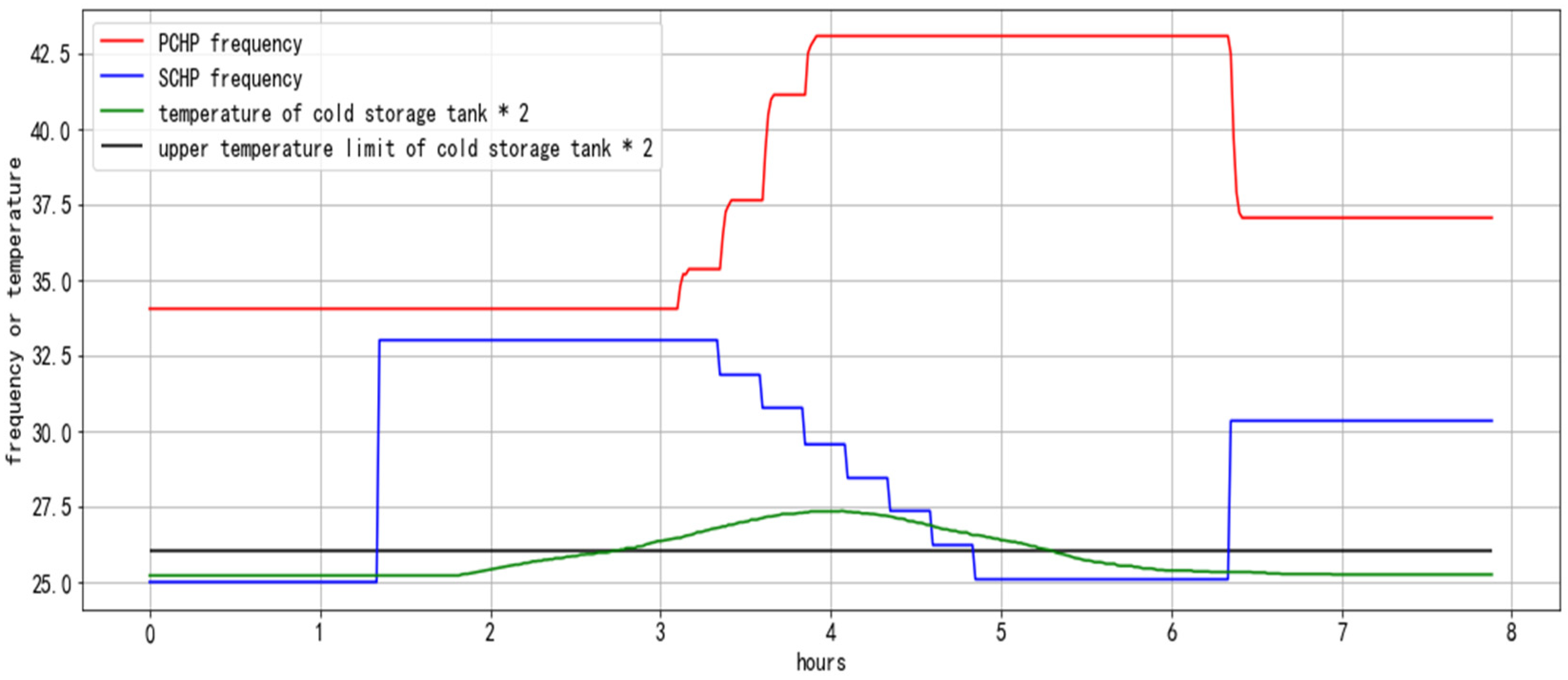
Figure 5 shows an online feedback constraint correction process for the temperature of cold storage tanks in a data center. The correction rule is that when the temperature of a cold storage tank is higher than the predefined threshold, the frequency of the primary chilled pumps should be increased and the frequency of the secondary chilled pumps should be decreased.

For a feedforward constraint optimization, binary classification models for constraints are fitted after every new sample collection. Next, a genetic algorithm is used to maximize the acquisition function, under the constraints given by the fitted constraint models; i.e., a listener function is registered into the genetic algorithm search process. When a solution in the population violates the constraint, the solutions most similar to Algorithm 6 must be collected until the constraint has been met, and then this modified solution is used in the subsequent search process. When there is no solution that meets the constraints, a predefined limit value is used.

7. Results

In this study, the performance of the Bayesian optimization framework was tested on a simulated HVAC system of a data center. The model of this HVAC system was calibrated with real trending data. The HVAC system of the data center contained five chillers and corresponding cooling towers; cooling pumps, primary chilled pumps and secondary chilled pumps in its water system; and approximately 10 IDC rooms and more than 100 air-conditioning terminals in its air system. The chillers rotated their order every week, and the constraints included that the temperature of the IDC room be lower than 25 °C and that the temperature of the cold storage tank be lower than 13 °C.

Substantial tests were conducted on this HVAC system to obtain the dynamic characteristics of the system before starting this Bayesian optimization framework study. Because it was difficult to simulate the transition process and the constraint correction process of the system with high precision and because these processes are relatively independent of the Bayesian optimization logic and performance, we verified the algorithms to process these processes by using only historical data, as shown in Figure 3 and Figure 5. Nevertheless, the Bayesian optimization performance on the simulated energy-efficiency model was validated by the historical data, and an additional transition duration prediction model was fitted by the historical data to help with the evaluation of the optimization duration, the simulated setpoints and environment variables, which can be referred to in Section 5.

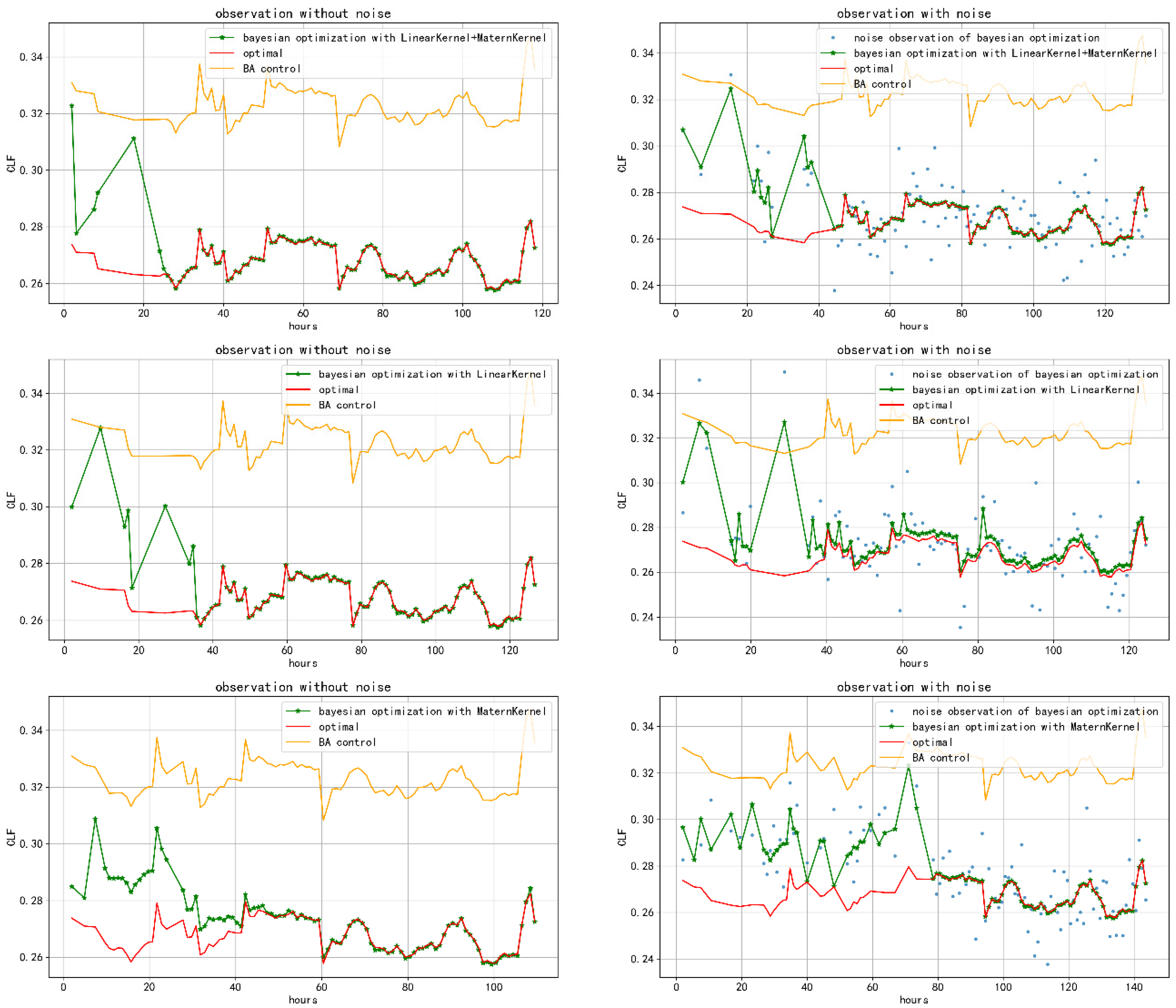
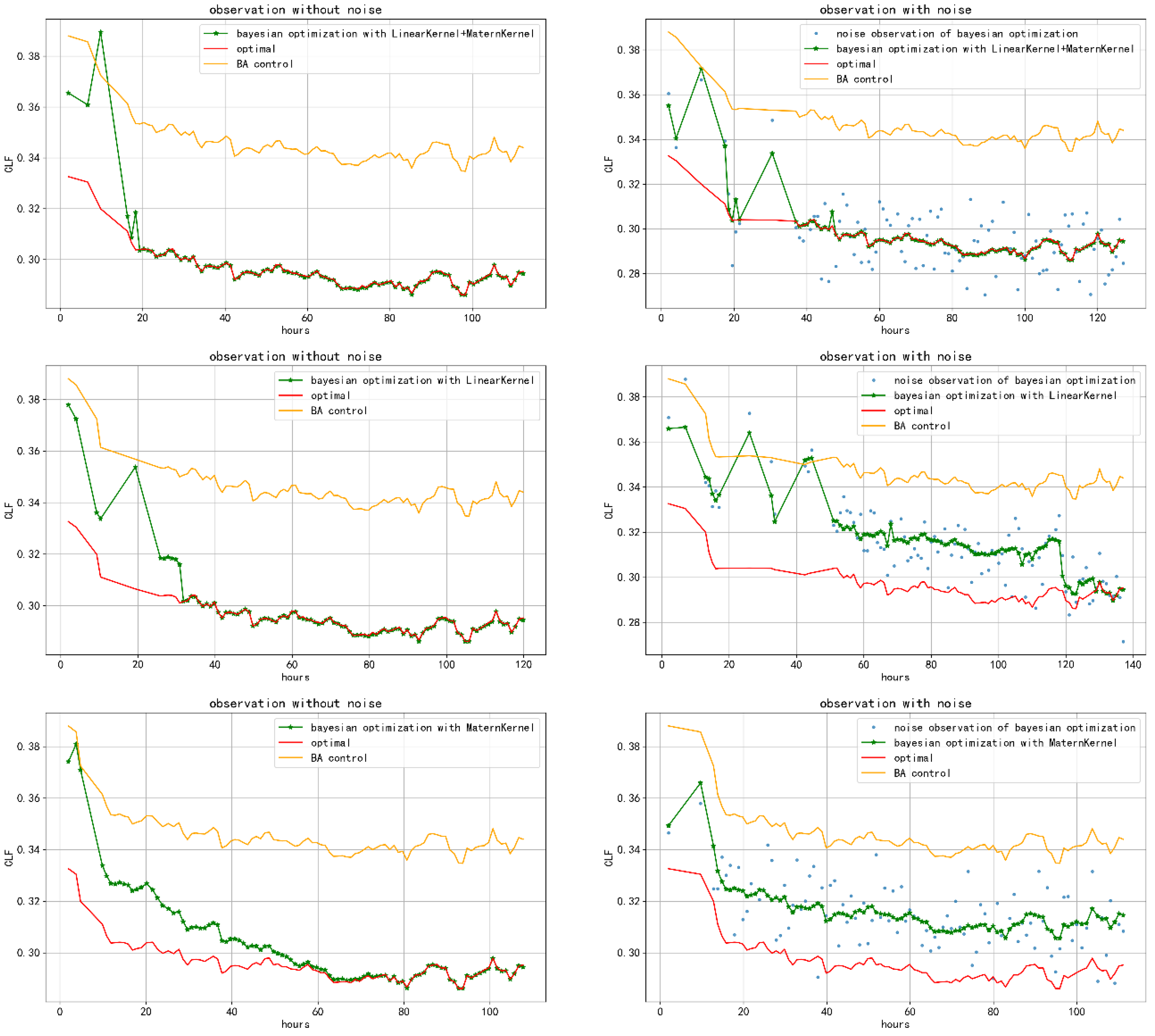
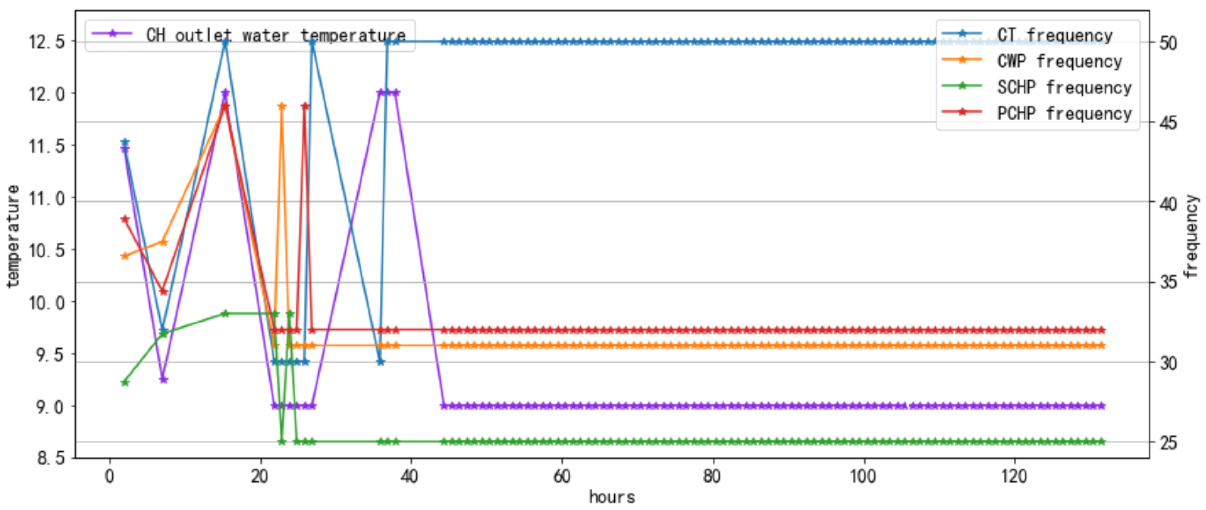
Figure 6 and Figure 7 show the energy efficiency of the optimization process for the different algorithm configurations on two sets of power-on chillers, respectively. ‘BA control’ in the legend stands for the cooling load factor (CLF), which was predicted by the setpoints of BA logic in the current environment. ‘Optimal’ in the legend stands for the optimal CLF under the current environment. Figure 8 shows the setpoint variation process, which corresponds to the upper-right Bayesian optimization process, shown in Figure 6.

We summarize our test conclusions as follows:

• With proper LinearKernel + MaternKernel models, we were able to obtain the optimal setpoints in 50 h of training, even though there were significant observation noises. The control approach achieved an energy-efficiency improvement of more than 10% compared with the BA controls. This proves the efficiency of Bayesian optimization.
• Some optimal setpoints in this simulation system did not change with the environment. The main reason for this was that the optimal setpoint was on the boundary of the configured setpoint range; thus, they will not change. This proves that Bayesian optimization can continuously generate stable optimal setpoints for the current model.
• When there are significant observation noises, the optimization process will slow down. The optimal solution cannot be obtained on some bad kernel functions; therefore, a proper kernel function design is crucial to the Bayesian optimization process.

8. Conclusions

This paper proposed a Bayesian optimization framework for HVAC controls, which aimed to optimize the setpoints of the water system to achieve high energy efficiency. In this study, historical data testing and simulation experiments proved its feasibility and effectiveness. The main advantages of the proposed Bayesian optimization framework for HVAC controls are as follows:

• High efficiency—by taking advantage of the Bayesian optimization technology, we can achieve near-optimal control performance within a few weeks.
• Safety—thanks to the combination of feedforward constraint optimization and feedback constraint correction, the operation safety of the implemented HVAC system can be fully guaranteed.
• Stability—because of the simple form of the Gaussian process regression surrogate model and of the UCB acquisition function, no complex parameters need to be adjusted. Unlike reinforcement learning, the model is not affected by random noises; therefore, we can achieve stable performances across systems and times.
• Easy to deploy—the main configurations that need to be customized for different HVAC systems are the feedback correction rules, which are usually easy for HVAC system operation engineers to implement. Furthermore, the rules for common system types can be predefined in the framework.

In future studies, we will verify the effectiveness of the complete framework in more HVAC systems. In addition, we will make more system configurations that can be automatically completed, to reduce the cost and threshold of the framework’s deployment.