Enhancing the Vulnerability Assessment of Rainwater Pipe Networks: An Advanced Fuzzy Borda Combination Evaluation Approach

Abstract

A vulnerability assessment system for rainwater pipe networks, comprising 13 indexes, was developed to facilitate the rational allocation and timely updating of urban storm drainage systems. An enhanced Borda combination evaluation method, which considers both the optimal and worst solutions, was proposed, accompanied by the operation procedure and numerical calculation method. Five stormwater systems in Central China were selected as case studies, and their vulnerability was evaluated and compared using five distinct evaluation methods: the entropy weight method, the Technique for Order Preference by Similarity to an Ideal Solution (TOPSIS), the efficacy coefficient method, the fuzzy comprehensive evaluation method, and the improved fuzzy Borda combination evaluation method. The results demonstrated that the correlation coefficients between the fuzzy Borda combination evaluation method and the four individual evaluation methods were equal to or greater than 0.88, indicating strong agreement. Additionally, the compatibility of the combination evaluation method was found to be 0.96. This study holds both theoretical significance and practical value for preventing urban waterlogging and contributes to the development of more resilient urban storm drainage systems.

1. Introduction

Urban infrastructure systems have become increasingly vulnerable due to the frequent occurrence of extreme natural events [1,2,3]. Rainstorm waterlogging, caused by extreme climate change, has gradually drawn attention from researchers and policymakers [4,5,6]. The drainage pipe network is one of the most critical sectors in this context, and a systematic evaluation of the rainwater pipe network is necessary to identify vulnerable pipes, considering the complexity of the system. The research objective of this study is to evaluate the vulnerability of urban rainwater pipe networks and identify weak pipe sections to determine the corresponding vulnerability levels of the system. This information can provide forecasting plans and data support for urban waterlogging emergency management departments [7,8].

Numerous experts and scholars have assessed vulnerability in various contexts [9,10,11]. In the realm of water vulnerability [12,13], the focus has primarily been on water resources [14,15,16] and groundwater [17,18,19]. Sun and Kato [20] estimated the vulnerability of the urban water environment by quantifying vulnerability indicators for urban water resources. Islam et al. [21] constructed a coupled novel framework approach using hydrochemical data, ensemble tree-based models (RF and BRT) and a classic model (SVR) through a k-fold CV approach for delineating the VWR zones in the coastal plain of Bangladesh. The accuracy of the RF model was 1% higher than the BRT and SVR models. Bibi et al. [22] applied the COP and the VLDA to assess the possible groundwater vulnerability to pollution for the HSB. Rahman et al. [23] used the DRASTIC model to predict groundwater vulnerability using hydrogeochemical data and Geographic Information Systems (GIS). Thapa et al. [24] implemented four different overlay and index methods, namely, DRASTIC, modified DRASTIC, pesticide DRASTIC, and modified pesticide DRASTIC, with the aim of identifying the most appropriate method for predicting vulnerable zones to groundwater pollution. The DRASTIC model was observed to be the best model for predicting groundwater vulnerability in Birbhum, with a prediction accuracy of approximately 85%.

The DRASTIC method, proposed by the US Environmental Protection Agency in 1987, is the most widely applied in groundwater vulnerability assessment. DRASTIC is a simple and common model used for assessing groundwater contamination vulnerability and has been optimized and improved by numerous scholars [25]. Voutchkova et al. [26] proposed a new method, “DRASTIC-N,” for assessing aquifer nitrate vulnerability. Liang et al. [27] improved the traditional groundwater vulnerability model DRASTIC, creating the DRSTIC-LE model to assess the specific vulnerability of nitrate. Neshat et al. [28] applied a modified DRASTIC approach using Geographic Information Systems (GIS) to evaluate groundwater vulnerability in the Kerman Plain (Iran). The Wilcoxon rank-sum nonparametric statistical test was applied to modify the rates of DRASTIC, and the analytic hierarchy process (AHP) method was employed to evaluate the validity of the criteria and sub-criteria of all the parameters of the DRASTIC model, proposed as an alternative treatment of the imprecision demands.

Various evaluation methods have also been proposed [29]. Abdullah et al. [30] applied two different models, the COP and the VLDA, to assess the possible groundwater vulnerability to pollution for the HSB. Dong et al. [31] proposed the W–F and PNN methods to avoid subjectivity by combining the Weber–Fechner (W–F) law in psychophysics with the Probabilistic Neural Network (PNN). The W–F law is a theory for describing people’s responses to stimuli, used to calculate the cluster center and determine the assessment standard, while the PNN is a widely used algorithm for classification, employed to classify the vulnerability of confined water. Barzegar et al. [32] developed a GALDIT groundwater vulnerability framework for the Shabestar Plain, NW Iran, using advanced boosting (i.e., CatBoost, AdaBoost, XGBoost, and LGBM) and tree-based (i.e., RF) machine learning models and their corresponding hybrid models while applying the resampling techniques of BA and DA algorithms. Khashei-Siuki and Sharifan [33] compared two multi-criteria decision-making (MCDM) [34] methods to determine suitable areas for drinking water harvest (AHP and FAHP), with results showing that the FAHP method had greater accuracy than the AHP method. Sahana et al. [35] explored the effectiveness of the conventional frequency ratio, modified frequency ratio, and support vector machine (SVM) models. Ameri et al. [36] utilized morphometric parameter analysis and various multi-criteria decision making (MCDM) models [37], such as simple additive weighing (SAW), VlseKriterijumska optimizacija I Kompromisno Resenje (VIKOR), technique for order preference by similarity to the ideal solution (TOPSIS), and compound factor (CF). Their results revealed that morphometric parameters were highly effective in identifying erosion-prone areas, and the VIKOR method had greater predictive accuracy than TOPSIS, SAW, and CF models. Subsequently, combinatorial models were developed.

Yao et al. [38] introduced a vulnerability evaluation framework that combined Bi-level Programming (BLP) and Data Envelopment Analysis (DEA) [39] with multiple followers. The authors of [40,41,42] developed the combined weight and gray correlation TOPSIS method, the hybrid CEEMD-RF-KRR model, and a combination of WQIs, CA, PCA, and SVMR approaches. Hu et al. [43] applied the AHP-PSR model to assess ecological vulnerability. Dodangeh et al. [44] suggested novel integrative flood susceptibility prediction models based on multi-time resampling approaches, random subsampling (RS), and bootstrapping (BT) algorithms, integrated with machine learning models: generalized additive model (GAM), boosted regression tree (BTR), and multivariate adaptive regression splines (MARS). Nguyen et al. [45] proposed a new method for water quantity vulnerability assessment using remote sensing satellite data and GIS ModelBuilder. Wu et al. [46] introduced a multi-criteria analysis model combining the analytic hierarchy process and the entropy weight method (AHP-Entropy). Ekmekcioğlu et al. [47] developed a hybrid fuzzy AHP-TOPSIS model.

These evaluation methods can be grouped into three categories: expert evaluation methods, subjective evaluation methods, and objective evaluation methods. Each method demonstrates good evaluation accuracy for their respective subjects, despite certain limitations. For instance, they primarily rely on expert subjective opinions and establish weight coefficients accordingly, which may not accurately reflect the degree of indicator bias. Objective evaluation methods may sometimes overlook the intrinsic importance of indicators. Data for each index is essential, but some indices cannot be quantified. Combining these methods can capitalize on their strengths and minimize their weaknesses.

Thus, an improved fuzzy Borda combination evaluation method was introduced in this paper. First, four single evaluation methods (the entropy weight method, the gray correlation TOPSIS method, the efficiency coefficient method, and the fuzzy comprehensive evaluation method) are employed to obtain single evaluation results. Then, the improved fuzzy Borda method combines two single evaluation methods, considering both the best and worst solutions. Utilizing an appropriate evaluation index system, the vulnerability of the rainwater pipe network was assessed. The effectiveness of this method was validated through examples.

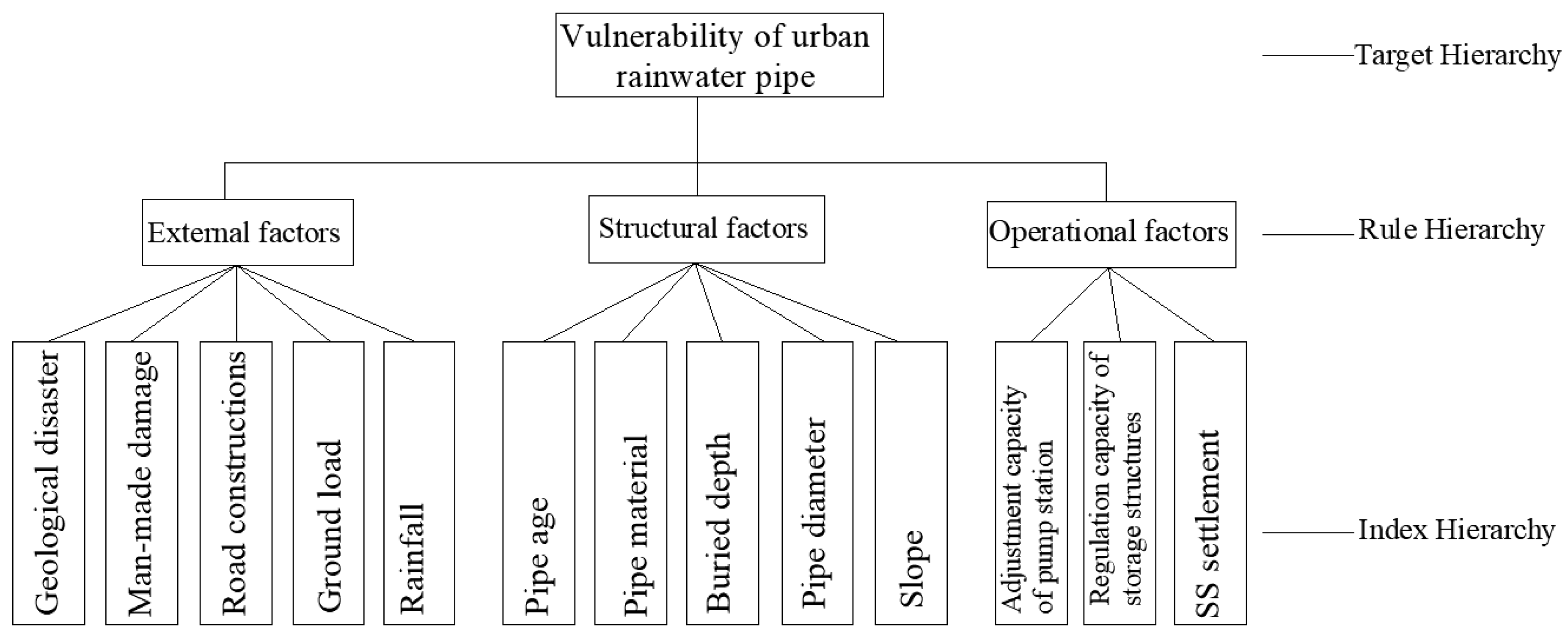
2. Evaluation Index

2.1. Index Selection

The urban rainwater pipe network is a complex system characterized by extensive pipelines, significant diameter variations, and substantial flow fluctuations. Taking into account its inherent rainwater discharge properties as well as the economic and social environment during urbanization, an index system is constructed that encompasses external factors, structural factors, and operational factors [48,49,50]. External factors include the impact of geological disasters, human-induced damage, road construction, ground load, and rainfall. The greater the degree of influence, the higher the vulnerability level. Structural factors are primarily assessed through aspects such as pipe age, pipe material, burial depth, pipe diameter, and slope. Operational factors mainly reflect the adjustment capacity of pump stations, the regulation capacity of storage structures, and SS (suspended solids) settlement. The specific index system is illustrated in Figure 1.

2.2. Data Selection Criteria

Referring to the “Standard for Design of Outdoor Wastewater Engineering” (GB50014-2021) and other relevant norms and standards, the index data level is divided into five distinct levels. The index value interval or score range for each grade is presented in

Table 1. Levels of the evaluation indicator system.

Secondary Index	Reference Range
	Excellent	Good	Medium	Poor	Flunk
	Very Safe Ⅰ	Safe Ⅱ	Relatively Safe Ⅲ	Dangerous Ⅳ	Very Dangerous Ⅴ
Geological disaster	No	Basically no	Seldom	More	Frequently
Man-made damage	No	Basically no	Seldom	More	Frequently
Road construction	Unexcavated	Excavation far away from the pipeline	Excavation near the pipeline	Excavation touches the pipeline	Large-scale excavation
Ground load	Tiny	Less	Average	Larger	Very large
Rainfall	<7 mm/h	7–17 mm/h	17–22 mm/h	22–33 mm/h	>33 mm/h
Pipe age	0–10 a	10–20 a	20–30 a	30–40 a	>40 a
Pipe material	HDPE	Cast iron pipe	Reinforced concrete pipe	Concrete pipe	Clay pipe
Buried depth	>2.5 m	2.0–2.5 m	1.0–1.5 m	0.7–1.0 m	<0.7 m
Pipe diameter	>DN1000	DN800–DN1000	DN500–DN800	DN300–DN500	<DN300
Slope	>10‰	4‰–10‰	2‰–4‰	1‰–2‰	<1‰
Capacity of pump station	>80 m3/s	40–80 m3/s	20–40 m3/s	10–20 m3/s	<10 m3/s
Regulation capacity of storage structures	>2000 m3	1000–2000 m3	500–1000 m3	100–500 m3	<100 m3
SS settlement	<20 mg/L	20–30 mg/L	30–40 mg/L	40–100 mg/L	>100 mg/L

.

3. The Combined Evaluation Method of Improved Fuzzy Borda

The traditional fuzzy Borda method and the improved fuzzy Borda method are unable to assign scores to individual drainage system samples. Therefore, an enhanced Borda method is proposed, taking into account both the best and worst solutions. This new combined method can utilize the evaluation results obtained from other methods. Four single evaluation methods are selected, including the entropy weight method, the gray correlation TOPSIS method, the efficiency coefficient method, and the fuzzy comprehensive evaluation method.

3.1. Single Evaluation Method

3.1.1. Entropy Weight Method

The entropy weight method is used to determine the importance of research objects. It is an objective evaluation method that eliminates subjective arbitrariness. This method assigns weights to indicators through calculations. Based on the computed results, a higher entropy indicates greater uncertainty and a smaller weight, while a lower entropy suggests less uncertainty and a larger weight. The entropy method is widely used due to its simple calculations and reliable results. The specific steps for evaluating the entropy weight method are as follows:

(1)

Establish the initial evaluation index matrix and dimensionless processing.

There are m evaluation objects, and each of them has n evaluation indexes. The initial evaluation index matrix X is established as:

$$X=\left[\begin{array}{cccc}{x}_{11}& x_{12}& \cdots & x_{1n}\\ x_{21}& x_{22}& \cdots & x_{2n}\\ ⋮& ⋮& \cdots & ⋮\\ x_{m1}& x_{m2}& \cdots & x_{mn}\end{array}\right]$$

(1)

the initial evaluation index matrix X is normalized to eliminate the influence of different dimensions of each index. The normalized matrix A is as follows:

$$A=\left[\begin{array}{cccc}{a}_{11}& a_{12}& \cdots & a_{1n}\\ a_{21}& a_{22}& \cdots & a_{2n}\\ ⋮& ⋮& \cdots & ⋮\\ a_{m1}& a_{m2}& \cdots & a_{mn}\end{array}\right]$$

(2)

for the positive index,

$$a_{ij}=\frac{x_{ij}-m_j}{M_j-m_j}$$

(3)

for the inverse index,

$$a_{ij}=\frac{M_j-x_{ij}}{M_j-m_j}$$

(4)

where a_ij is the normalized value of the initial evaluation index value; M_j is the maximum value of x_ij; and m_j is the minimum value of x_ij;

(2)

Calculate the information entropy of each index.

$$e_i=-\frac{1}{\ln n}{\displaystyle \sum _{i=1}^m{b}_{ij}\ln b_{ij}}$$

(5)

$$b_{ij}=a_{ij}/{\displaystyle \sum _{i=1}^m{a}_{ij}};$$

(6)

(3)

Calculate the weight of each indicator.

$${\epsilon }_j={\phi }_j/{\displaystyle \sum _{i=1}^n{\phi }_j}$$

(7)

where φ_j is the difference coefficient, φ_j = 1 − e_j and e is the base of the natural logarithm;

(4)

Calculate the score value of each sample.

$$Z_i=a_{ij}\times {\epsilon }_j$$

(8)

evaluation results can be obtained by ranking the scores from greatest to smallest.

3.1.2. Gray Correlation TOPSIS Method

The TOPSIS method is a ranking approach that approximates ideal solutions. By calculating the distance between each evaluation object and the positive and negative ideal solutions, the relative closeness degree is determined, which is then used to sort and evaluate the relative merits and demerits of each index [51].

However, this method’s discriminatory power is not very high. The gray correlation method can effectively address this issue. The calculation process for the gray correlation TOPSIS method is as follows:

(1)

Establish the initial evaluation index matrix and perform dimensionless processing.

The initial evaluation index matrix X (as shown in Formula (1)) is normalized using the sum of squares to eliminate the influence of different dimensions for each index. The resulting normalized matrix S is as follows:

$$S=\left[\begin{array}{cccc}{s}_{11}& s_{12}& \cdots & s_{1n}\\ s_{21}& s_{22}& \cdots & x_{2n}\\ ⋮& ⋮& \cdots & ⋮\\ s_{m1}& s_{m2}& \cdots & s_{mn}\end{array}\right]$$

(9)

$$s_{ij}=\frac{x_{ij}}{\sqrt{{\displaystyle \sum _{i=1}^m{x}_{ij}^2}}}$$

(10)

where s_ij is the normalized value of the initial evaluation index value;

(2)

Calculate the combination weight.

$${\omega }_i=\lambda {\eta }_i+(1-\lambda ){\epsilon }_i$$

(11)

where ω_i is the combination weight; η_i is the weight calculated by the analytic hierarchy process; ε_i is the weight calculated by the entropy weight method; λ is the decision coefficient, and 0 ≤ λ ≤ 1. The two methods are equally important, so the decision coefficient λ is taken as 0.5;

(3)

Calculate the weighted judgment matrix.

The weighted judgment matrix V is obtained by multiplying the normalized matrix with the combined weights of each index that have been previously determined.

$$V=\left[\begin{array}{cccc}{s}_{11}{\omega }_1& s_{12}{\omega }_2& \cdots & s_{1n}{\omega }_n\\ s_{21}{\omega }_1& s_{22}{\omega }_2& \cdots & x_{2n}{\omega }_n\\ ⋮& ⋮& \cdots & ⋮\\ s_{m1}{\omega }_1& s_{m2}{\omega }_2& \cdots & s_{mn}{\omega }_n\end{array}\right]=\left[\begin{array}{cccc}{v}_{11}& v_{12}& \cdots & v_{1n}\\ v_{21}& v_{22}& \cdots & v_{2n}\\ ⋮& ⋮& \cdots & ⋮\\ v_{m1}& v_{m2}& \cdots & v_{mn}\end{array}\right];$$

(12)

(4)

Determine the positive and negative ideal solutions.

For the “larger is better” type index, the positive and negative ideal solutions are, respectively, as follows:

$$\left\{\begin{array}{c}{v}_j^{+}=\max (v_{1j},v_{2j},\cdots ,v_{nj})\\ v_j^{-}=\min (v_{1j},v_{2j},\cdots ,v_{nj})\end{array}\right.$$

(13)

for the “smaller is better” type index, the positive and negative ideal solutions are, respectively, as follows:

$$\left\{\begin{array}{c}{v}_j^{+}=\min (v_{1j},v_{2j},\cdots ,v_{nj})\\ v_j^{-}=\max (v_{1j},v_{2j},\cdots ,v_{nj})\end{array}\right.;$$

(14)

(5)

Calculate the distance.

$$\left\{\begin{array}{c}{d}_i^{+}=\sqrt{{\displaystyle \sum _{j=1}^n{(v_j^{+}-v_{ij})}^2}}\\ d_i^{-}=\sqrt{{\displaystyle \sum _{j=1}^n{(v_j^{-}-v_{ij})}^2}}\end{array}\right.;$$

(15)

(6)

Calculate the gray correlation coefficient.

$$\left\{\begin{array}{c}{f}_{ij}^{+}=\frac{\underset{i=1}{\overset{m}{\min }}\underset{j=1}{\overset{n}{\min }}\left|v_j^{+}-v_{ij}\right|+\rho \underset{i=1}{\overset{m}{\max }}\underset{j=1}{\overset{n}{\max }}\left|v_j^{+}-v_{ij}\right|}{\left|v_j^{+}-v_{ij}\right|+\rho \underset{i=1}{\overset{m}{\max }}\underset{j=1}{\overset{n}{\max }}\left|v_j^{+}-v_{ij}\right|}\\ f_{ij}^{-}=\frac{\underset{i=1}{\overset{m}{\min }}\underset{j=1}{\overset{n}{\min }}\left|v_j^{-}-v_{ij}\right|+\rho \underset{i=1}{\overset{m}{\max }}\underset{j=1}{\overset{n}{\max }}\left|v_j^{-}-v_{ij}\right|}{\left|v_j^{-}-v_{ij}\right|+\rho \underset{i=1}{\overset{m}{\max }}\underset{j=1}{\overset{n}{\max }}\left|v_j^{-}-v_{ij}\right|}\end{array}\right.$$

(16)

where ρ is the discrimination coefficient, which is usually taken as 0.5;

(7)

Calculate the gray correlation degree.

$$\left\{\begin{array}{c}{r}_i^{+}=\frac{1}{n}{\displaystyle \sum _{j=1}^n{f}_{ij}^{+}}\\ r_i^{-}=\frac{1}{n}{\displaystyle \sum _{j=1}^n{f}_{ij}^{-}}\end{array}\right.;$$

(17)

(8)

Dimensionless processing formula.

$$\left\{\begin{array}{cc}\begin{array}{c}{D}_i^{+}=\frac{d_i^{+}}{\underset{i=1}{\overset{m}{\max }}\hspace{0.17em}{d}_i^{+}}\\ D_i^{-}=\frac{d_i^{-}}{\underset{i=1}{\overset{m}{\max }}\hspace{0.17em}{d}_i^{-}}\end{array}& \hspace{1em}\hspace{1em}\hspace{1em}\left\{\begin{array}{c}{R}_i^{+}=\frac{r_i^{+}}{\underset{i=1}{\overset{m}{\max }}\hspace{0.17em}{r}_i^{+}}\\ R_i^{-}=\frac{r_i^{-}}{\underset{i=1}{\overset{m}{\max }}\hspace{0.17em}{r}_i^{-}}\end{array}\right.;\end{array}\right.$$

(18)

(9)

Calculate the integrated distance.

$$\left\{\begin{array}{c}{E}_i^{+}={\alpha }_1{D}_i^{-}+{\alpha }_2{R}_i^{+}\\ E_i^{-}={\alpha }_1{D}_i^{+}+{\alpha }_2{R}_i^{-}\end{array}\right.$$

(19)

where ${\alpha }_1+{\alpha }_2=1$, ${\alpha }_1={\alpha }_2=0.5$;

(10)

Calculate the relative closeness.

$$C_i=\frac{E_i^{+}}{E_i^{+}+E_i^{-}}$$

(20)

the evaluation samples are ranked based on the closeness of the different samples. The higher the C_i value, the closer the evaluation samples are to the ideal solution.

3.1.3. Efficacy Coefficient Method

The efficiency coefficient method is an effective approach for comprehensive evaluation and multi-objective decision-making. It calculates the comprehensive evaluation value by combining the efficiency coefficients of multiple indicators with their weight coefficients. The specific calculation steps are as follows:

(1)

Calculate the efficiency coefficient for each index.

Due to the presence of both very large and very small index data, the calculations need to be performed separately.

The efficiency coefficients for very large index data are as follows:

$$g_{ij}=\left\{\begin{array}{c}\frac{c_{ij}-c_j^{″}}{c_j^{\prime }-c_j^{″}}\times 40+60,c_{ij}<c_j^{\prime }\\ 100,c_{ij}\ge c_j^{\prime }\end{array}\right.$$

(21)

the efficiency coefficients for very small index data are as follows:

$$g_{ij}=\left\{\begin{array}{c}\frac{\left|c_{ij}-c_j^{\prime }\right|}{c_j^{\prime }-c_j^{″}}\times 40+60,c_{ij}>c_j^{″}\\ 100,c_{ij}\le c_j^{″}\end{array}\right.$$

(22)

where $c_j^{\prime }$ and $c_j^{″}$ are the upper and lower limits of the allowable value of index j;

(2)

The weight value η_i of each index is determined by the analytic hierarchy process or combination weight determination method;

(3)

The evaluation scores $B_i={{\displaystyle \sum }}_{j=1}^k{g}_{ij}\times {\eta }_i$ of each sample are calculated and sorted according to the score value from large to small.

3.1.4. Fuzzy Comprehensive Evaluation Method

The fuzzy comprehensive evaluation method is a combined evaluation approach that integrates both qualitative and quantitative analysis. This method divides the membership degree levels of the evaluated items, performing comprehensive evaluations using multiple indices from different perspectives based on fuzzy sets. The fuzziness of evaluation criteria and the uncertainty of influencing factors arising from different hierarchical relationships among evaluation objects are considered. At the same time, subjective input can also be taken into account, making the final calculation result more objective and realistic. The calculation steps are as follows:

(1)

Determine the weight of each index and quantify the evaluated object on each index, Ui. This involves determining the membership degree of the evaluated object in each level subset ($\mathsf{\Lambda }/U_i$) from a single factor, and then obtaining the fuzzy relationship matrix.

$$\Lambda =\left[\begin{array}{c}\Lambda /U_1\\ \Lambda /U_2\\ ⋮\\ \Lambda /U_m\end{array}\right]={\left[\begin{array}{cccc}{\mu }_{11}& {\mu }_{12}& \cdots & {\mu }_{1k}\\ {\mu }_{21}& {\mu }_{22}& \cdots & {\mu }_{2k}\\ ⋮& ⋮& & ⋮\\ {\mu }_{m1}& {\mu }_{m2}& \cdots & {\mu }_{mk}\end{array}\right]}_{m\times k}$$

(23)

${\mu }_{ij}$ is the element of row i and column j in the matrix $\mathsf{\Lambda }$. ${\mu }_{ij}$ represents the membership degree of the evaluation index rated as grade $V_i\left(j=1,2,\cdots ,k\right)$ from the perspective of facto $U_i$. The rating proportion is used to determine the membership function of each index in the model. In other words, ${\mu }_{ij}={\varphi }_j/\varphi$ in the above expression, where ϕ is the number of participating experts in the evaluation, ${\varphi }_j$ is the number of experts assigning the first j evaluation scale Vj for the ith evaluation index, m is the number of evaluation indices, and k is the judging level (k = 5);

(2)

The comprehensive evaluation set of a certain level index is $Q=\Omega \mathsf{\Lambda }$.

• where $\Omega$ is the weight vector of each factor and $\mathsf{\Lambda }$ is the fuzzy matrix.

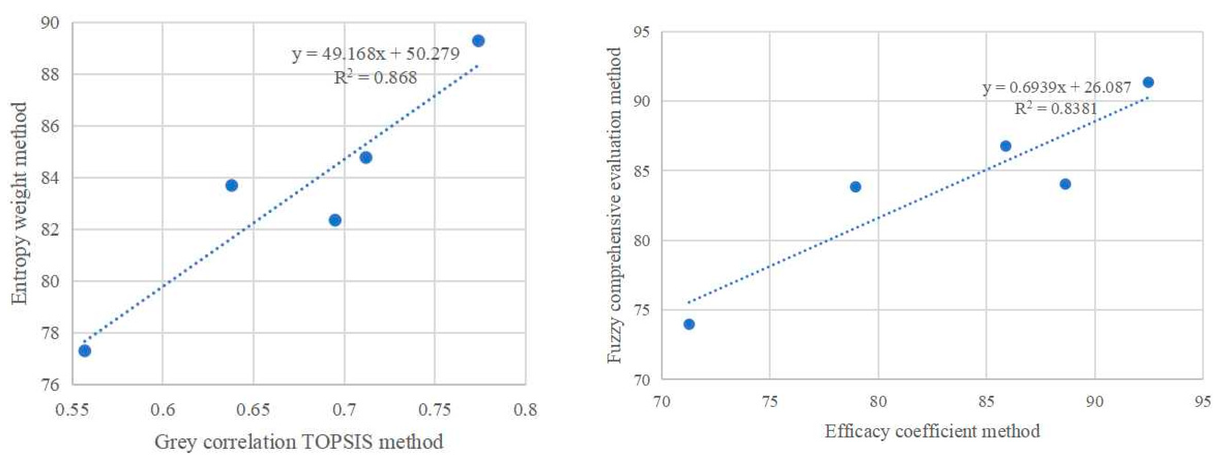
3.2. Ante-Test of Combined Evaluation Methods

The results of the selected single evaluation methods need to be checked for consistency to ensure the compatibility of each individual evaluation method. This allows the single methods to be verified against each other, and the combined evaluation results can be obtained with high credibility. Since there are four single evaluation methods for combinations, the Kendall method is used for the preliminary test. For n evaluated objects and one single evaluation method, the null hypothesis states that the evaluation results of one single evaluation method are not consistent. Conversely, the alternative hypothesis states that the evaluation results of the single evaluation method are consistent. The critical values of the test statistic and Kendall’s consistency coefficient are as follows:

$$\left\{\begin{array}{c}\Pi ={\displaystyle \sum _{i=1}^n{Y}_i^2-1/n\times {({\displaystyle \sum _{i=1}^n{Y}_i})}^2,{\Pi }_{\alpha },l<7}\\ {\chi }^2=l\times (n-1)\times W,X_{\alpha }^2(n-1),l>7\end{array}\right.$$

(24)

where $\Pi$ and ${\chi }^2$ are the test statistics for the different numbers of evaluation methods; the average ranking of any sample,

$$X_i={\displaystyle \sum _{z=1}^l{x}_{iz}}$$

(25)

where $x_{iz}$ represents the ranking of the ith stormwater pipe network system using the zth method; ${\Pi }_{\alpha }$ and $X_{\alpha }^2\left(n-1\right)$ are the critical values of the Kendall consistency coefficient for different evaluation methods under a known significance level, which can be obtained by referring to the Kendall consistency coefficient critical value table. W is Kendall’s coefficient of concordance.

$$W=(12{\displaystyle \sum _{i=1}^n{X}_i^2})/(n^2\times l\times (l^2-1))-3(l+1)/(l-1)$$

(26)

The null hypothesis is rejected as $\Pi >{\Pi }_{\alpha }$ or ${\chi }^2>X_{\alpha }^2\left(n-1\right)$. The evaluation results can be considered consistent, and the combined evaluation can be carried out.

3.3. Back Testing of Combined Evaluation Methods

The Spearman rank correlation coefficient method is typically used to test the validity of the combined evaluation results. ${\zeta }_j$ is the Spearman rank correlation coefficient for each single evaluation method or combined method.

The null hypothesis proposes that the combined evaluation method is unrelated to each single evaluation method. The alternative hypothesis is that the combined evaluation method has a strong correlation with each single evaluation method. The test statistic is calculated as follows:

$$\left\{\begin{array}{c}\rho =\frac{1}{l}{\displaystyle \sum _{j=1}^l{\zeta }_j},n<10\\ t_{\alpha }=(\frac{1}{l}{\displaystyle \sum _{j=1}^l{\zeta }_j})\sqrt{(n-2)/(1-{(\frac{1}{l}{\displaystyle \sum _{j=1}^l{\zeta }_j})}^2)},n\ge 10\end{array}\right.$$

(27)

where t_α is the T-distribution with n-2 degrees of freedom and n is the number of samples.

The null hypothesis is rejected when the statistical value is greater than the critical value, indicating a strong connection between the combined evaluation method and the single evaluation method. In this case, the backtesting of the combined evaluation method is considered successful.

3.4. Improved Fuzzy Borda Combination Evaluation Method

The fuzzy Borda combination evaluation method can synthesize different results from various evaluation methods. It takes into account both the difference in rankings under different methods and the scores of various items under the corresponding evaluation methods. This approach allows for better utilization of single evaluation information, resulting in higher rationality and superiority [52,53].

The specific steps of the improved fuzzy Borda combination evaluation method are as follows:

(1)

Use each single evaluation method to evaluate objects, and perform a preliminary test of the combination method using the Kendall method. If the test fails, recombine the single evaluation methods and test again. If the test is successful, proceed to the next step;

(2)

Calculate the membership degree $u_{ij}$ of “excellent” for the ith project using the jth evaluation method:

$$\begin{gathered} u_{ij}=\frac{y_{ij}-\underset{i}{\min }\left\{y_{ij}\right\}}{\underset{i}{\max }\left\{y_{ij}\right\}-\underset{i}{\min }\left\{y_{ij}\right\}}\times 0.9+0.1 \\ (i=1,2,\dots ,n;j=1,2,\cdots ,l); \end{gathered}$$

(28)

(3)

Calculate the No. h fuzzy frequency $w_{ih}$ of the No. i sample:

$$\mathrm{Fuzzy} \mathrm{frequency}: P_{ih}={{\displaystyle \sum }}_{i=1}^n{\delta }_{ij}^h{u}_{ij}\left(i=1,2,\cdots ,n;h=1,2,\cdots ,n\right)$$

(29)

where ${\delta }_{ij}^h=1,\mathrm{No}.i s\mathrm{ample} \mathrm{ranks} h \mathrm{in} \mathrm{the} \mathrm{No}.j \mathrm{evaluation} \mathrm{method}$

$${\delta }_{ij}^h=0,else$$

if the two samples rank the same, take 1/2, and so on.

$$\mathrm{Fuzzy} \mathrm{frequency}: w_{ih}=\frac{P_{ih}}{F_i}\left(i=1,2,\dots ,n\right)$$

(30)

where $F_i={{\displaystyle \sum }}_{h=1}^n{P}_{ih}\left(i=1,2,\dots ,n\right)$;

(4)

Calculate the fuzzy Borda number Bi of each process:

$$\mathrm{Convert} \mathrm{ranking} \mathrm{to} \mathrm{score}: Q_{ih}=\frac{\left(n-h\right)\left(n-h+1\right)}{2}$$

(31)

$$\mathrm{fuzzy} \mathrm{Borda} \mathrm{number}: B_i={{\displaystyle \sum }}_{h=1}^n{w}_{ih}{Q}_{ih}\left(i=1,2,\dots ,n\right)$$

(32)

sort from top to bottom according to fuzzy Borda number;

(5)

Back testing: if passed, go to the next step; otherwise, go to step (2);

(6)

Establish the comparison of rainwater system samples: $q^{\prime }=\left\{\left.\left\{q_{i1},q_{i2},\cdots ,q_{ik}\right\}\right|F_{qi}=\max \left\{F_i\right\}\right\}$ and $q^{\prime }=\left\{\left.\left\{q_{i1},q_{i2},\cdots ,q_{ik}\right\}\right|F_{qi}=\max \left\{F_i\right\}\right\}$. The combination evaluation score is $B^{\prime }$ and $B^{″}$. The final combination score can be obtained according to various gradient differences in fuzzy Borda numbers between the samples $q^{\prime }$ and $q^{″}$.

$B^{\prime }$ and $B^{″}$ are determined as follows:

Five grade standards are set for index j,

$$o_j=\left\{o_j\left(1\right),o_j\left(2\right),o_j\left(3\right),o_j\left(4\right),o_j\left(5\right)\right\}$$

(33)

the correlation degree between $q^{\prime }$ and $q^{″}$ at all levels is calculated.

When the evaluation index is “very poor”, the value of $u_{j1}^l$ can be:

$$\left.-1\right|q_j\in \left[o_j(0),o_j(1)\right];\left.1+2\frac{q_j-o_j(1)}{o_j(2)-x}\right|q_j\in \left[o_j(1),o_j(2)\right];\left.-1\right|q_j\in \left[o_j(2),o_j(5)\right]$$

(34)

when the evaluation index is “poor”, the value of $u_{j2}^l$ can be:

$$\left.1+2\frac{q_j-o_j(1)}{o_j(0)-x}\right|q_j\in \left[o_j(0),o_j(1)\right];\left.1\right|q_j\in \left[o_j(1),o_j(2)\right];$$

$$\left.1+2\frac{q_j-o_j(2)}{o_j(3)-x}\right|q_j\in \left[o_j(2),o_j(3)\right];-\left.1\right|q_j\in \left[o_j(3),o_j(5)\right]$$

(35)

when the evaluation index is “medium”, the value of $u_{j3}^l$ can be:

$$\left.-1\right|q_j\in \left[o_j(0),o_j(1)\right];\left.1+2\frac{q_j-o_j(2)}{o_j(1)-q_j}\right|q_j\in \left[o_j(1),o_j(2)\right];$$

$$\left.1\right|q_j\in \left[o_j(2),o_j(3)\right];\left.1+2\frac{q_j-o_j(3)}{o_j(4)-q_j}\right|q_j\in \left[o_j(3),o_j(4)\right];\left.-1\right|q_j\in \left[o_j(4),o_j(5)\right]$$

(36)

when the evaluation index is “good”, the value of $u_{j4}^l$ can be:

$$\left.-1\right|q_j\in \left[o_j(0),o_j(2)\right];\left.1+2\frac{q_j-o_j(3)}{o_j(2)-q_j}\right|q_j\in \left[o_j(2),o_j(3)\right];$$

$$\left.1\right|q_j\in \left[o_j(3),o_j(4)\right];\left.1+2\frac{q_j-o_j(4)}{o_j(5)-q_j}\right|q_j\in \left[o_j(4),o_j(5)\right]$$

(37)

when the evaluation index is “excellent”, the value of $u_{j5}^l$ can be:

$$\left.-1\right|q_j\in \left[o_j(0),o_j(3)\right];\left.1+2\frac{q_j-o_j(4)}{o_j(2)-o_j(4)}\right|q_j\in \left[o_j(3),o_j(4)\right];\left.1\right|q_j\in \left[o_j(4),o_j(5)\right]$$

(38)

where $o_j=\left\{o_j\left(1\right),o_j\left(2\right),o_j\left(3\right),o_j\left(4\right),o_j\left(5\right)\right\}$ is the boundary value corresponding to the grade division interval. There is a relationship of $o_j\left(0\right)<o_j\left(1\right)<\cdots <o_j\left(5\right)$ with the benefit type index. There is a relationship of $o_j\left(0\right)>o_j\left(1\right)>\cdots >o_j\left(5\right)$ with the cost type index. $q_j$ is the index data to be evaluated. The proportion belonging to each level $\lambda \left(o_j\right)$ is obtained by normalizing the correlation degree between each index and different levels. The score gradient of five levels is set as ${[{\upsilon }_j]}_{1\times 5}=\left[0,40,60,80,100\right]$. The score of samples $q^{\prime }$ and $q^{″}$ is calculated as follows by combining the index weight $y_j$.

$$B^{\prime }={\displaystyle \sum _{j=1}^5{\upsilon }_j\times {\lambda }_q^{\prime }(o_j)\times y_j}, B^{″}={\displaystyle \sum _{j=1}^5{\upsilon }_j\times {\lambda }_q^{″}(o_j)\times y_j}.$$

(39)

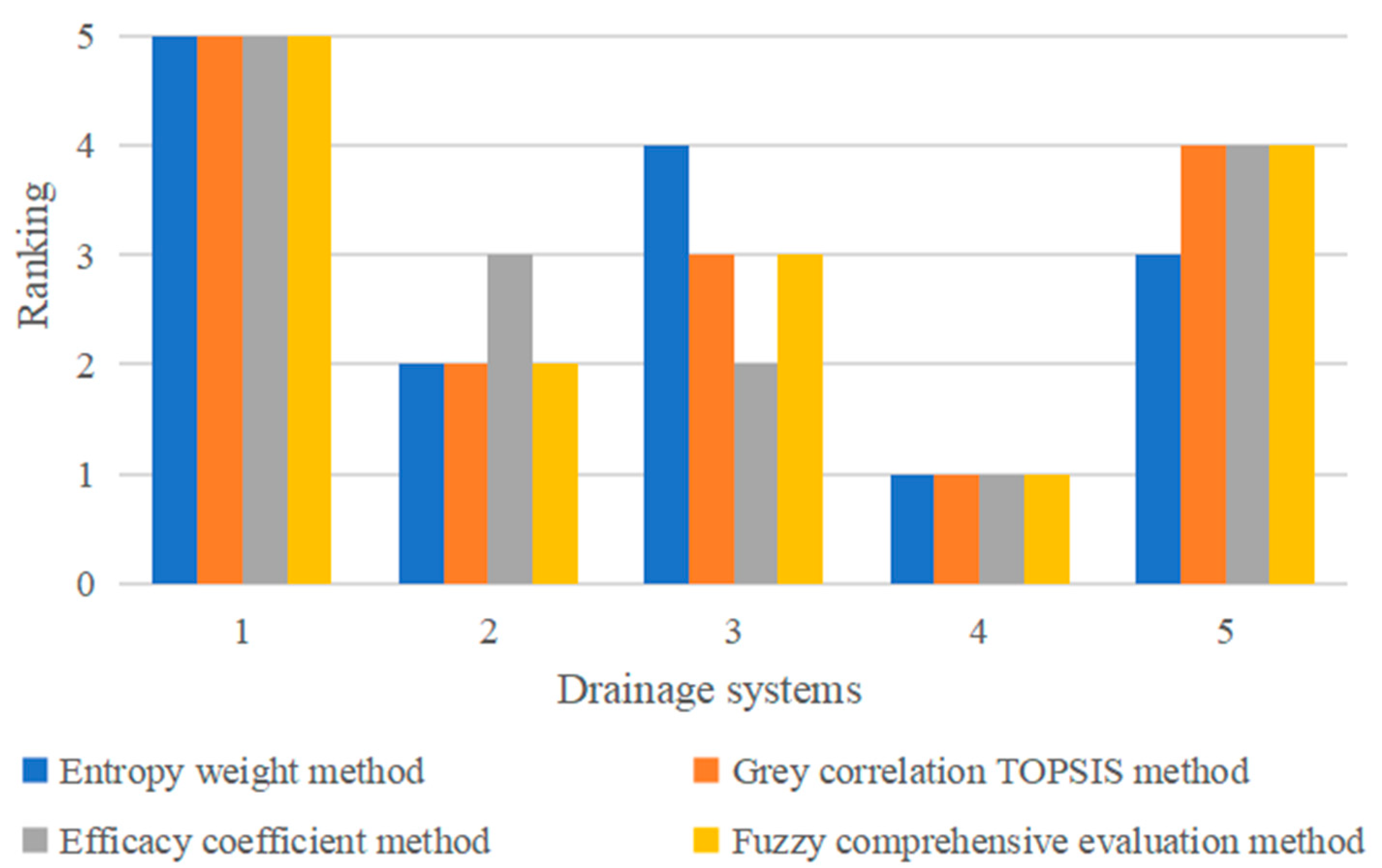
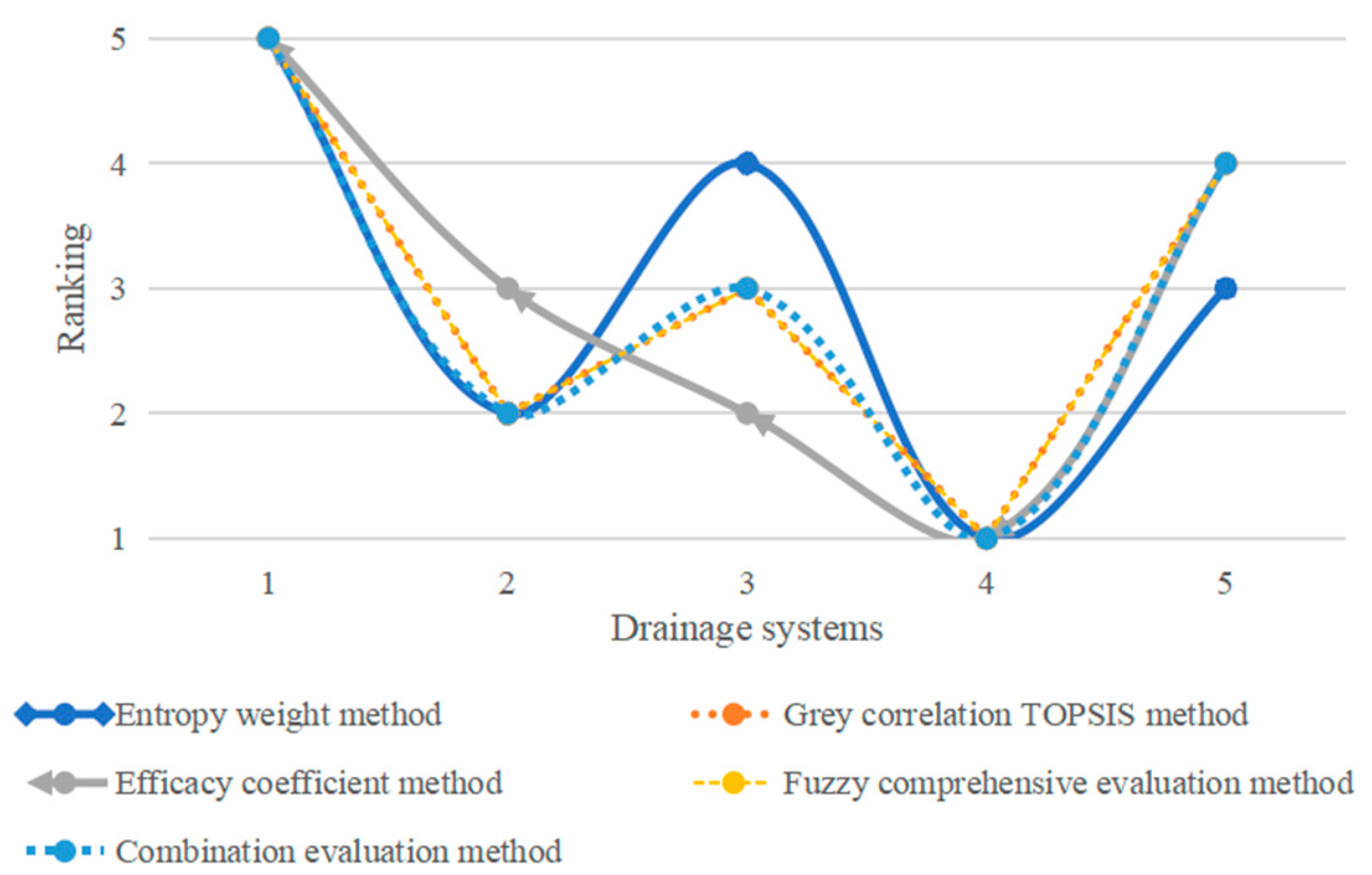
4. Case Study

Case Background

The capital city of Central China is naturally divided into three districts by the Yangtze River and the Han River. The city features numerous lakes and rivers, resulting in over 20 relatively independent drainage systems within the urban area. In this study, five drainage systems are selected as sample cases for analysis, and the relevant evaluation index data is presented in

Table 2. Index data for drainage systems.

Evaluation Index	Drainage System 1	Drainage System 2	Drainage System 3	Drainage System 4	Drainage System 5
Geological disaster	Seldom	Basically no	Seldom	Basically no	Basically no
Man-made damage	More	Seldom	Seldom	Basically no	Basically no
Road construction	Excavation near the pipeline	Excavation far away from the pipeline	Excavation touch pipeline	Excavation far away from the pipeline	Excavation far away from the pipeline
Ground load	Average	Less	Larger	Less	Larger
Rainfall	7–17 mm/h	17–22 mm/h	17–22 mm/h	17–22 mm/h	7–17 mm/h
Pipe age	30–40 a	10–20 a	20–30 a	10–20 a	20–30 a
Pipe material	Concrete pipe	Reinforced concrete pipe	Concrete pipe	Reinforced concrete pipe	Concrete pipe
Buried depth	1.5–2.0 m	2.0–2.5 m	2.0–2.5 m	>2.5 m	>2.5 m
Pipe diameter	DN300–DN500	>DN1000	DN500–DN800	>DN1000	DN500–DN800
Slope	2‰–4‰	4‰–10‰	2‰–4‰	4‰–10‰	2‰–4‰
Capacity of the pump station	10–20 m3/s	40–80 m3/s	20–40 m3/s	40–80 m3/s	20–40 m3/s
Regulation of the capacity of storage structures	500–1000 m3	1000–2000 m3	1000–2000 m3	500–1000 m3	500–1000 m3
SS settlement	>100 mg/L	20–30 mg/L	30–40 mg/L	30–40 mg/L	30–40 mg/L

.

The aforementioned five drainage systems were assessed using the single evaluation method, and the results are displayed in

Table 3. Evaluation results by four single evaluation methods.

No.	Entropy Weight Method		Gray Correlation TOPSIS Method		Efficacy Coefficient Method		Fuzzy Comprehensive Evaluation Method
	Evaluation Value	Ranking	Evaluation Value	Ranking	Evaluation Value	Ranking	Evaluation Value	Ranking
1	77.30	5	0.557	5	71.28	5	73.97	5
2	84.77	2	0.712	2	85.89	3	86.77	2
3	82.35	4	0.695	3	88.64	2	84.04	3
4	89.28	1	0.774	1	92.47	1	91.35	1
5	83.69	3	0.638	4	78.96	4	83.84	4

.

The Kendall method was used for the preliminary test. The null hypothesis H0 was proposed, suggesting that the evaluation results obtained by the four single evaluation methods were inconsistent. The significance level was set at 0.01, and the test statistic was calculated to be 124. The critical value of the Kendall consistency coefficient was 109.3, as found in the table. Thus, the null hypothesis was rejected. The Kendall-W concordance coefficient was used to further test the significance. When the concordance coefficient W is closer to 1, the consistency between the data is stronger. The calculated concordance coefficient, as shown in

Table 4. Kendall correlation coefficient of a single evaluation model.

Kendall Correlation Coefficient	Entropy Weight Method	Gray Correlation TOPSIS Method	Efficacy Coefficient Method	Fuzzy Comprehensive Evaluation Method
Entropy weight method	1
Gray correlation TOPSIS method	0.916	1
Efficacy coefficient method	0.783	0.886	1
Fuzzy comprehensive evaluation method	0.916	1	0.908	1

, indicates high consistency among the four single evaluations. They passed the preliminary consistency test.

The scatterplot of the four single evaluation methods is displayed in Figure 2, and the histogram can be seen in Figure 3. From Figure 2 and Figure 3, the evaluation results of each method are consistent and meet the necessary conditions for a combined evaluation. The correlation coefficient of each single evaluation method was calculated, with the minimum value being 0.9155. The results obtained by any two evaluation methods exhibited a high correlation. Based on these results, a combination analysis was performed. The combined scores of each sample were obtained using the improved fuzzy Borda combination evaluation method, as shown in

Table 5. Sample ranking by combination evaluation results.

No.	Combination Evaluation Results
	Combined Score	Ranking
1	74.06	5
2	86.45	2
3	79.25	3
4	90.37	1
5	75.88	4

.

After obtaining the combined evaluation results, the Spearman rank correlation coefficient method should be used for the backtesting. Given that there are five evaluated samples, the calculated test statistic is 0.975. Under the significance level of 0.05, the critical value of the consistency coefficient is 0.9, as found in the table. The null hypothesis is rejected, and the combined evaluation results are considered consistent. They passed the backtesting. The ranking of samples in the combined evaluation method and each single evaluation method is shown in Figure 4.

As can be seen from Figure 4, the results exhibit high consistency. The compatibility of the five evaluation methods was calculated, as displayed in

Table 6. Compatibility between evaluation methods.

Spearman Rank Correlation Coefficient	Entropy Weight Method	Gray Correlation TOPSIS Method	Efficacy Coefficient Method	Fuzzy Comprehensive Evaluation Method	Combination Evaluation
Entropy weight method	1
Gray correlation TOPSIS method	0.941	1
Efficacy coefficient method	0.884	0.902	1
Fuzzy comprehensive evaluation method	0.941	1	0.923	1
Combination evaluation	0.941	1	0.923	1	1
Compatibility	0.906	0.9755	0.949	1	1

.

Table 6 shows that the compatibility of the combined evaluation method is greater than or equal to that of the other methods, indicating high credibility. The combined evaluation results in Table 6 reveal that the score of water system 4 is the highest, which is consistent with the other single evaluation methods. This confirms the principle that the minority is subordinate to the majority in the fuzzy Borda method.

5. Conclusions

Various methods can be used to evaluate the vulnerability of rainwater pipe networks. Although there are some differences in the evaluation results of different methods, the overall evaluation results are similar. The improved fuzzy Borda combination evaluation method can comprehensively analyze deterministic and uncertain elements in the system and improve the reliability of the evaluation results. In this case, the compatibility of the combined method is 0.96, indicating high credibility. By calculating the fuzzy Borda numbers, positive and negative ideal drainage system samples, and correlation degrees at all levels, the comprehensive evaluation value of each drainage system sample can be obtained. Referring to the optimal sample, drainage system parameters can be reasonably set in the future. Although the proposed model has high credibility, its calculation is more complex compared to single evaluation methods. Moreover, the dynamic development of system indicators is not considered in the evaluation process, which requires further research.

References

- Awolala, D.O.; Ajibefun, I.A.; Ogunjobi, K.; Miao, R. Integrated assessment of human vulnerability to extreme climate hazards: Emerging outcomes for adaptation finance allocation in Southwest Nigeria. Clim. Dev. 2021, 14, 166–183. [Google Scholar] [CrossRef]
- Wang, L.; Huang, S.; Huang, Q.; Leng, G.; Han, Z.; Zhao, J.; Guo, Y. Vegetation vulnerability and resistance to hydrometeorological stresses in water-and energylimited watersheds based on a Bayesian framework. Catena 2021, 196, 104879. [Google Scholar] [CrossRef]
- Karmaoui, A.; Balica, S. A new flood vulnerability index adapted for the preSaharan region. Int. J. River Basin Manag. 2021, 19, 93–107. [Google Scholar] [CrossRef]
- Shen, Y.; Morsy, M.; Huxley, C.; Tahvildari, N.; Goodall, J. Flood risk assessment and increased resilience for coastal urban watersheds under the combined impact of storm tide and heavy rainfall. J. Hydrol. 2019, 579, 124159. [Google Scholar] [CrossRef]
- Kim, D.Y.; Park, S.H.; Song, C.M. Evaluation of water social service and comprehensive water management linked with integrated river evaluation. Water 2021, 13, 706. [Google Scholar] [CrossRef]
- Soonthornrangsan, J.T.; Lowry, C.S. Vulnerability of water resources under a changing climate and human activity in the lower Great Lakes region. Hydrol. Process. 2021, 35, e14440. [Google Scholar] [CrossRef]
- Zhang, M.; Xu, M.; Wang, Z.; Lai, C. Assessment of the vulnerability of road networks to urban waterlogging based on a coupled hydrodynamic model. J. Hydrol. 2021, 603, 127105. [Google Scholar] [CrossRef]
- Mafi-Gholami, D.; Pirasteh, S.; Ellison, J.C.; Jaafari, A. Fuzzy-based vulnerability assessment of coupled social-ecological systems to multiple environmental hazards and climate change. J. Environ. Manag. 2021, 299, 113573. [Google Scholar] [CrossRef]
- Khosravi, K.; Shahabi, H.; Pham, B.T.; Adamowski, J.; Shirzadi, A.; Pradhan, B.; Prakash, I. A comparative assessment of flood susceptibility modeling using multi-criteria decision-making analysis and machine learning methods. J. Hydrol. 2019, 573, 311–323. [Google Scholar] [CrossRef]
- Xiao, Y.; Tang, X.; Li, Y.; Huang, H.; An, B.W. Social vulnerability assessment of landslide disaster based on improved TOPSIS method: Case study of eleven small towns in China. Ecol. Indic. 2022, 143, 109316. [Google Scholar] [CrossRef]
- Roy, S.; Debnath, P.; Mitra, S. Impact of Climate Disasters on Railway Infrastructure: Case Study of Northeast India. Acadlore Trans. Geosci. 2023, 2, 33–45. [Google Scholar] [CrossRef]
- Lachaut, T.; Yoon, J.; Klassert, C.; Tilmant, A. Aggregation in bottom-up vulnerability assessments and equity implications: The case of Jordanian households’ water supply. Adv. Water Resour. 2022, 169, 104311. [Google Scholar] [CrossRef]
- Zhang, X.; Zhao, X.; Li, R.; Mao, G.; Tillotson, M.R.; Liao, X.; Yi, Y. Evaluating the vulnerability of physical and virtual water resource networks in China’s megacities. Resour. Conserv. Recycl. 2020, 161, 104972. [Google Scholar] [CrossRef]
- Ruidas, D.; Pal, S.C.; Saha, A.; Chowdhuri, I.; Shit, M. Hydrogeochemical characterization based water resources vulnerability assessment in India’s first Ramsar site of Chilka lake. Mar. Pollut. Bull. 2022, 184, 114107. [Google Scholar] [CrossRef]
- Gui, Z.; Chen, X.; He, Y. Spatiotemporal analysis of water resources system vulnerability in the Lancang River Basin, China. J. Hydrol. 2021, 601, 126614. [Google Scholar] [CrossRef]
- Obradovic, V.; Vulevic, A. Water Resources Protection and Water Management Framework in Western Balkan Countries in Drina River Basin. Acadlore Trans. Geosci. 2023, 2, 24–32. [Google Scholar] [CrossRef]
- Dhaoui, O.; Antunes, I.M.H.R.; Agoubi, B.; Kharroubi, A. Integration of water contamination indicators and vulnerability indices on groundwater management in Menzel Habib area, south-eastern Tunisia. Environ. Res. 2022, 205, 112491. [Google Scholar] [CrossRef]
- Kumar, P.; Sharma, R.; Bhaumik, S. MCDA techniques used in optimization of weights and ratings of DRASTIC model for groundwater vulnerability assessment. Data Sci. Manag. 2022, 5, 28–41. [Google Scholar] [CrossRef]
- Zanotti, C.; Rotiroti, M.; Caschetto, M.; Redaelli, A.; Bozza, S.; Biasibetti, M.; Bonomi, T. A cost-effective method for assessing groundwater well vulnerability to anthropogenic and natural pollution in the framework of water safety plans. J. Hydrol. 2022, 613, 128473. [Google Scholar] [CrossRef]
- Sun, M.; Kato, T. Spatial-temporal analysis of urban water resource vulnerability in China. Ecol. Indic. 2021, 133, 108436. [Google Scholar] [CrossRef]
- Islam, A.R.M.T.; Pal, S.C.; Chakrabortty, R.; Idris, A.M.; Salam, R.; Islam, M.S.; Ismail, Z.B. A coupled novel framework for assessing vulnerability of water resources using hydrochemical analysis and data-driven models. J. Clean. Prod. 2022, 336, 130407. [Google Scholar] [CrossRef]
- Bibi, T.S.; Kara, K.G.; Bedada, H.J.; Bededa, R.D. Application of PCSWMM for assessing the impacts of urbanization and climate changes on the efficiency of stormwater drainage systems in managing urban flooding in Robe town, Ethiopia. J. Hydrol. Reg. Stud. 2023, 45, 101291. [Google Scholar] [CrossRef]
- Rahman, M.; Haque, M.M.; Tareq, S.M. Appraisal of groundwater vulnerability in south-central part of Bangladesh using DRASTIC model: An approach towards groundwater protection and health safety. Environ. Chall. 2021, 5, 100391. [Google Scholar] [CrossRef]
- Thapa, R.; Gupta, S.; Guin, S.; Kaur, H. Sensitivity analysis and mapping the potential groundwater vulnerability zones in Birbhum district, India: A comparative approach between vulnerability models. Water Sci. 2018, 32, 44–66. [Google Scholar] [CrossRef]
- Rajput, H.; Goyal, R.; Brighu, U. Modification and optimization of DRASTIC model for groundwater vulnerability and contamination risk assessment for Bhiwadi region of Rajasthan, India. Environ. Earth Sci. 2020, 79, 136. [Google Scholar] [CrossRef]
- Voutchkova, D.D.; Schullehner, J.; Rasmussen, P.; Hansen, B. A high-resolution nitrate vulnerability assessment of sandy aquifers (DRASTIC-N). J. Environ. Manag. 2021, 277, 111330. [Google Scholar] [CrossRef] [PubMed]
- Liang, J.; Li, Z.; Yang, Q.; Lei, X.; Kang, A.; Li, S. Specific vulnerability assessment of nitrate in shallow groundwater with an improved DRSTIC-LE model. Ecotoxicol. Environ. Saf. 2019, 174, 649–657. [Google Scholar] [CrossRef] [PubMed]
- Neshat, A.; Pradhan, B.; Dadras, M. Groundwater vulnerability assessment using an improved DRASTIC method in GIS. Resour. Conserv. Recycl. 2014, 86, 74–86. [Google Scholar] [CrossRef]
- Birawida, A.B.; Ibrahim, E.; Mallongi, A.; Al Rasyidi, A.A.; Thamrin, Y.; Gunawan, N.A. Clean water supply vulnerability model for improving the quality of public health (environmental health perspective): A case in Spermonde islands, Makassar Indonesia. Gac. Sanit. 2021, 35, S601–S603. [Google Scholar] [CrossRef]
- Abdullah, T.O.; Ali, S.S.; Al-Ansari, N.A.; Knutsson, S. Assessment of groundwater vulnerability to pollution using two different vulnerability models in Halabja-Saidsadiq Basin, Iraq. Groundw. Sustain. Dev. 2020, 10, 100276. [Google Scholar] [CrossRef]
- Dong, Y.; Zhou, W.; Wang, X.; Lu, Y.; Zhao, P.; Li, X. A new assessment method for the vulnerability of confined water: WF &PNN method. J. Hydrol. 2020, 590, 125217. [Google Scholar] [CrossRef]
- Barzegar, R.; Razzagh, S.; Quilty, J.; Adamowski, J.; Pour, H.K.; Booij, M.J. Improving GALDIT-based groundwater vulnerability predictive mapping using coupled resampling algorithms and machine learning models. J. Hydrol. 2021, 598, 126370. [Google Scholar] [CrossRef]
- Khashei-Siuki, A.; Sharifan, H. Comparison of AHP and FAHP methods in determining suitable areas for drinking water harvesting in Birjand aquifer. Iran. Groundw. Sustain. Dev. 2020, 10, 100328. [Google Scholar] [CrossRef]
- Ghosh, S.; Das, A. Urban expansion induced vulnerability assessment of East Kolkata Wetland using Fuzzy MCDM method. Remote Sens. Appl. Soc. Environ. 2019, 13, 191–203. [Google Scholar] [CrossRef]
- Sahana, M.; Rehman, S.; Sajjad, H.; Hong, H. Exploring effectiveness of frequency ratio and support vector machine models in storm surge flood susceptibility assessment: A study of Sundarban Biosphere Reserve, India. Catena 2020, 189, 104450. [Google Scholar] [CrossRef]
- Ameri, A.A.; Pourghasemi, H.R.; Cerda, A. Erodibility prioritization of sub-watersheds using morphometric parameters analysis and its mapping: A comparison among TOPSIS, VIKOR, SAW, and CF multi-criteria decision making models. Sci. Total Environ. 2018, 613, 1385–1400. [Google Scholar] [CrossRef]
- Sarkar, P.; Kumar, P.; Vishwakarma, D.K.; Ashok, A.; Elbeltagi, A.; Gupta, S.; Kuriqi, A. Watershed prioritization using morphometric analysis by MCDM approaches. Ecol. Inform. 2022, 70, 101763. [Google Scholar] [CrossRef]
- Yao, L.; Shuai, Y.; Chen, X. Regional water system vulnerability evaluation: A bi-level DEA with multi-followers approach. J. Hydrol. 2020, 589, 125160. [Google Scholar] [CrossRef]
- Yang, Y.; Guo, H.; Wang, D.; Ke, X.; Li, S.; Huang, S. Flood vulnerability and resilience assessment in China based on super-efficiency DEA and SBM-DEA methods. J. Hydrol. 2021, 600, 126470. [Google Scholar] [CrossRef]
- Li, J.; He, W.S.; Tai, S.Y.; Miao, K.Y. Evaluation of water resources carrying capacity in Gansu Province based on combined weight and grey correlation TOPSIS method. Sci. Technol. Eng. 2021, 21, 7327–7333. [Google Scholar] [CrossRef]
- Ali, M.; Prasad, R.; Xiang, Y.; Yaseen, Z.M. Complete ensemble empirical mode decomposition hybridized with random forest and kernel ridge regression model for monthly rainfall forecasts. J. Hydrol. 2020, 584, 124647. [Google Scholar] [CrossRef]
- Gad, M.; El-Safa, A.; Magda, M.; Farouk, M.; Hussein, H.; Alnemari, A.M.; Saleh, A.H. Integration of water quality indices and multivariate modeling for assessing surface water quality in Qaroun Lake, Egypt. Water 2021, 13, 2258. [Google Scholar] [CrossRef]
- Hu, X.; Ma, C.; Huang, P.; Guo, X. Ecological vulnerability assessment based on AHP-PSR method and analysis of its single parameter sensitivity and spatial autocorrelation for ecological protection–A case of Weifang City, China. Ecol. Indic. 2021, 125, 107464. [Google Scholar] [CrossRef]
- Dodangeh, E.; Choubin, B.; Eigdir, A.N.; Nabipour, N.; Panahi, M.; Shamshirband, S.; Mosavi, A. Integrated machine learning methods with resampling algorithms for flood susceptibility prediction. Sci. Total Environ. 2020, 705, 135983. [Google Scholar] [CrossRef] [PubMed]
- Nguyen, T.T.; Ngo, H.H.; Guo, W.; Nguyen, H.Q.; Luu, C.; Dang, K.B.; Zhang, X. New approach of water quantity vulnerability assessment using satellite images and GIS-based model: An application to a case study in Vietnam. Sci. Total Environ. 2020, 737, 139784. [Google Scholar] [CrossRef]
- Wu, J.; Chen, X.; Lu, J. Assessment of long and short-term flood risk using the multi-criteria analysis model with the AHP-Entropy method in Poyang Lake basin. Int. J. Disaster Risk Reduct. 2022, 75, 102968. [Google Scholar] [CrossRef]
- Ekmekcioğlu, Ö.; Koc, K.; Özger, M. Stakeholder perceptions in flood risk assessment: A hybrid fuzzy AHP-TOPSIS approach for Istanbul, Turkey. Int. J. Disaster Risk Reduct. 2021, 60, 102327. [Google Scholar] [CrossRef]
- Kalantari, Z.; Ferreira, C.S.S.; Koutsouris, A.J.; Ahlmer, A.K.; Cerdà, A.; Destouni, G. Assessing flood probability for transportation infrastructure based on catchment characteristics, sediment connectivity and remotely sensed soil moisture. Sci. Total Environ. 2019, 661, 393–406. [Google Scholar] [CrossRef]
- Tornyeviadzi, H.M.; Owusu-Ansah, E.; Mohammed, H.; Seidu, R. A systematic framework for dynamic nodal vulnerability assessment of water distribution networks based on multilayer networks. Reliab. Eng. Syst. Saf. 2022, 219, 108217. [Google Scholar] [CrossRef]
- Wéber, R.; Huzsvár, T.; Hős, C. Vulnerability analysis of water distribution networks to accidental pipe burst. Water Res. 2020, 184, 116178. [Google Scholar] [CrossRef]
- Khodadadi-Karimvand, M.; Shirouyehzad, H. Well drilling fuzzy risk assessment using fuzzy FMEA and fuzzy TOPSIS. J. Fuzzy Ext. Appl. 2021, 2, 144–155. [Google Scholar] [CrossRef]
- Das, S.K. A fuzzy multi objective inventory model of demand dependent deterioration including lead time. J. Fuzzy Ext. Appl. 2022, 3, 1–18. [Google Scholar] [CrossRef]
- Edalatpanah, S.A. Using Hesitant Fuzzy Sets to Solve the Problem of Choosing a Strategy in Uncertain Conditions. J. Decis. Oper. Res. 2022, 7, 373–382. [Google Scholar] [CrossRef]