Shear Capacity Prediction Model of Deep Beam Based on New Hybrid Intelligent Algorithm

Abstract

Accurate shear load capacity predictions are crucial to achieving the load-bearing requirements of concrete deep beams in a variety of construction structures. Conventional BP neural networks have the drawbacks of being prone to local optimums and having a sluggish rate of convergence for predicting the shear load capacity of reinforced concrete deep beams. To overcome this problem, this study incorporated the black widow optimization algorithm (BWO) and principal component analysis (PCA) into a BP neural network to create a unique Hybrid Intelligent Optimization Algorithm (PCA-BWO-BP). Firstly, PCA was used to reduce the dimensionality of the input variables of the shear load capacity prediction model of reinforced concrete deep beams. Secondly, BWO was introduced to optimize the weights and thresholds of the BP neural network. Finally, the four algorithms were compared and validated through the use of five model evaluators. The results showed that the PCA-BWO-BP model can explore the intrinsic relationship between member size, bottom longitudinal reinforcement, hoop reinforcement, concrete strength and the shear load capacity of reinforced concrete deep beams and generate reasonable prediction values, and the complexity of the prediction model can be effectively reduced by introducing the PCA algorithm, whereas the BWO algorithm can optimize the weights and thresholds of the BP neural network to improve the convergence and global search ability of the model. The mean absolute percentage error (MAPE) of the PCA-BWO-BP algorithm is 5.126, and the Nash efficiency coefficient (NS) is 0.989. The generalization ability and prediction accuracy are significantly better than those of the BP neural network, which can solve the problem relating to the fact that BP neural networks are prone to falling into the local optimum. The PCA-BWO-BP model has strong prediction ability, stability, generalization ability and robustness, which can predict the shear load capacity of reinforced concrete deep beams more accurately. It provides a new method and case support for further research on the shear bearing capacity of reinforced concrete deep beams.

1. Introduction

Reinforced concrete deep beams are widely used in building transfer beams, bridge-bearing platforms and pile-bearing foundations, which may suffer brittle shear damage along the diagonal section under the shear force, leading to potential disasters and huge losses of life and endangering property. Therefore, the calculation of shear bearing capacity has been one of the important problems in the field of structural engineering. Many domestic and foreign scholars have proposed many theoretical models, including truss theory, plasticity theory, limit equilibrium theory, statistical analysis method and nonlinear finite element method; however, due to the complex force of concrete beams and many other influencing factors, it is still very difficult to simply rely on theoretical models to solve accurate solutions of shear bearing capacity. At present, most of them start from the principle of force and put forward the basic formula for calculating the shear bearing capacity of reinforced concrete deep beams, and then determine the empirical formula for the shear bearing capacity of deep beams through the use of methods such as parameter regression using a large amount of test data [1,2,3].

With the development of the mathematical model of the algorithm, machine learning (ML) [4,5], as the most successful branch of artificial intelligence, has been increasingly applied to studying the bearing capacity of reinforced concrete members because of its excellent self-training ability and processing ability for nonlinear systems. It greatly reduces the computational cost and is of great significance for the prediction of the bearing capacity of reinforced concrete members. Mansour et al. [6] used an artificial neural network to predict the shear capacity of beams with nine variables such as the compressive strength of cylindrical concrete, yield strength of longitudinal and transverse steel bars, shear span ratio, beam section size and reinforcement ratio as input parameters and compared the predicted values with the calculation results of the code and truss theory. The results showed that the artificial neural network has a strong implementation potential. Abdalla et al. [7] used six parameters, such as the shear-to-span ratio, concrete strength, longitudinal reinforcement, hoop reinforcement, beam depth and beam width, as input variables to build a neural network model and compared its prediction results with the experimental values and also performed a sensitivity analysis on the parameters affecting the shear load capacity of concrete beams, and the results showed that neural networks are a feasible tool for beam shear load capacity prediction and an analysis of the influencing parameters. Wakjira [8] proposed 11 prediction models for the shear capacity of fiber-reinforced polymer concrete beams (FRP-RC) based on machine learning, among which the xgBoost model is superior to other models in prediction ability. Chou [9] introduced a hybrid model for the shear load capacity prediction of concrete beams based on the intelligent firefly algorithm and the least squares support vector regression machine, and the results revealed that it outperformed the standard single model in prediction accuracy. Erdem [10] proposed an artificial-neural-network-based load capacity prediction model for reinforced concrete slabs in the case of fire, and the investigation demonstrated that it has superior prediction accuracy. Koçer [11] suggested a prediction model based on an artificial neural network to identify the moment and shear force capacities of reinforced concrete spiral columns and their displacement ductility values, and the outcomes demonstrated that the model’s prediction accuracy is superior to the conventional empirical approach. Golafshani [12] employed an artificial neural network and fuzzy logic algorithm to estimate the binding strength of steel reinforcing in concrete, and the findings indicated that it can successfully achieve this goal.

In this study, a new hybrid prediction model for the shear capacity of reinforced concrete deep beams was established by using principal component analysis, the black widow optimization algorithm (BWO) and the BP neural network. The model effectively minimizes the size of the feature space, consequently decreasing the model’s complexity, improving the model’s generalization ability and robustness, and finally, improving the shear capacity of reinforced concrete deep beam prediction accuracy.

2. Hybrid Intelligent Algorithm PCA-BWO-BP

2.1. PCA Method

With more variables, there is frequent data noise and redundancy since some of these variables are related. To solve this issue, principal component analysis (PCA) was used to minimize the dimensionality of the dataset [13,14,15].

Through linear combination, PCA can transform the m-dimensional original variable into an n-dimensional fresh variable (n < m), retaining as much information concerning the original data variables as is feasible while not correlating them with each other. The method first computes the covariance matrix of the original variable matrix as well as its eigenvalues and eigenvectors. Several eigenvalues of the target’s cumulative contribution are then selected as the principal components. Then, the projection matrix corresponding to the principal component is multiplied by the principal components. Finally, the dimension reduction matrix is obtained.

The origin variable X is a group from an m-dimensional matrix and is given by Equation (1).

$$X=\left[\begin{array}{llll}{x}_{11}\hfill & x_{12}\hfill & \cdots \hfill & x_{1m}\hfill \\ x_{21}\hfill & x_{22}\hfill & \cdots \hfill & x_{2m}\hfill \\ ⋮\hfill & ⋮\hfill & \ddots \hfill & ⋮\hfill \\ x_{a1}\hfill & x_{a2}\hfill & \cdots \hfill & x_{am}\hfill \end{array}\right]$$

(1)

Normalizing x_ij to generate the matrix is given by Equation (2).

$$x^{*}{}_{ij}=\frac{x_{ij}-\overline{x_j}}{S_j}$$

(2)

where i = 1, 2, …, a; j = 1, 2, …, m, $\overline{x_j}$ is the means, and S_j is the variances.

Establishing the covariance matrix of S is given by Equation (3).

$$S={(r_{ij})}_{a\times a}$$

(3)

$$r_{ij}=\frac{{\displaystyle \sum _{i=1}^n{x}_{pi}{x}_p{}_j}}{n-1}$$

(4)

where r_ij is the correlation coefficient of variable x_i and variable x_j is calculated by Equation (4).

The cumulative contribution rate η_i is calculated by Equation (5).

$${\eta }_i={\displaystyle \sum _i^k\frac{{\lambda }_i}{{\displaystyle \sum _{i=1}^n{\lambda }_i}}}$$

(5)

where λ_i is the eigenvalue of the eigenmatrix.

The first n principal components are obtained according to the target’s cumulative contribution rate. The principle and procedure of PCA are illustrated in Figure 1.

2.2. BP Neural Network

The BP neural network model consists of three components: an input, hidden and output layer, including two processes of forward propagation of signal and backward propagation of error. The input signal is processed layer-by-layer from the input layer through the hidden layer and transferred to the output layer in the forward propagation process, where the state of neurons in each layer only impacts the state of neurons in the following layer. If the output result is not optimal, the network connection weights and thresholds are changed by reverse propagation for repeated training to attain the optimal result [16,17]. The BP net is illustrated in Figure 2.

2.3. Black Widow Optimization Algorithm

BP neural networks are relatively mature in terms of both network theory and performance, with strong nonlinear mapping capabilities and flexible network structures. However, BP neural networks also have some drawbacks. As BP neural networks use the gradient learning method, the convergence speed is inevitably slower, and they also easily fall into local extremes [18,19]. Studies have shown that the black widow optimization algorithm (BWO) can effectively avoid such problems [20,21,22]. BWO is a modern optimization method proposed by Vahideh Hayyolalam et al. in 2020, which is inspired by the unique mating behavior of black widow spiders. The algorithm simulates the life cycle of black widow spiders and has numerous advantages in terms of convergence speed, fitness optimization and the avoidance of local optimality. Therefore, this study used BWO to optimize the weights of each layer of the BP neural network and thresholds to improve the convergence performance and global search capability. BWO consists of the following five stages.

2.3.1. Initialization

The initial population is composed of N_pop black widows, where each black widow represents a possible solution, and the black widow spiders can be considered as a one-dimensional array, as shown in Equation (6):

$$Widow=[x_1,x_2,\cdots ,x_{M_{var}}]$$

(6)

Each variable $(x_1,x_2,\cdots ,x_{M_{var}})$ is a random floating number, and $x_{M_{var}}$ is the dimension of the optimization problem. Each black widow can calculate the fitness value by the fitness function f shown, as shown in Equation (7):

$$Fitness=f(widow)=f(x_1,x_2,\cdots ,x_{M_{var}})$$

(7)

When the population is initialized, N_pop black widows are generated, and a N_pop × M_var black widow matrix is obtained.

2.3.2. Procreation

The procreation phase is a global search phase. First, the population is ranked according to fitness, and then the black widows involved in procreation are calculated according to the procreating rate (PP), and finally, parents are randomly selected for procreation using Equation (8). In this algorithm, the procreating process is simulated by creating α arrays.

$$\left\{\begin{array}{c}{y}_1=\alpha \times x_1+(1-\alpha )\times x_2\\ y_2=\alpha \times x_2+(1-\alpha )\times x_1\end{array}\right.$$

(8)

where x₁ and x₂ represent the parents and y₁ and y₂ represent the offspring, and the process is repeated M_VAR/2 times.

2.3.3. Cannibalism

The algorithm includes three kinds of cannibalism: sexual cannibalism, sibling cannibalism and child-eat-mother cannibalism. Sexual cannibalism means that the female black widow with an elevated fitness value will eat the male black widow with a low fitness value during or after mating. Sibling cannibalism refers to when the strong spiderlings eat their weaker siblings. Child-eat-mother cannibalism is when the child spider eats its mother. The BWO algorithm achieves sexual cannibalism by destroying the father and sibling cannibalism by destroying some children according to the cannibalism rate (CR).

2.3.4. Mutation

The mutation phase is a local search phase. The BWO randomly selects multiple black widows based on the mutation rate (PM), and each black widow randomly exchanges two eigenvalues in the array to complete the mutation behavior.

2.3.5. Population Update

Black widows with higher fitness values obtained after passing through the above four stages are used as fresh initial populations for iteration until the termination condition is satisfied. The schematic diagram of the black widow optimization algorithm is shown in Figure 3.

2.4. PCA-BWO-BP Model Construction

PCA-BWO-BP model construction steps:

• PCA method for data dimensionality reduction;
• Population initialization and parameter settings for the BWO algorithm;
• The optimal black widow is updated, and the optimal weights and thresholds are assigned to the BP model;
• An error test is performed. If the condition is satisfied, the PCA-BWO-BP model is successfully constructed; otherwise, it returns to step 3 for recalculation. The specific steps of which are shown in Figure 4.

3. Data Collection and Processing

3.1. Data Collection and Processing

A total of 202 sets of shear bearing capacity test data for simply supported deep beams were acquired through the gathering and screening of domestic and international literature; the specific parameter ranges and data sources are provided in

Table 1. Experimental dataset of shear bearing capacity of reinforced concrete simple support deep beams.

(a) Geometric Dimensions and Longitudinal Reinforcement
Reference	Date	Geometric Dimensions						Longitudinal Reinforcement
		b	h	a	h0	λ	l0	n	φ	ρb	fby
Clark [23]	44	152~203	381~457	457~892	318~391	1.17~2.34	1828~2438.4	2~3	22.2~32.3	0.98~3.38	321~370
Moody [24]	12	178	610	813	2438.4	1.52	2438.4	4	28.7~35.8	2.72~4.25	302~315
Morrow [25]	15	305~308	406	445~800	356~372	1.21~2.17	1066.8~1900	2~5	15.9~28.7	0.57~3.91	332~471
Mathey [26]	16	203	457	610	403	1.51	1829	1~3	15.9~32.3	0.75~3.05	267~725
Smith [27]	41	102	356	305~457	305	1~1.5	813~1118	3	16	1.94	422
Walraven [28]	19	250	200~800	150~694	160~740	0.94	320~1480	3~8	16~20	1.1~1.51	420~500
Tanimura [29]	40	300	450	200~600	400	0.5~2	800~2000	4	13~29	0.44~2.2	458~1330
Quintero-Febres [30]	12	150	460	320~568	370~380	0.78~1.49	1140~1630	4	19~22	2.02~2.74	427~462
Sahoo [31]	5	100	450	190	400	0.475~0.48	100	4	12	1.13	400
(b) Hoop Reinforcement, concrete strength and shear bearing capacity
Reference	Date	Hoop Reinforcement				Concrete			Shear Bearing Capacity
		ρv	fyv	ρh	fyh	fc			V
Clark [23]	44	0~1.23	0~331	0	0	13.8~47.6			90~436
Moody [24]	12	0	0	0	0	17.2~25			269~438
Morrow [25]	15	0	0	0	0	13.7~47.2			130~902
Mathey [26]	16	0	0	0	0	21.9~26.7			179~313
Smith [27]	41	0.28~1.25	460	0.23~0.91	460	16.1~22.7			104~184
Walraven [28]	19	0~0.65	0~500	0	0	13.5~25.8			207~670
Tanimura [29]	40	0~0.89	0~1051	0	0	22.9~94.5			284~980
Quintero-Febres [30]	12	0~0.32	0~586	0	0	21.3~48.7			196~484
Sahoo [31]	5	0.2~0.32	260~440	0.17~0.3	260~440	36.3~44.9			349~371

Note: b—component width; h—component height; a—shear span length; h₀—effective section height; λ—shear span ratio; l₀—calculated span; n—number of bottom longitudinal bars; φ—diameter of bottom longitudinal bar; ρ_b—bottom longitudinal reinforcement ratio; f_by—bottom longitudinal reinforcement yield strength; ρ_v—vertical web reinforcement ratio; f_yv—yield strength of vertical web reinforcement; ρ_h—horizontal abdominal reinforcement ratio; f_yh—yield strength of horizontal abdominal tendons; f_c—compressive strength of concrete; V—shear bearing capacity of deep beam.

. A total of 15 main parameters, including geometric dimensions, reinforcement information and concrete strength, are chosen by combining the test data content with the requirements of the Chinese concrete structure design code (GB 50010-2010) and the American code (ACI 318) on the calculation formula of shear bearing capacity in concrete structures.

3.2. Dimension Reduction of Input Variable Principal Component

In this article, the shear bearing capacity of the deep beam was used as the output variable, while 15 parameters, including deep beam geometry, deep beam reinforcement parameters and concrete strength, were used as input variables. If these 15 influencing factors were directly used as neural network input variables, the structure of the neural network would become complicated due to overly numerous input variables. Furthermore, the network’s training intensity would increase, and the training would easily fall into the local optimum, resulting in poor generalization ability. As a result, principal component analysis was used to minimize the dimensionality of the influencing elements and remove the correlations between them, and then the principal components were used as neural network input variables.

Principal component analysis was performed on 15 factors affecting the shear bearing capacity of reinforced concrete deep beams. According to the cumulative contribution of the principal components, nine principal components were obtained, whose eigenvalues and contribution rates are shown in

Table 2. Eigenvalues and contribution rates of principal constituents.

Principal Component Number	Eigenvalue	Contribution %	Cumulative Contribution %
1	5.338	35.587	35.587
2	2.789	18.592	54.179
3	1.708	11.388	65.567
4	1.422	9.481	75.048
5	1.029	6.858	81.906
6	0.955	6.369	88.275
7	0.680	4.530	92.805
8	0.370	2.469	95.274
9	0.265	1.770	97.044
10	0.248	1.655	98.699
11	0.106	0.709	99.408
12	0.062	0.413	99.821
13	0.018	0.121	99.942
14	0.005	0.032	99.975
15	0.004	0.025	100

below. The cumulative contribution rate of the ninth principal component is as high as 97.044%; therefore, these nine principal components can fully represent the characteristics of the original variables. The correlation coefficients between these nine principal components are all 0, so the principal component analysis has achieved the purpose of eliminating the correlation between the original variables.

4. Prediction Results and Discussion

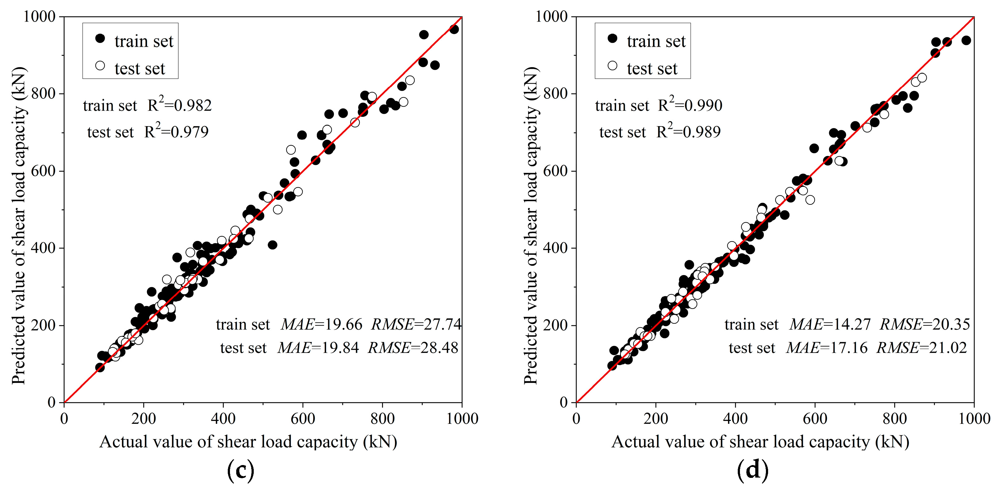
4.1. Correlation Analysis of Prediction Results and Comparison of Generalization Ability

To increase the credibility of the model evaluation, BP, PSO-BP and BWO-BP models were selected for cross-sectional comparison analysis with the PCA-BWO-BP model. The nodes of the four models at the input and output layers were 15 and 1, respectively. The number of nodes in the hidden layers was chosen after using the network training using Formula (9) and striving to minimize the training error. The final topology of the neural network identified in this paper is 15-10-1. The parameters were selected through the grid search method, and the average value of the MAE of each validation set in k-fold cross-validation was used as the objective function. The finalized parameters are taken as shown in

Table 3. Performance evaluation results of BP, PSO-BP, BWO-BP and PCA-BWO-BP algorithms.

Algorithm	Parameters
BP	η = 0.01; g = 0.001
PSO-BP	η = 0.01; g = 0.001; C1 = 2; C2 = 1; N = 40
BWO-BP	η = 0.01; g = 0.001; PP = 0.8; CR = 0.5; PM = 0.4; N = 30
PCA-BWO-BP	η = 0.01; g = 0.001; PP = 0.8; CR = 0.5; PM = 0.4; N = 30

Note: η—learning rate; g—training goal; C_i—learning factor; PC—crossover rate; PM—variance rate; PP—reproduction rate; CR—congeneric feeding rate.

.

$$h<\sqrt{(i+o)}+a$$

(9)

h: number of hidden layers; o: number of output layers; i: number of input layers; a is [0–10], and adopt constant.

In this paper, 80% of the data in the dataset were randomly selected as the training set and 20% of the data were chosen as the test set for shear load capacity prediction of reinforced concrete deep beams. Logsig serves as the neural network’s activation function from the input layer to the hidden layer, while the purlin function serves as its activation function from the hidden layer to the output layer. The default clearngdm function is a gradient descent function with momentum weights and bias learning, which can update the weights and bias of the neural network according to the gradient of the network performance and can use the momentum factor to improve learning speed and accuracy when training the neural network. The training function is the default trainlm function, which combines Newton’s method and gradient descent to improve learning speed and accuracy when training the neural network. The trained PCA-BWO-BP network model’s weights and thresholds are displayed in Appendix A. The four plots in Figure 5 show the correlation between the predicted data and the actual data of the BP, PSO-BP, BWO-BP and PCA-BWO-BP models in the training and testing stages, respectively.

It is clear that the BP neural network performs worse than the other three neural network models during the training and testing phases, demonstrating that it has the weakest generalization ability and the worst capacity for making predictions for unknowable data. Both the PSO-BP neural network and the BWO-BP neural network performed better than BP during testing, proving that the mutation and like-eating operations of the BWO algorithm and the individual and social learning operations of the PSO algorithm can enhance the BP neural network’s capacity for global search and generalization. The PCA-BWO-BP neural network outperforms other models in terms of prediction accuracy during testing, demonstrating that it is the most generalizable model.

The mean square error of the training and test sets of the PCA-BWO-BP neural network prediction process is shown in Figure 6 as a function of the number of iterations. The mean square error of the training set keeps going down during the evolution process. The test set mean square error drops to its lowest value at iteration 14, reaching 6.33 × 10⁻³, and then steadily rises at subsequent iterations, demonstrating that the iteration converges at this generation.

4.2. Prediction Evaluation and Error Analysis

Figure 7 shows a comparison of the prediction effects of the BP, PSO-BP, BWO-BP and PCA-BWO-BP models. It can be observed that the BP model’s prediction results vary considerably from the measured results, and the PSO-BP model’s forecast error was more than the BWO-BP model’s prediction error. The PCA-BWO-BP model predicted values that were closer to the actual values, and no severe outliers were identified, suggesting its excellent dependability in predicting sample data. It was also verified that the PCA method may reduce the data structure, and that the BWO algorithm’s cannibalism and mutation procedures better optimize the weights and thresholds of the BP neural network, resulting in the PCA-BWO-BP model obtaining greater generalization and data prediction capacity. As a result, the PCA-BWO-BP model can more precisely forecast the shear load capacity of reinforced concrete deep beams and may be employed efficiently in reality.

4.3. Predictive Model Performance Evaluation

In this paper, five different evaluation metrics, including absolute error (MAE), mean absolute percentage error (MAPE), root mean square error (RMSE), root mean square percentage error (RMSPE) and Nash efficiency coefficient (NS), are used, and their mathematical expressions are as follows.

$$MAE=\frac{1}{n}{\displaystyle \sum _{i=1}^n\left|x_i-p_i\right|}$$

(10)

$$MAPE=\frac{1}{n}{\displaystyle \sum _{i=1}^n\left|\frac{x_i-p_i}{x_i}\right|}\times 100\%$$

(11)

$$RMSE=\sqrt{\frac{1}{n}{\displaystyle \sum _{i=1}^n{\left(x_i-p_i\right)}^2}}$$

(12)

$$RMSPE=\frac{1}{n}\sqrt{{\displaystyle \sum _{i=1}^n{\left(\frac{x_i-p_i}{x_i}\right)}^2}}\times 100\%$$

(13)

$$NS=1-\frac{{\displaystyle {\sum }_{i=1}^n{(x_i-p_i)}^2}}{{\displaystyle {\sum }_{i=1}^n{(x_i-\overline{x})}^2}}$$

(14)

In the above Equations (10)–(14) x_i is the true value, p_i is the predicted value and x is the average of the true value, and the calculation results are shown in

Table 4. Performance evaluation results of BP, PSO-BP, BWO-BP and PCA-BWO-BP algorithms.

	MAE	MAPE (%)	RMSE	RMSPE (%)	NS
BP	32.173	8.820	42.408	1.237	0.954
PSO-BP	26.709	7.469	36.184	0.726	0.970
BWO-BP	19.846	5.767	28.485	0.606	0.979
PCA-BWO-BP	17.169	5.126	21.025	0.379	0.989

In the table: the closer the NS is to 1, the higher the confidence that the model has.

below.

The NS of the predicted shear load capacity of reinforced concrete deep beams obtained using the four prediction models, BP, PSO-BP, BWO-BP and PCA-BWO-BP, are all greater than 0.90, indicating that the four models can dig out the intrinsic relationship between member size, bottom longitudinal reinforcement, hoop reinforcement, concrete strength and shear load capacity of the reinforced concrete. The PCA-BWO-BP model has a better prediction impact in the five evaluation indexes of MAE, MAPE, RMSE, RMSP and NS. Furthermore, the predicted values of the PCA-BWO-BP model established in this research fit better with the real values, while the relative errors are less and more stable than the three models of BP, PSO-BP and BWO-BP, as shown in Table 4.

5. Conclusions

This paper adopted the principal component analysis algorithm and black widow optimization algorithm to optimize the structure of the BP neural network, in which the principal component analysis method reduces the dimension of the input variables, and the black widow optimization algorithm optimizes the weights and thresholds of the BP neural network structure. The shear load capacity of reinforced concrete deep beams was predicted using the optimal model (PCA-BWO-BP) with the three models of BP, PSO-BP and BWO-BP after reading about and gathering the shear test data of deep beams from the literature. The research results show that:

(1)

The principal component analysis method reduces the dimensionality of the input variables, which simplifies the construction of the BP network and increases its capacity for prediction.

(2)

In all evaluation metrics, the BWO-BP model performs better than the BP model, demonstrating that the black widow optimization algorithm can effectively optimize the weights and thresholds of the BP neural network, enhance the generalizability and robustness of the prediction model, and consequently, more accurately predict the shear load capacity of reinforced concrete deep beams.

(3)

The PCA-BWO-BP model outperforms the other three models with higher prediction accuracy and better stability, with a mean absolute error (MAE), mean absolute percentage error (MAPE), root mean square error (RMSE), root mean square percentage error (RMSPE) and Nash efficiency coefficient (NS) of 17.169, 5.126, 21.025, 0.379 and 0.989, respectively, in predicting the shear bearing capacity of reinforced concrete deep beams.

In the future, the PCA-BWO-BP model and the AI model can be coupled to offer helpful references for the design and assessment of reinforced concrete deep beams.

References

1. Wang, J.; Liu, J.; Zhang, G.; Jia, Y. Method for computing the shear capacity of prestressed reinforced concrete beams based on truss-arch model. Int. J. Struct. Integr. 2018, 9, 574–586. [Google Scholar] [CrossRef]
2. Russo, G.; Somma, G.; Mitri, D. Shear Strength Analysis and Prediction for Reinforced Concrete Beams without Stirrups. J. Struct. Eng. 2005, 131, 66–74. [Google Scholar] [CrossRef]
3. Zararis, P.D. Shear Compression Failure in Reinforced Concrete Deep Beams. J. Struct. Eng. 2003, 129, 544–553. [Google Scholar] [CrossRef]
4. Bekas, G.; Stavroulakis, G.E. Machine Learning and Optimality in Multi Storey Reinforced Concrete Frames. Infrastructures 2017, 2, 6. [Google Scholar] [CrossRef]
5. Kang, M.C.; Yoo, D.Y.; Gupta, R. Machine learning-based prediction for compressive and flexural strengths of steel fiber-reinforced concrete. Constr. Build. Mater. 2021, 266, 121117. [Google Scholar] [CrossRef]
6. Mansour, M.Y.; Dicleli, M.; Lee, J.Y.; Zhang, J. Predicting the shear strength of reinforced concrete beams using artificial neural networks. Eng. Struct. 2004, 26, 781–799. [Google Scholar] [CrossRef]
7. Abdalla, J.A.; Elsanosi, A.; Abdelwahab, A. Modeling and simulation of shear resistance of R/C beams using artificial neural network. J. Frankl. Inst. 2007, 344, 741–756. [Google Scholar] [CrossRef]
8. Wakjira, T.G.; Al-Hamrani, A.; Ebead, U.; Alnahhal, W. Shear capacity prediction of FRP-RC beams using single and ensenble ExPlainable Machine learning models. Compos. Struct. 2022, 287, 115381. [Google Scholar] [CrossRef]
9. Chou, J.-S.; Pham, T.; Nguyen, T.; Pham, A.-D.; Ngoc, T.N. Shear strength prediction of reinforced concrete beams by baseline, ensemble, and hybrid machine learning models. Soft Comput. 2020, 24, 3393–3411. [Google Scholar] [CrossRef]
10. Erdem, H. Prediction of the moment capacity of reinforced concrete slabs in fire using artificial neural networks. Adv. Eng. Softw. 2010, 41, 270–276. [Google Scholar] [CrossRef]
11. Koçer, M.; Öztürk, M.; Hakan Arslan, M. Determination of moment, shear and ductility capacities of spiral columns using an artificial neural network. J. Build. Eng. 2019, 26, 100878. [Google Scholar] [CrossRef]
12. Golafshani, E.M.; Rahai, A.; Sebt, M.H.; Akbarpour, H. Prediction of bond strength of spliced steel bars in concrete using artificial neural network and fuzzy logic. Constr. Build. Mater. 2012, 36, 411–418. [Google Scholar] [CrossRef]
13. Zhang, W.; Zhang, L.; Yang, J.; Hao, X.; Guan, G.; Gao, Z. An experimental modeling of cyclone separator efficiency with PCA-PSO-SVR algorithm. Powder Technol. 2019, 347, 114–124. [Google Scholar] [CrossRef]
14. Xiong, Q.; Xiong, H.; Kong, Q.; Ni, X.; Li, Y.; Yuan, C. Machine learning-driven seismic failure mode identification of reinforced concrete shear walls based on PCA feature extraction. Structures 2022, 44, 1429–1442. [Google Scholar] [CrossRef]
15. Jian, H.; Lin, Q.; Wu, J.; Fan, X.; Wang, X. Design of the color classification system for sunglass lenses using PCA-PSO-ELM. Measurement 2022, 189, 110498. [Google Scholar] [CrossRef]
16. Zhang, Y.; Gao, X.; Katayama, S. Weld appearance prediction with BP neural network improved by genetic algorithm during disk laser welding. J. Manuf. Syst. 2015, 34, 53–59. [Google Scholar] [CrossRef]
17. Yu, L.; Xie, L.; Liu, C.; Yu, S.; Guo, Y.; Yang, K. Optimization of BP neural network model by chaotic krill herd algorithm. Alex. Eng. J. 2022, 61, 9769–9777. [Google Scholar] [CrossRef]
18. Zhao, Z.; Xu, Q.; Jia, M. Improved shuffled frog leaping algorithm-based BP neural network and its application in bearing early fault diagnosis. Neural Comput. Appl. 2016, 27, 375–385. [Google Scholar] [CrossRef]
19. Bai, T.; Meng, H.; Yao, J. A forecasting method of forest pests based on the rough set and PSO-BP neural network. Neural Comput. Appl. 2014, 25, 1699–1707. [Google Scholar] [CrossRef]
20. Memar, S.; Mahdavi-Meymand, A.; Sulisz, W. Prediction of seasonal maximum wave height for unevenly spaced time series by Black Widow Optimization algorithm. Mar. Struct. 2021, 78, 103005. [Google Scholar] [CrossRef]
21. Munagala, V.K.; Jatoth, R.K. Improved fractional PI λ D μ controller for AVR system using Chaotic Black Widow algorithm. Comput. Electr. Eng. 2022, 97, 107600. [Google Scholar] [CrossRef]
22. Hayyolalam, V.; Pourhaji Kazem, A.A. Black Widow Optimization Algorithm: A novel meta-heuristic approach for solving engineering optimization problems. Eng. Appl. Artif. Intell. 2020, 87, 103249. [Google Scholar] [CrossRef]
23. Clark, A.P. Diagonal Tension in Reinforced Concrete Beams. J. Proc. 1951, 48, 145–156. [Google Scholar] [CrossRef]
24. Moody, K.G.; Viest, I.M.; Elstner, R.C.; Hognestad, E. Shear Strength of Reinforced Concrete Beams Part 1-Tests of Simple Beams. J. Proc. 1954, 51, 317–332. [Google Scholar] [CrossRef]
25. Morrow, J.; Viest, I.M. Shear Strength of Reinforced Concrete Frame Members Without Web Reinforcement. J. Proc. 1957, 53, 833–869. [Google Scholar] [CrossRef]
26. Mathey, R.G.; Watstein, D. Shear Strength of Beams Without Web Reinforcement Containing Deformed Bars of Different Yield Strengths. J. Proc. 1963, 60, 183–208. [Google Scholar] [CrossRef]
27. Smith, K.N.; Vantsiotis, A.S. Shear Strength of Deep Beams. J. Proc. 1982, 79, 201–213. [Google Scholar] [CrossRef]
28. Walravena, J.; Lehwalter, N. Size Effects in Short Beams Loaded in Shear. Struct. J. 1994, 91, 585–593. [Google Scholar] [CrossRef]
29. Tanimura, Y.; Sato, T.; Watanabe, T.; Matsuoka, S. Shear Strength of Deep Beams with Stirrups. Doboku Gakkai Ronbunshu 2004, 2004, 29–44. [Google Scholar] [CrossRef] [PubMed]
30. Quintero-Febres, C.G.; Parra-Montesinos, G.; Wight, J.K. Strength of Struts in Deep Concrete Members Designed Using Strut-and-Tie Method. Struct. J. 2006, 103, 577–586. [Google Scholar] [CrossRef]
31. Sahoo, D.K.; Sagi, M.S.V.; Singh, B.; Bhargava, P. Effect of Detailing of Web Reinforcement on the Behavior of Bottle-shaped Struts. J. Adv. Concr. Technol. 2010, 8, 303–314. [Google Scholar] [CrossRef]
Figure 1. Basic principle and schematic procedure of PCA.
Buildings 13 01395 g001
Figure 2. BP neural net. Note: wij and θj denote the weights from the input layer to the hidden layer and from the hidden layer to the output layer, respectively; vik and ok are the thresholds of the hidden layer and the output layer, respectively.
Buildings 13 01395 g002
Figure 3. Black widow optimization algorithm schematic.
Buildings 13 01395 g003
Figure 4. Flow chart of PCA-BWO-BP model.
Buildings 13 01395 g004
Figure 5. The correlation between the prediction output data and the actual output data at the three stages of training, verification and testing. (a) BP; (b) PSO-BP; (c) BWO-BP; (d) PCA-BWO-BP.
Buildings 13 01395 g005aBuildings 13 01395 g005b
Figure 6. PCA-BWO-BP iteration curve.
Buildings 13 01395 g006
Figure 7. Comparison of prediction results of BP, PSO-BP, BWO-BP and PCA-BWO-BP.
Buildings 13 01395 g007