Numerical Evaluation of Transverse Steel Connector Strengthening Effect on the Behavior of Rubble Stone Masonry Walls under Compression Using a Particle Model

Abstract

The structural rehabilitation of historic/traditional rubble masonry wall constructions requires consolidation and retrofitting solutions to be employed in order to withstand dynamic loads, high vertical loads, and differential settlements. One of these strengthening techniques is based on the use of steel bar connectors perpendicular to the wall, considered individually or integrated into more complex strengthening techniques. The aim of this study is to evaluate numerically the strengthening effect of transverse steel connectors on rubble masonry walls. With this purpose, a 2D particle-reinforced model (2D-PMR) was devised and applied to model uniaxial compression tests. The results presented show that predictions calculated using the proposed 2D-PMR model are very close to known experimental results, particularly in the corresponding failure modes, the increase of the maximum uniaxial compression value, and ductility. Parametric studies are also conducted by varying the diameter of the steel bars and the level of strengthening to assess the influence of the bar-bond effect and lateral plates. The presented parametric numerical studies show that (i) a two-level strengthening solution guarantees a similar response to the three-level strengthening solution adopted in the experiments; (ii) it is not relevant to apply a grout injection during the application process of the steel connectors if lateral plates are adopted; and (iii) the 2D-PMR model can be used in the definition of the steel bar diameter and properties; as shown, a smaller (8 mm) bar diameter predicts a similar strengthening effect to the (12 mm) bar size adopted in the experiments. Given the performance of the proposed 2D-PMR model, further work is underway that will allow the 2D-PMR model to numerically assess other reinforcement techniques, namely, reinforced micro-concrete layers and textile reinforced mortar.

1. Introduction

Ancient masonry buildings represent a significant percentage of the historic and architectural heritage all over the world, including regions prone to seismic hazards. According to [1], in Portugal, ancient masonry buildings account for around 50% of the built heritage, many of which are classified as heritage sites (monuments, palaces, convents, castles, churches, etc.).

In recent decades, there has been a growing interest in restoring, rehabilitating, and preserving historic cities and their existing stone masonry buildings. It is widely acknowledged that the stone masonry walls of ancient structures have reasonable resistance to vertical loads but considerably lower shear and tensile strength. To improve the behavior of these walls, lateral stability and resistance to gravitational actions must be ensured through the implementation of straightening solutions [2,3,4,5,6]. A state-of-the-art review on seismic upgrading of existing masonry structures, including rubble stone masonry walls, is presented in [7]. An extensive experimental campaign was conducted on multi-leaf, low-strength, natural stone masonry specimens using various techniques [8]. The experimental findings provide a better understanding of the behaviors of ordinary and strengthened rubble masonry walls [2,9,10], and quantify the increase in strength and ductility of the studied solutions.

One of the strengthening techniques involves the use of steel bar connectors perpendicular to the wall, either individually or as part of more complex rehabilitation techniques [6]. This technique provides transverse confinement, preventing detachments of the masonry, particularly the stones, caused by high compression loads and improving the global mechanical characteristics, including compression and shear strength. However, to optimize the reinforcement solutions, numerical analyses are useful in the design of those solutions. Studies on the effectiveness of strengthening solutions of multi-leaf masonry walls based on transverse steel connectors are also reported in [11].

Existing rubble stone masonry is notoriously complex to model accurately due to its heterogeneity, uncertainty in material properties, including nonlinear behavior, and geometric unevenness of the stones’ size. The masonry analysis can be performed at the macro scale or micro scale. In a macro-modeling approach [12,13], which is suitable for large-scale analysis, the masonry wall is considered a single homogenized continuum and is typically modeled within a finite element (FEM) framework. In a micro-modeling approach, each component is individually modeled at the real scale, including the stone–brick, the mortar, and in many cases, the stone–mortar interface. One drawback of this approach is the intensive computational effort that is required, limiting its application for the analysis of large structures. Despite this, the micro-modeling approach offers a significant advantage in capturing localized cracking patterns as a real discontinuity, thus allowing for a better understanding of the brittle failure processes that occur in masonry structures. A variety of numerical methods can be adopted within the micro-modeling approach. The FEM with joints can be used to model the stones and joints [14]. A polygonal discrete element method (DEM) can be used to model rigid or flexible block interactions of dry and mortared joints [15,16]. A rigid circular particle DEM model was proposed for rubble stone masonry in [17]. The simultaneous use of FEM and DEM techniques proposed in [18,19] combines the advantages of both the finite and discrete element methods. The discontinuous strain analysis (DDA) approach, as proposed in [20], is also able to model large block displacements, such as the DEM-based approaches.

In this paper, a detailed micro-modeling strategy based on a particle model (2D-PM) [21,22,23] is adopted, which is known to successfully model the complex macroscopic failure with simple constitutive models by taking into account the material structure at the grain scale. This approach has been adopted by the authors in the modeling of traditional rubble stone masonry walls under uniaxial compression loading [24]. After calibrating the contact parameters using known mortar and stone experimental data, the 2D-MP model is capable of predicting and representing the elastic response, the process of crack formation, propagation in rubble masonry walls, and the peak load value in uniaxial compression based on simple interaction models [24]. The 2D-PM model is also an excellent framework to generate the heterogeneity that is present in rubble masonry walls. The high computational effort characteristic of PM models can be reduced by adopting a hybrid DEM-FEM model as proposed in [19].

The numerical models developed in this paper are based on experimental studies conducted by Pinho et al. [2,6,9,10] on rubble stone masonry specimens constructed with hydrated air lime mortar and strengthened by simple transverse confinement. The study proposes a 2D-PM reinforced model (2D-PMR) in which the steel connectors are modeled using FEM-based frame elements, and the stone–steel and mortar–steel interactions through the grout, are modeled by means of a particle-bar contact interface. The proposed 2D-PMR numerical model, which is implemented in the parmac2D [25] application, is used to evaluate the response of the reference and three-level strengthened wall specimens used in the experimental campaign.

The numerical results presented demonstrate that the proposed 2D-PM reinforced model can predict the improvement in terms of strength and ductility, crack growth, and reduction in horizontal detachments that occur during the experimental tests of rubble stone masonry walls strengthened with transverse confinement. Hence, the proposed numerical scheme enables the 2D-PMR model to simulate the effect of steel-based transverse confinement on rubble masonry walls.

Several parametric studies were carried out using the 2D-PM reinforced numerical model regarding the (a) strengthening scheme, (b) steel bar diameter, (c) bar-wall element bonds, and (d) lateral steel plate influence. A higher peak strength increase is predicted with a strong particle/bar bond approach (50%) that is slightly higher than the average increase in strength (47%) identified experimentally. A weak particle/bar bond approach predicts a lower peak strength increase (20%). When a weak particle/bar bond approach (WB) was used, a two-level reinforcement solution (four steel bars) predicted a higher peak strength than the peak strength predicted with the three-level reinforcement solution used in the experiment (five steel bars). The presented numerical results clearly demonstrate that when plates are placed at the lateral faces of the walls, the bond between the connectors and wall components is not significant, indicating that more cost-effective strengthening solutions can be adopted without the need for mortar filling and drilling holes larger than the steel bar diameters. The importance of the lateral plates in the strengthening mechanism is also highlighted. When the steel plates are not present, the connector/wall bond is important in order for the strengthening mechanism to be effective. A significant increase in peak strength and ductility is predicted only under the strong bond assumption when lateral plates are not present.

Finally, the presented parametric studies clearly show that the proposed 2D-PMR model can be adopted in the development of reinforcement solutions by simple transverse confinement, namely in the definition of bar characteristics, positioning, quantification, and assessment of the relevance of the grout injection in the application process of the steel connectors.

2. Modeling of the Masonry by a Particle Model

The modeling approach is based on the assumption that the constituent elements of the masonry structure (stones and mortar) consist of a skeleton of aggregates of various dimensions in direct contact with cohesive connections that enable the aggregates to withstand tensile forces. Unlike FE-based micro-modeling approaches, which require complex cohesive contact models and face convergence issues under cycling loading and large displacement [26], particle models are capable of predicting complex macroscopic failure phenomena with simple constitutive models by directly taking into account the physical particle interactions and material randomness associated with the grain structure of the wall’s components: stone units, mortar, and reinforcement elements. Additionally, particle models are suitable for large displacement analysis and cyclic loading and can generate complex numerical models that are representative of rubble stone masonry.

Previous studies conducted by the authors on URM specimens [24,27] have demonstrated that particle models can be effectively utilized as a predictive tool for rubble-stone masonry walls constructed with hydrated air lime mortar [2,10] under uniaxial compressive loading conditions. As demonstrated in [24,27], good agreement can be achieved with stone masonry wall behavior, including elastic response, peak strength, and ductility, provided that the calibration of the contact parameters is based on experimental data of the components obtained from laboratory tests.

In the study presented in [24], three important findings are reported: (i) the lateral numerical model can reproduce the URM peak strength and overall mechanical behavior; (ii) a coarser mortar discretization can be employed without affecting the quality of the numerical predictions; and (iii) a maximum contact compressive yielding stress is necessary to adopt under compression due to the heterogeneity of URM. These findings are encouraging for the use of the 2D-PM model in evaluating the efficacy of transverse reinforcement strengthening systems.

2.1. Particle Model Formulation

In the particle model (PM) formulation, the constituent materials of the masonry are represented by particles that interact with each other through contact interfaces. In 2D-PM models, particles are usually adopted with circular geometry. The numerical solution is obtained by sequentially applying Newton’s second law to calculate the new particle positions and velocities, and force–displacement law to determine the forces at each contact. The equations of motion, including non-viscous local damping, are given by Equations (1) and (2):

$$\begin{array}{c}\hfill F_i\left(t\right)+F_i^d\left(t\right)=m{\ddot{x}}_i\left(t\right)\end{array}$$

(1)

$$\begin{array}{c}\hfill M_3\left(t\right)+M_3^d\left(t\right)=I{\dot{\omega }}_3\left(t\right)\end{array}$$

(2)

where at time t, $F_i\left(t\right)$ is the force vector and $M_3\left(t\right)$ corresponds to the applied moment; $F_i^d\left(t\right)$ and $M_3^d\left(t\right)$ are the force vector and moment associated with the local non-viscous damping [24]; ${\ddot{x}}_i$ is the acceleration, ${\dot{\omega }}_3$ is the angular acceleration of the particle; $i=1,2$ indicates the global x and y directions; and m and I correspond to the particle’s mass and inertia of the spherical particle.

The integration of the equation of motion is performed explicitly, using the central differences method [17]. In each step, the increments of the normal force, $\Delta F_n$, and shear force, $\Delta F_s$, at each contact point, are determined according to a linear force–displacement relationship, (3) and (4):

$$\begin{array}{cc}\hfill & \Delta F_n^{\left[C\right]}=k_n\Delta x_n^{\left[C\right]}\end{array}$$

(3)

$$\begin{array}{cc}\hfill & \Delta F_s^{\left[C\right]}=k_s\Delta x_s^{\left[C\right]}\end{array}$$

(4)

where $\Delta x_n^{\left[C\right]}$ and $\Delta x_s^{\left[C\right]}$ represent the displacement increments at the contact point on the normal and shear directions and $k_n$ and $k_s$ represent the normal and shear contact stiffness, respectively.

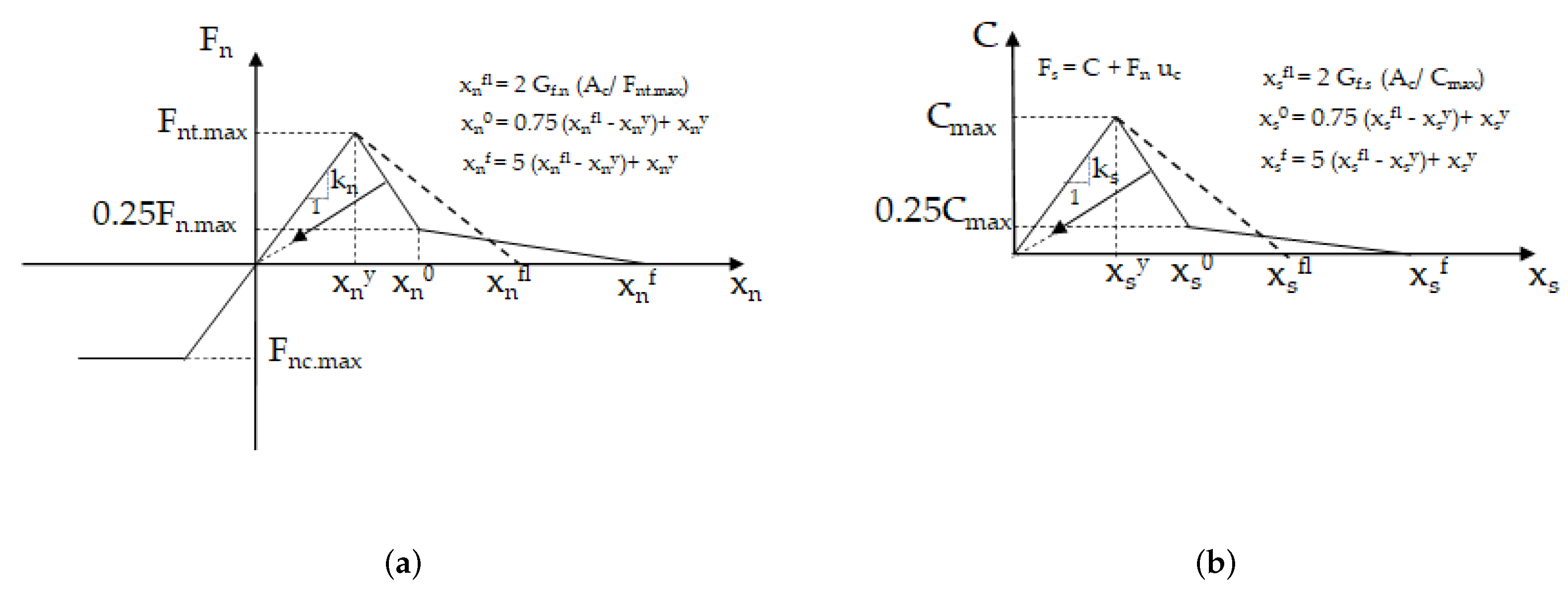
2.2. Contact Stiffness and Contact Strength

In the numerical simulations that are carried out, the stiffness of the contact in the normal and shear directions are given by Expressions (5) and (6):

$$\begin{array}{cc}\hfill & k_n=\overline{E}{A}_c/d\end{array}$$

(5)

$$\begin{array}{cc}\hfill & k_s=\alpha k_n\end{array}$$

(6)

where $\overline{E}$ is the modulus of elasticity of the equivalent continuous material; d is the distance between the gravity centers of the particles in contact; $A_c$ is the contact area; and $\alpha$ relates the normal and the shear contact stiffness.

The maximum contact tensile strength, $F_{nt,max}$, the maximum cohesive force, $C_{max}$, and the maximum contact compressive strength, $F_{nc,max}$, are given as functions of the adopted maximum tensile stress, ${\sigma }_{nt,c}$, maximum cohesion stress, ${\tau }_c$, maximum compressive stress, ${\sigma }_{nc,c}$ and by the contact area, $A_c$, according to Expressions (7)–(9):

$$\begin{array}{cc}\hfill & F_{nt,max}={\sigma }_{nt,c}{A}_c\end{array}$$

(7)

$$\begin{array}{cc}\hfill & C_{max}={\tau }_c{A}_c\end{array}$$

(8)

$$\begin{array}{cc}\hfill & F_{nc,max}={\sigma }_{nc,c}{A}_c\end{array}$$

(9)

In the normal direction, under tensile loading and in the shear direction, a damage model with bilinear softening is adopted for the contact [17], shown in Figure 1. In the normal direction, under compressive loading, a yield plateau is adopted, given by Equation (9). As pointed out in previous studies [24], due to the heterogeneity present in ancient masonry walls built with hydrated air lime mortar, it is necessary to adopt a maximum contact compressive strength value.

The adopted bilinear softening contact model, under tensile loading and shear loading, requires the definition of the contact tensile fracture energy, $G_{f,n}$, and of the contact shear fracture energy $G_{f,s}$. The maximum values of the tensile strength and cohesion are reduced according to the total damage value, which is defined by the sum of the tensile and shear damage. In each direction, the damage value is defined as a function of the maximum contact displacement in that direction. When the contact damage reaches the value of 1, the contact is considered to be cracked, only being able to work in compression under pure friction. For more details on the 2D-PM formulation, the reader is referred to [24].

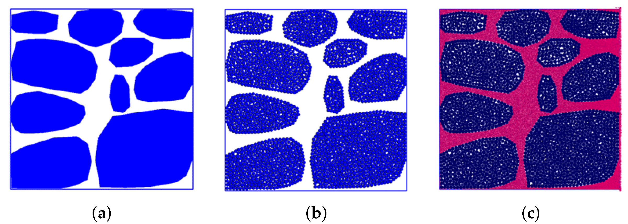
2.3. Particle Model Generation

The numerical model for a stone masonry structure using the 2D-PM is created by generating a particle assembly for each stone unit, and by generating a particle assembly inside the elements that represent the mortar. The main steps of the PM generation are illustrated in Figure 2.

The first step in this process is the identification of the arrangement and geometry of the stones in the masonry wall, Figure 2a, followed by the discretization of the space corresponding to the interior of each stone with inner particles, Figure 2b. Then, the laying mortar, corresponding to the external domain of each stone, is further discretized with particles, Figure 2c.

The contacts are defined based on the Voronoi–Laguerre tessellation of the gravity centers of each circular particle [22]. In this way, an approximate polygonal geometry is incorporated in each particle, improving the performance of the adopted 2D-PM model when compared to traditional PM models. More details can be found in [22].

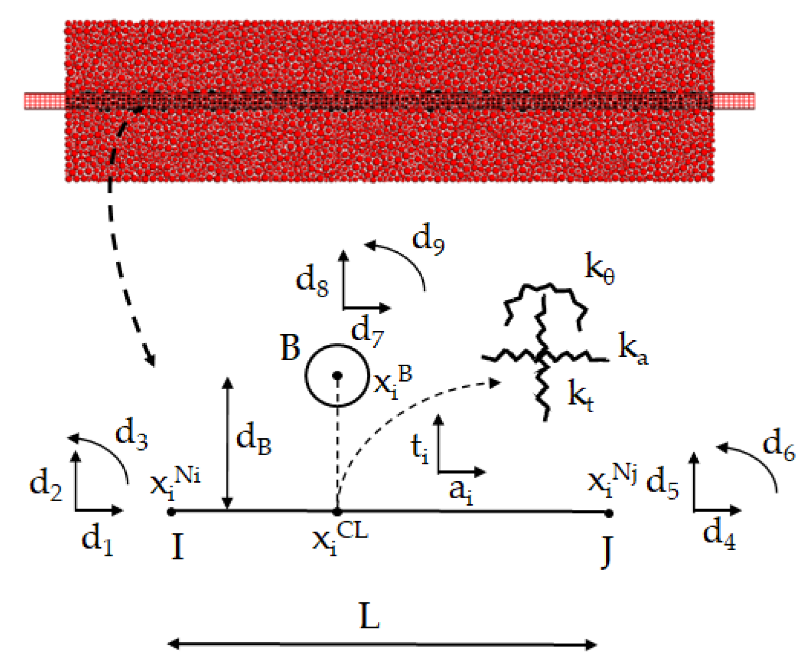
2.4. Steel Connectors and Steel Bar-Particle Interaction Model

The steel connectors are modeled through plane frame finite elements with three degrees of freedom per node. The traditional shape functions (N) and shape function derivatives ($dN$) are used to set the plane frame displacement field, given the nodal values [25]. The numerical analysis employs an elastic-perfectly plastic stress–strain relationship for the plane frame elements representing the steel bars.

The interaction between a bar, discretized using plane frame finite elements, and a given particle representing each masonry wall component (mortar or stone) occurs through a given contact interface, as proposed in [25]. For contact detection purposes (see Figure 3), it is assumed that the geometry of the plane frame element can be approximated by the linear segment connecting the plane frame nodes.

At a given simulation instant, the plane frame length, L, and the plane frame axial direction, ${\mathbf{a}}_i$, are given by Equations (10) and (11):

$$\begin{array}{ccc}\hfill L& =& \sqrt{({\mathbf{x}}_{\mathbf{i}}^{N_j}-{\mathbf{x}}_{\mathbf{i}}^{N_i})({\mathbf{x}}_{\mathbf{i}}^{N_j}-{\mathbf{x}}_{\mathbf{i}}^{N_i})}\hfill \end{array}$$

(10)

$$\begin{array}{ccc}\hfill {\mathbf{a}}_{\mathbf{i}}& =& \frac{{\mathbf{x}}_{\mathbf{i}}^{N_j}-{\mathbf{x}}_{\mathbf{i}}^{N_i}}{L}\hfill \end{array}$$

(11)

The transverse/normal direction of the plane frame element, ${\mathbf{t}}_{\mathbf{i}}$, is defined based on the bar’s axial direction through $t=(-a_2,a_1)$. It is assumed that the contact point location ${\mathbf{x}}_{\mathbf{i}}^{CL}$, hereafter called the interface location, through which a particle interacts with a given plane frame element, is defined at a given instant by the plane frame element normal and the particle centre of gravity. The location of the contact interface is given by the orthogonal projection of the particle’s centre onto the plane frame segment, as illustrated in Figure 3.

The interface velocity is defined as the relative velocity of the two entities at the contact interface. The relative velocity of the plane frame element $\left({\Phi }^2\right)$ relative to the particle $\left({\Phi }^1\right)$ at the contact interface is given by Equation (12):

$${\dot{\mathbf{x}}}_{\mathbf{i}}^{CL}={\left({\dot{\mathbf{x}}}_{\mathbf{i}}^{CL}\right)}_{{\Phi }^2}-{\left({\dot{\mathbf{x}}}_{\mathbf{i}}^{CL}\right)}_{{\Phi }^1}$$

(12)

where ${\dot{\mathbf{x}}}_{\mathbf{i}}^{CL}$ is the contact interface velocity, and ${\left({\dot{\mathbf{x}}}_{\mathbf{i}}^{CL}\right)}_{{\Phi }^i}$ is the velocity of the entity ${\Phi }^i$ at the contact interface. The velocity of particle B at the contact interface ${\dot{\mathbf{x}}}_{\mathbf{i}}^{CB}$ is defined through the traditional DEM formulation [25]. The velocity of the plane frame element at the contact interface ${\dot{\mathbf{x}}}_{\mathbf{i}}^{CF}$ follows the formulation proposed in [25]. For a given node h, the nodal translational velocities in the plane frame element reference axes are defined using Expressions (13) and (14):

$$\begin{array}{ccc}\hfill {\dot{x}}_a^{Nh}& =& {\dot{\mathbf{x}}}_{\mathbf{i}}^{Nh}{\mathbf{a}}_{\mathbf{i}}\hfill \end{array}$$

(13)

$$\begin{array}{ccc}\hfill {\dot{x}}_t^{Nh}& =& {\dot{\mathbf{x}}}_{\mathbf{i}}^{Nh}{\mathbf{t}}_{\mathbf{i}}\hfill \end{array}$$

(14)

For the plane frame element, it is also necessary to define the rotational velocity of the rigid body, ${\omega }_3^{RB}$, according to Equation (15):

$${\omega }_3^{\left[RB\right]}=\frac{{ϵ}_{3jk}{\mathbf{a}}_{\mathbf{j}}{\mathbf{a}}_{\mathbf{k},\mathbf{old}}}{{\Delta }_t}$$

(15)

where ${ϵ}_{3jk}{\mathbf{a}}_{\mathbf{j}}{\mathbf{a}}_{\mathbf{k},\mathbf{old}}$ represents the external product of the current and previous axial directions of the plane frame element. The rotational velocity of node h relative to the plane frame element axial axis, ${\omega }_3^{R,Nh}$, can be defined through (16):

$${\omega }_3^{R,Nh}={\omega }_3^{Nh}-{\omega }_3^{RB}$$

(16)

where ${\omega }_3^{Nh}$ is the rotational velocity of node h. Given the shape functions for each nodal point and the translational and rotational velocities, it is possible to define the velocity of the plane frame element at the contact interface ${\dot{\mathbf{x}}}_{\mathbf{i}}^{CF}$. The axial velocity ${\dot{x}}_a^{CF}$ and the transverse velocity ${\dot{x}}_t^{CF}$ of the plane frame element at the contact interface are defined through Equations (17) and (18):

$$\begin{array}{ccc}\hfill {\dot{x}}_a^{CF}& =& {\dot{x}}_a^{Ni}{N}_1+{\dot{x}}_a^{Nj}{N}_4\hfill \end{array}$$

(17)

$$\begin{array}{ccc}\hfill {\dot{x}}_t^{CF}& =& {\dot{x}}_t^{Ni}{N}_2+{\dot{x}}_t^{Nj}{N}_5+{\omega }_3^{R,Ni}{N}_3+{\omega }_3^{R,Nj}{N}_6\hfill \end{array}$$

(18)

where $N_i$ represents the nodal shape functions associated with the degrees of freedom of the plane frame element nodal points; Figure 3. The rotational velocity of the plane frame element at the contact interface ${\omega }_3^{CF}$ is defined through (19):

$${\omega }_3^{CF}={\dot{x}}_t^{Ni}d{N}_2+{\dot{x}}_t^{Nj}d{N}_5+{\omega }_3^{R,Ni}d{N}_3+{\omega }_3^{R,Nj}d{N}_6+{\omega }_3^{\left[RB\right]}$$

(19)

The translational contact velocity of the plane frame element at the contact interface is given in global coordinates by (20):

$${\dot{x}}^{CL}={\dot{x}}_a^{CL}{\mathbf{a}}_{\mathbf{i}}+{\dot{x}}_t^{CL}{\mathbf{t}}_{\mathbf{i}}$$

(20)

The increment of the interface displacement $\Delta {\mathbf{x}}_{\mathbf{i}}^{CL}$ for a time increment of ${\Delta }_t$ is given by (21):

$$\Delta {\mathbf{x}}_{\mathbf{i}}^{CL}={\dot{\mathbf{x}}}_{\mathbf{i}}^{CL}{\Delta }_t$$

(21)

The displacement increment at the contact point can be decomposed into its axial, $\Delta {\mathbf{x}}_{\mathbf{ai}}^{CL}$, and transverse, $\Delta x_t^{CL}$ components, as given by Equations (22) and (23):

$$\begin{array}{ccc}\hfill \Delta x_t^{CL}& =& \Delta {\mathbf{x}}_{\mathbf{i}}^{CL}{\mathbf{t}}_{\mathbf{i}}\hfill \end{array}$$

(22)

$$\begin{array}{ccc}\hfill \Delta {\mathbf{x}}_{\mathbf{ai}}^{CL}& =& \Delta {\mathbf{x}}_{\mathbf{i}}^{CL}-\Delta x_t^{CL}{\mathbf{t}}_{\mathbf{i}}\hfill \end{array}$$

(23)

The contact force increments are obtained using the following linear incremental laws, (24) and (25):

$$\begin{array}{ccc}\hfill \Delta F_t^{CL}& =& k_t\Delta x_t^{CL}\hfill \end{array}$$

(24)

$$\begin{array}{ccc}\hfill \Delta {\mathbf{F}}_{\mathbf{ai}}^{CL}& =& k_a\Delta {\mathbf{x}}_{\mathbf{ai}}^{CL}\hfill \end{array}$$

(25)

where $\Delta F_t^{CL}$ is the increment of the transverse contact force given as a scalar, $k_t$ is the transverse interface stiffness that relates transverse displacement increments with transverse interface force increments, and $k_a$ is the axial contact stiffness. The rotation increment at the contact interface $\Delta {\theta }_3^{CL}$ for a time increment of ${\Delta }_t$ is given by (26):

$$\Delta {\theta }_3^{CL}=({\omega }_3^{\left[{\Phi }^2\right]}-{\omega }_3^{\left[{\Phi }^1\right]}){\Delta }_t={\omega }_3^{\left[CF\right]}-{\omega }_3^{\left[B\right]}$$

(26)

where ${\omega }_3^{\left[{\Phi }^i\right]}$ is the rotational velocity of entity ${\Phi }^i$ at the contact interface. The contact moment increment $\Delta M_3^{\left[CL\right]}$ is obtained using the linear incremental law given by (27):

$$\Delta M_3^{CL}=k_{\theta }\Delta {\theta }_3^{CL}$$

(27)

where $k_{\theta }$ is the rotational contact spring stiffness. The transverse, the axial forces, and the contact moment acting at the interface are then updated by applying Equations (28)–(30):

$$\begin{array}{ccc}\hfill F_t^{CL}& =& F_t^{CL,old}+\Delta F_t^{CL}\hfill \end{array}$$

(28)

$$\begin{array}{ccc}\hfill {\mathbf{F}}_{\mathbf{ai}}^{CL}& =& {\mathbf{F}}_{\mathbf{ai}}^{CL,old}+\Delta {\mathbf{F}}_{\mathbf{ai}}^{\left[CL\right]}\hfill \end{array}$$

(29)

$$\begin{array}{ccc}\hfill M_3^{\left[CL\right]}& =& M_3^{[CL,old]}+\Delta M_3^{\left[CL\right]}\hfill \end{array}$$

(30)

where $F_t^{CL,old}$ (scalar) is the previous transverse interface force, vector ${\mathbf{F}}_{\mathbf{ai}}^{CL,old}$ is the previous axial interface force, and $M_3^{[CL,old]}$ (scalar) is the previously stored value of the contact moment. The contact interface force ${\mathbf{F}}_{\mathbf{i}}^{CL}$ acting at the interface location is defined by Equation (31):

$${\mathbf{F}}_{\mathbf{i}}^{CL}=F_t^{CL}{\mathbf{t}}_{\mathbf{i}}+{\mathbf{F}}_{\mathbf{ai}}^{CL}$$

(31)

The contribution of the interface force and moment to the resulting force ${\mathbf{F}}_{\mathbf{i}}^{\left[{\Phi }_1\right]}$ and moment $M_3^{\left[{\Phi }_1\right]}$ applied at particle B in contact is obtained by applying Expressions (32) and (33):

$$\begin{array}{ccc}\hfill {\mathbf{F}}_{\mathbf{i}}^{\left[{\Phi }_1\right]}& =& {\mathbf{F}}_{\mathbf{i}}^{\left[{\Phi }_1\right]}+{\mathbf{F}}_{\mathbf{i}}^{\left[CL\right]}\hfill \end{array}$$

(32)

$$\begin{array}{ccc}\hfill M_3^{\left[{\Phi }_1\right]}& =& M_3^{\left[{\Phi }_1\right]}+{ϵ}_{3jk}({\mathbf{x}}_{\mathbf{j}}^{\left[CL\right]}-{\mathbf{x}}_{\mathbf{j}}^{\left[{\Phi }^1\right]}){\mathbf{F}}_{\mathbf{k}}^{\left[CL\right]}+M_3^{\left[CL\right]}\hfill \end{array}$$

(33)

The contact interface force is distributed to the nodes according to the plane frame shape functions and the contact interface moment is distributed using the shape function derivatives. Prior to the use of the shape functions and the shape function derivatives, it is necessary to define the contact interface force in the reference axes, as shown in Equations (34) and (35):

$$\begin{array}{ccc}\hfill F_a^{\left[CL\right]}& =& {\mathbf{F}}_{\mathbf{i}}^{CL}{\mathbf{a}}_{\mathbf{i}}\hfill \end{array}$$

(34)

$$\begin{array}{ccc}\hfill F_t^{\left[CL\right]}& =& {\mathbf{F}}_{\mathbf{i}}^{CL}{\mathbf{t}}_{\mathbf{i}}\hfill \end{array}$$

(35)

Given the interface axial force, it is possible to define the contributions to each axial force node of the plane frame element according to Equations (36) and (37):

$$\begin{array}{ccc}\hfill F_a^{\left[CNi\right]}& =& F_a^{CL}{N}_1\hfill \end{array}$$

(36)

$$\begin{array}{ccc}\hfill F_a^{\left[CNj\right]}& =& F_a^{CL}{N}_4\hfill \end{array}$$

(37)

The contributions to the nodal transverse forces are defined by (38) and (39):

$$\begin{array}{ccc}\hfill F_t^{\left[CNi\right]}& =& F_t^{CL}{N}_2+M_3^{\left[CL\right]}d{N}_2\hfill \end{array}$$

(38)

$$\begin{array}{ccc}\hfill F_t^{\left[CNj\right]}& =& F_t^{CL}{N}_5+M_3^{\left[CL\right]}d{N}_5\hfill \end{array}$$

(39)

The moments applied at the nodal points are set, taking into account the transverse interface force; Equations (40) and (41):

$$\begin{array}{ccc}\hfill M_3^{\left[CNi\right]}& =& F_t^{CL}{N}_3+M_3^{\left[CL\right]}d{N}_3\hfill \end{array}$$

(40)

$$\begin{array}{ccc}\hfill M_3^{\left[CNj\right]}& =& F_t^{CL}{N}_6+M_3^{\left[CL\right]}d{N}_6\hfill \end{array}$$

(41)

Given the normal and transverse forces applied at a given node h, it is possible to define the interface force contribution, in vector form, using global coordinates, (42):

$${\mathbf{F}}_{\mathbf{i}}^{CNh}=F_t^{\left[CNh\right]}{\mathbf{t}}_{\mathbf{h}}+F_a^{\left[CNh\right]}{\mathbf{a}}_{\mathbf{i}}$$

(42)

The contribution of the interface force and moment to the resulting force ${\mathbf{F}}_{\mathbf{i}}^{\left[Nh\right]}$ and moment $M_3^{\left[Nh\right]}$ applied at node h is obtained according to Expressions (43) and (44):

$$\begin{array}{ccc}\hfill {\mathbf{F}}_{\mathbf{i}}^{Nh}& =& {\mathbf{F}}_{\mathbf{i}}^{\left[Nh\right]}-{\mathbf{F}}_{\mathbf{i}}^{CNh}\hfill \end{array}$$

(43)

$$\begin{array}{ccc}\hfill M_3^{\left[Nh\right]}& =& M_3^{\left[Nh\right]}-M_3^{\left[CNh\right]}\hfill \end{array}$$

(44)

The force–displacement law is applied to the identified plane frame finite element/particle interfaces. The applied forces are then used to define the new particle and the new node positions. A given particle is only allowed to interact with one finite element of the several used to model a given steel bar. The contact interface element stiffness matrix $\left[k^e\right]$ in terms of particle and nodal displacements for a reference plane passing through the transverse to plane frame element ${\mathbf{t}}_{\mathbf{i}}=(t_1,t_2)$ is defined as follows (Equation (45)):

$$\left[\begin{array}{ccccccccc}{k}_a{N}_{11}& 0& 0& k_a{N}_{41}& 0& 0& -k_a{N}_1& 0& k_a{N}_1{d}_B\\ 0& k_t{N}_{22}+k_{\theta }{N}_{22}^{{}^{\prime }}& k_t{N}_{32}+k_{\theta }{N}_{32}^{{}^{\prime }}& 0& k_t{N}_{52}+k_{\theta }{N}_{52}^{{}^{\prime }}& k_t{N}_{62}+k_{\theta }{N}_{62}^{{}^{\prime }}& 0& -k_t{N}_2& -k_{\theta }{N}_2^{{}^{\prime }}\\ 0& k_t{N}_{23}+k_{\theta }{N}_{23}^{{}^{\prime }}& k_t{N}_{33}+k_{\theta }{N}_{33}^{{}^{\prime }}& 0& k_t{N}_{53}+k_{\theta }{N}_{53}^{{}^{\prime }}& k_t{N}_{63}+k_{\theta }{N}_{63}^{{}^{\prime }}& 0& -k_t{N}_3& -k_{\theta }{N}_3^{{}^{\prime }}\\ k_a{N}_{14}& 0& 0& k_a{N}_{44}& 0& 0& -k_a{N}_4& 0& k_a{N}_4{d}_B\\ 0& k_t{N}_{25}+k_{\theta }{N}_{25}^{{}^{\prime }}& k_t{N}_{35}+k_{\theta }{N}_{35}^{{}^{\prime }}& 0& k_t{N}_{55}+k_{\theta }{N}_{55}^{{}^{\prime }}& k_t{N}_{65}+k_{\theta }{N}_{65}^{{}^{\prime }}& 0& -k_t{N}_5& -k_{\theta }{N}_5^{{}^{\prime }}\\ 0& k_t{N}_{26}+k_{\theta }{N}_{26}^{{}^{\prime }}& k_t{N}_{36}+k_{\theta }{N}_{36}^{{}^{\prime }}& 0& k_t{N}_{56}+k_{\theta }{N}_{56}^{{}^{\prime }}& k_t{N}_{66}+k_{\theta }{N}_{66}^{{}^{\prime }}& 0& -k_t{N}_6& -k_{\theta }{N}_6^{{}^{\prime }}\\ -k_a{N}_1& 0& 0& -k_a{N}_4& 0& 0& k_a& 0& -k_a{d}_B\\ 0& -k_t{N}_2& -k_t{N}_3& 0& -k_t{N}_5& -k_t{N}_6& 0& k_t& 0\\ k_a{N}_1{d}_B& -k_{\theta }{N}_2^{{}^{\prime }}& -k_{\theta }{N}_3^{{}^{\prime }}& -k_a{N}_4{d}_B& -k_{\theta }{N}_5^{{}^{\prime }}& -k_{\theta }{N}_6^{{}^{\prime }}& -k_a{d}_B& 0& k_a{d}_B^2+k_{\theta }\end{array}\right]$$

(45)

where $k_a$, $k_t$, and $k_a$ are, respectively, the contact interface axial, transverse stiffness, and rotational stiffness, $d_B=\parallel {\mathbf{x}}_{\mathbf{i}}^{\left[B\right]}-{\mathbf{x}}_{\mathbf{i}}^{CL}\parallel$ represents the Euclidean norm of the corresponding vectors, ${\mathbf{x}}_{\mathbf{i}}^B$ is the location of the center of gravity of particle B, ${\mathbf{x}}_{\mathbf{i}}^{CL}$ is the contact interface location, $N_a$ is the shape function evaluated at the interface location for dof a, $N_a^{{}^{\prime }}$ is the shape function derivative evaluated at the interface location for dof a, $N_{ab}=N_a{N}_b$ is the product of the shape functions evaluated at the interface location for dof a and dof b, and $N_{ab}^{{}^{\prime }}=N_a^{{}^{\prime }}{N}_b^{{}^{\prime }}$ is the product of the shape function derivatives evaluated at the interface location for dof a and dof b.

In order to define the critical timestep or apply a density scaling scheme, it is necessary to establish an upper bound for the translation and rotational stiffness of both the particle and the nodal points. Based on the global stiffness matrix of the contact interface and by applying Gerschgorin’s theorem to the uncoupled interface matrix, an upper bound for the translation and rotational stiffness of the particle, which does not take into consideration the interface orientation, can be defined according to [25], by Equations (46) and (47):

$$\begin{array}{ccc}\hfill k_t^{particle}& =& 2(k_a+k_t)\hfill \end{array}$$

(46)

$$\begin{array}{ccc}\hfill k_{\theta }^{particle}& =& k_a{d}_B^2+k_{\theta }\left(\right|N_3^{{}^{\prime }}|+|N_5^{{}^{\prime }}|+1)+k_a{d}_B^2\hfill \end{array}$$

(47)

An upper bound for the translational and rotational stiffness of each nodal point of the plane frame element, which does not take into consideration the interface orientation, can be defined by Equations (48) to (51):

$$\begin{array}{ccc}\hfill k_t^{Nod{e}_i}& =& 2k_a{N}_1+2k_a{N}_2+k_{\theta }{N}_{22}^{{}^{\prime }}+k_{\theta }\left|N_{52}^{{}^{\prime }}\right|\hfill \end{array}$$

(48)

$$\begin{array}{ccc}\hfill k_{\theta }^{Nod{e}_i}& =& k_t(N_{33}+|N_{63}\left|\right)+k_{\theta }\left(\right|N_{33}^{{}^{\prime }}|+|N_{63}^{{}^{\prime }}|+|N_3^{{}^{\prime }}\left|\right)\hfill \end{array}$$

(49)

$$\begin{array}{ccc}\hfill k_t^{Nod{e}_j}& =& 2k_a{N}_4+2k_a{N}_5+k_{\theta }{N}_{55}^{{}^{\prime }}+k_{\theta }\left|N_{25}^{{}^{\prime }}\right|\hfill \end{array}$$

(50)

$$\begin{array}{ccc}\hfill k_{\theta }^{Nod{e}_j}& =& k_t(N_{66}+|N_{36}\left|\right)+k_{\theta }\left(\right|N_{66}^{{}^{\prime }}|+|N_{36}^{{}^{\prime }}|+|N_6^{{}^{\prime }}\left|\right)\hfill \end{array}$$

(51)

For a given particle, the contribution of all the plane frame element/particle interfaces is obtained by summing up all the interface contributions using Equation (46) for the translation term and Equation (47) for the rotational term. The same procedure is applied to all nodes belonging to plane frame elements that have particles interacting with them, using Equation (48) or (50) for the translational terms and Equation (49) or Equation (51) for the rotational degree of freedom.

In the simulations presented, the interface stiffnesses are proportional to the plane frame stiffnesses through a K multiplier. A value of $K=1$ corresponds to an interface stiffness equal to the bar element stiffness. In the simulations presented here, two different values of K are adopted: a value of $K=0.001$, which represents a weak stiffness bond ($K_{L_{s}b}$), and a value of $K=1000$, which represents a strong stiffness bond ($K_{H_{s}b}$). A higher stiffness imposes a stronger bond between the bars and the particles, reducing the slip displacement between the materials. Reducing the multiplier K is an indirect way of numerically reducing the transfer of forces between the two materials.

For the axial direction, a linear elastic zone followed by a yield plateau is adopted for the interface. As an approximation, the yield plateau is defined using the recommended values for confined concrete, $\tau =2.5f_{ck}^{0.5}$, according to CEB-FIP (1990) [28]. A yield plateau of $2.0$ MPa, corresponding to a mortar uniaxial compression value of $0.65$ MPa, was adopted. We should note that the interfaces never reached their maximum axial strength, $F_{a.max}$, in these simulations. Similar numerical results to those presented here were obtained using a yield plateau of $0.4$ MPa.

2.5. PM Contact Model Parameters

Within a PM modeling approach, the elastic and strength contact properties of each material that is being considered need to be calibrated beforehand. Typically, uniaxial compression, uniaxial tensile, splitting, or bending tests available in the literature are adopted.

For each material that is modeled with a PM model, it is necessary to define eight contact parameters associated with the elastic (2) and the strength properties (6), see Section 2.2. The Young’s modulus of the equivalent continuous material, $\overline{E}$, and the stiffness factor, $\alpha$, that relates the shear stiffness to the normal stiffness, control the elastic response. The strength parameters that need to be defined are the maximum tensile stress ${\sigma }_{nt,max}$, the maximum cohesion stress ${\tau }_{s,max}$, the friction coefficient ${\mu }_c$, the tensile $G_{f,n}$, the shear $G_{f,s}$ fracture energies, and the maximum compression stress value ${\sigma }_{nc,c}{A}_c$.

In addition, the particle assembly needs to be defined for each masonry constituent element, namely the maximum diameter, the minimum diameter, and their distribution.

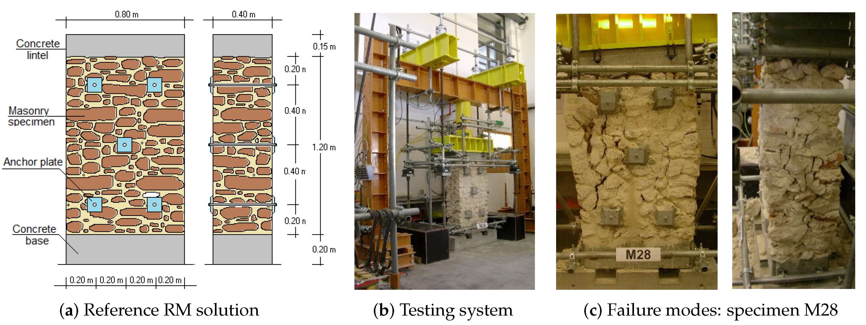
3. Experimental Campaign

An experimental campaign was conducted at NOVA FCT [2,6,10] on rubble stone masonry wall specimens built according to traditional Portuguese construction techniques and materials, considering transverse strengthening solutions. The objective of the experimental campaign was to quantify the increase in the mechanical strength relative to the unreinforced specimens (URM) and to assess the performances of various strengthening solutions. The URM specimens replicate the typical stone masonry found in ancient buildings that are representative of Portugal.

Overall, Pinho’s experimental work [2] involved the construction of 62 masonry specimens, including 42 “small specimens” with dimensions of $0.80\times 1.20\times 0.40$ m${}^3$ (length × height × thickness) used in uniaxial compression tests as URM reference specimens and subjected to different strengthening techniques. The remaining 20 specimens, referred to as “large specimens” with dimensions of $1.20\times 1.20\times 0.40$ m${}^3$, were used in shear-compression tests, including URM specimens and specimens strengthened using the same techniques as those used for the small specimens.

The rubble masonry specimens that are numerically evaluated are part of the small specimens which were constructed on top of reinforced concrete bases with a height of $0.20$ m. A 1:3 ratio of mortar and stone was adopted, i.e., about 25% of the volume of each specimen was filled with hydrated air lime laying mortar and the remaining 75% was filled with irregular limestone blocks.

The volumetric composition of the hydrated air lime mortar was 1:3 (hydrated air lime:sand) with a sand mixture consisting of equal parts of river sand and yellow pit sand. The water to hydrated air lime ratio was 1.2:1. The URM specimens were constructed in a manner that the two leaves were tied by through stones, which were placed $1/3$ and $2/3$ of the way up the specimens. To ensure uniform load distribution on the masonry, reinforced concrete beams (lintels) were constructed on top of the specimens.

The three specimens used in this study, M28, M41, and M44, were strengthened with transverse confinement systems consisting of independent steel transverse connectors of M12 galvanized steel-threaded rods tested under compression loads. The connectors were applied by drilling 16 mm diameter holes through the specimens. Each connector corresponds to a 12 mm diameter threaded–galvanized steel bar, tightened by nuts and steel plates measuring $100\times 100\times 5$ mm${}^3$ at both ends, using a torque wrench. The holes were blown through with a compressed air jet and then washed out and injected with a pozzolanic micro mortar (through PVC tubes applied for this purpose) using a manual pump under low pressure. Finally, the connectors were tightened by a dynamometric spanner with a torsional moment of 1 kg·m.

Figure 4 shows a schematic representation of the specimens strengthened by transverse steel connectors, the experimental testing system, and the frontal and lateral final failure of a specimen (M28) [2,6,10].

The transverse confinement system is arranged in “quincunxes” spaced $0.40$ m (corresponding to the thickness of the specimen) in both the horizontal and vertical directions as shown in Figure 4a.

Table 1. Experimental results obtained in axial compression (monotonic tests) on specimens strengthened by transverse confinement (M41, M44, and M28) and the URM specimens (M43, M21, and M32) [2,6].

Strengthening Solution	Specimens	Age(★) [Days]	${\mathit{F}}^{\mathit{max}}$  [kN]	${\mathit{\sigma }}^{\mathit{max}}$  [MPa]	${\mathit{\delta }}_{\mathit{v}}^{{\mathit{F}}_{\mathit{max}}}$  [mm]	${\mathit{\epsilon }}_{\mathit{v}}^{{\mathit{F}}_{\mathit{max}}}$  [${}^{\mathbf{o}}/{}_{\mathbf{oo}}$]	E [GPa]
Transverse steel connectors	M41	925	168.5	0.53	4.0	3.3	0.477
	M44	927	226.0	0.71	5.8	4.8	0.485
	M28	931	203.3	0.64	4.3	3.6	0.505
	RM Average	–	199.3	0.63	4.7	3.9	0.489
URM specimens	M43	618	134.2	0.42	6.8	5.7	0.239
	M21	626	127.7	0.40	6.4	5.3	0.409
	M32	638	148.5	0.46	4.3	3.6	0.267
	URM Average	–	136.8	0.43	5.8	4.9	0.305

${}^{(★)}$ Age at testing.

presents the results obtained in uniaxial compression tests for specimens M41, M44, and M28, as well as the results obtained for the reference URM specimens.

4. Numerical Modeling

Based on the experimental results, numerical modeling is carried out to assess the effect of the transverse steel connectors on the behavior of the strengthened rubble stone walls under simple compression loading using a 2D reinforced particle model.

4.1. 2D-PM Numerical Model Generation

The numerical models were defined from the lateral sides of the tested rubble masonry walls [2], which have a width of $0.40$ m. As demonstrated in [24], the use of the 2D-PM model of the lateral sides allows for the evaluation of peak strength and overall wall behavior with lower computational costs compared to the 2D-PM model of the frontal faces.

The generation of the 2D-PM model for the URM rubble masonry wall follows the same procedure as adopted in [24]. In the discretization of each stone element, with an average size of $16.7$ cm, a particle model with a uniform radius distribution ranging between $0.003$ mm to $0.005$ m was adopted. In the discretization of the mortar, a uniform radius distribution between $0.00714$ m and $0.00119$ m was adopted, where the maximum radius value corresponds to the maximum dimension of the sand used in the laying mortar [2].

For the RM models, the steel connectors, connector–stone, and connector–mortar interfaces also need to be defined. Each steel connector bar is discretized with 20 finite plane frame elements. The nodal points at the end of each connector are rigidly connected to the square rigid plates, $0.10$ m in length and $0.05$ m thick, which interact with the particles (mortar and stone) in direct contact.

Figure 5 presents the 2D-PM and 2D-PMR models developed from the lateral faces of the unreinforced (URM) [24] and reinforced (RM) rubble stone masonry walls. Note that the 2D-PMR models representing the one- and two-level strengthening scheme will later be used in the parametric analyses.

The scheme adopted with three levels of steel connectors corresponds to the reinforcement scheme used in the experimental tests, as shown in Figure 5d. In this model, the end connectors are represented by $2\times 12$ mm diameter steel connectors, while the connector at mid-height is represented by a single 12 mm diameter bar.

In the other strengthening solutions, with one- and two-level connectors, Figure 5b,c, each connector represents two bars with a diameter of 12 mm. The elastic and strength properties adopted for the steel connectors were obtained during the experimental work [6], $E\approx 200$ GPa and ${\sigma }_y\approx 590$ MPa.

Table 2. Number of particles and contacts for 2D-PM masonry models.

Model	Particles		Contacts
	Stone(s)	Mortar(m)	m–m	m–s	s–s
Lateral	7501	45,381	20,034	127,176	10,154

presents the number of particles adopted in the rubble stone masonry wall discretization, as well as the number of contacts present in the adopted 2D-PM model, according to the type of contact: stone/stone (s–s), mortar/stone (m–s), and mortar/mortar (m–m).

The adopted model corresponds to the lateral coarse model adopted in [24], which was shown to predict a response closer to that predicted by a more refined model, with a significant reduction in simulation times.

4.2. Contact Parameter Calibration

In [24], the elastic and strength contact properties of each type of contact were calibrated based on the experimental results presented in [2] and on some tests performed in the scope of the modeling work with PM-type models, namely uniaxial compression tests on stone and mortar. The s–s contact properties were calibrated on $0.20$ m × 0.20 m specimens and the m–m contact properties were calibrated on $0.04$ m × 0.04 m models. In [24], the calibration procedure is explained in more detail and, therefore, is not reproduced here. Figure 6 shows a typical final crack pattern obtained in uniaxial compression for the calibrated contact parameters representative of the mortar.

Table 3. Calibrated contact elastic and strength properties [24].

Contacts	$\overline{\mathit{E}}$  [GPa]	$\mathit{\alpha }$  [–]	${\mathit{\sigma }}_{\mathit{nt},\mathit{c}}$  [MPa]	${\mathit{\tau }}_{\mathit{c}}$  [MPa]	${\mathit{\mu }}_{\mathit{c}}$  [–]	${\mathit{G}}_{\mathit{f},\mathit{n}}$  [N/m]	${\mathit{G}}_{\mathit{f},\mathit{s}}$  [N/m]
s–s	8.60	0.11	8.90	35.7	1.0	0.3838	56.1403
m–m & m–s	0.09	0.43	0.16	0.16	1.0	0.0013	0.0030

presents the calibrated properties for each contact type, as shown, the properties of the m–m contact were adopted for the m–s contact.

In the normal direction under compression, a contact model with a yield plateau for a compression stress value of $0.80$ MPa was adopted, close to the maximum value in the simple compression of the laying mortar [2]. A yield plateau is required because, as shown in [24], high normal contact compression forces were found to occur at some mortar contacts, due to the heterogeneity present in the masonry walls.

Table 4. Experimental and numerical macroscopic values of the elastic and strength properties.

(a) Experimental values [2]
Material	$\mathit{E}$ [GPa]	$\nu$	${\sigma }_{\mathit{c}}$ [MPa]	${\sigma }_{\mathit{t}.\mathit{fl}}$ [MPa]
mortar	0.075	0.16	0.65	0.3
stone	6.0	0.3	47.8	–
(b) Numerical predictions after calibration [24]
Material	$\mathit{E}$ [GPa]	$\nu$	${\sigma }_{\mathit{c}}$ [MPa]	${\sigma }_{\mathit{t}.\mathit{fl}}$ [MPa]
mortar	0.075	0.16	0.66	0.16
stone	6.0	0.3	47.8	–

shows the elastic and strength contact properties of each component obtained numerically after calibration, as well as the known experimental values. For more details on the calibration process, see [24].

5. 2D-PM Reinforced Model Prediction

To validate the 2D-PMR modeling approach, the response of the three-level strengthening solution that follows the same reinforcing scheme adopted experimentally was simulated. In the experimental studies being modeled, the bond between the connectors and the masonry wall was not evaluated through pull-out tests. Due to the uncertainty regarding the stiffness and strength properties of the bar-particle interface, the numerical results of the RM reference model are presented for both the strong and weak bond approaches, as described in Section 2.4. Figure 7 presents the stress–displacement curves obtained experimentally in [2] for RM walls M21, M43, M44, and M28, as well as the results for the 2D-PM URM numerical model and the 2D-PMR models with the three-level strengthening solution that follows the same scheme adopted experimentally, considering both strong bond (2D-PM-L3-SB) and weak bond (2D-PM-L3-WB) approaches.

From the analysis of Figure 7, it can be observed that the numerical model without reinforcement (MP-2D), after a calibration procedure, is able to predict a stress–displacement curve with an evolution close to the curves obtained experimentally for walls M21 and M43 [2]. For more details related to the adopted numerical approach, see [24]. From Figure 7, it can be seen that the (2D-PM-L3-SB) and (2D-PM-L3-WB) models, compared to the numerical model without reinforcement, lead to an increase in the peak force and predicted ductility.

The predicted numerical results using the 2D-PMR model show that the reinforcement solution with 3 levels of reinforcement, as adopted in the experimental tests, leads to an increase in the peak stress values between 20% (for weak particle/bar bond) and 50% (for high particle/bar bond). These predicted values fall within the range of the values obtained experimentally, where an average increase in strength of 47% was observed for the walls with connectors compared to the reference URM walls.

Table 5. Experimental and numerical values of the peak stress.

Model		${\mathit{\sigma }}_{\mathit{v}}^{\mathit{max}}$ [MPa]
Numerical	MP-2D	0.50
	2D-PM-L3-SB	0.75
	2D-PM-L3-WB	0.60
Experimental	Average URM [2] ${}^{★}$	0.43
	Average RM [2] ${}^{\#}$	0.63

${}^{★}$ URM average values: specimens M43, M21, and M32 [2]; ${}^{\#}$ RM average values: specimens M41, M44, and M28 [2].

presents the peak stress values obtained numerically and the average of the experimental values.

The increase obtained experimentally is slightly higher than the value obtained numerically for a weak bond assumption. This can be explained by the effect of carbonation (among other factors, such as the heterogeneity of the masonry and the position of the connectors relative to the stones placed on the face of the walls, e.g., crossing the stones or crossing the joints) since the walls tested with the reinforcement solution are older than the walls tested experimentally without reinforcement. As shown, the developed 2D-PM reinforced models predict values within the order of magnitude of the experimentally obtained values.

The damage evolution throughout the uniaxial compression test for the 2D-PM and 2D-PMR numerical models is shown in Figure 8.

Cracking occurs in all 2D-PMR models for a uniaxial load of around $0.40$ MPa. In the unreinforced 2D-PM model, there is a steep increase in tensile cracks, whereas in the 2D-PMR strengthened numerical models, both adopting weak and strong bonds, the increase in tensile cracks is much more controlled as the steel bars restrain their growth. In both strengthened 2D-PMR models, there is a significant increase in cracked contacts that occurred under tensile or shear and are found under compression due to the lateral restraint imposed by the steel connectors.

Figure 9 presents the distribution of contact damage obtained for the maximum displacement value for both the URM 2D-PM and the tested 2D-PMR models. As shown, in comparison to the model without reinforcement, in both reinforced models, the damage at the contacts in the area of influence of the connectors and the crack opening is practically non-existent, as the connectors are able to restrict the propagation of damage, thus preventing the lateral detachment of stones.

In the strengthened models, the overall deformability at the maximum displacement value, the upper plate rotation, and the crack opening are much lower. In the experimental tests [2,6], an improvement in the failure conditions of the walls reinforced with steel elements was observed. The strengthened walls, when compared with the unreinforced walls, showed higher masonry integrity and cohesion.

The evolution of the axial stress at the steel connectors’ mid-span at each location ($a_1-a_3$), is presented in Figure 10 for both strengthening 2D-PMR models. As shown, the largest difference between the numerical model with a strong (SB) and weak (WB) bond occurs in the steel connector at mid-height and in the upper connector, with the difference being more pronounced in the connector at mid-height. This is associated with the final failure mode observed in the strengthened models, which is due to the rotation of the part of the wall above the upper connector. Figure 10 also shows that a stress level close to the yield value (approximately 590 MPa) is reached only at the mid-level connectors since only a single steel connector is placed at this height.

6. Parametric Studies

Overall, the presented numerical studies demonstrate that the predictions of the 2D-PMR-reinforced model are in good agreement with experimental results [2], particularly in terms of the corresponding failure modes and the increase in the maximum uniaxial compression value and ductility. Subsequently, several parametric studies are presented, which demonstrate the potential of the 2D-PMR models in the development of such reinforcement solutions, including the definition of bar characteristics, positioning, quantification, and the relevance of the importance of grout injection in the drilled holes.

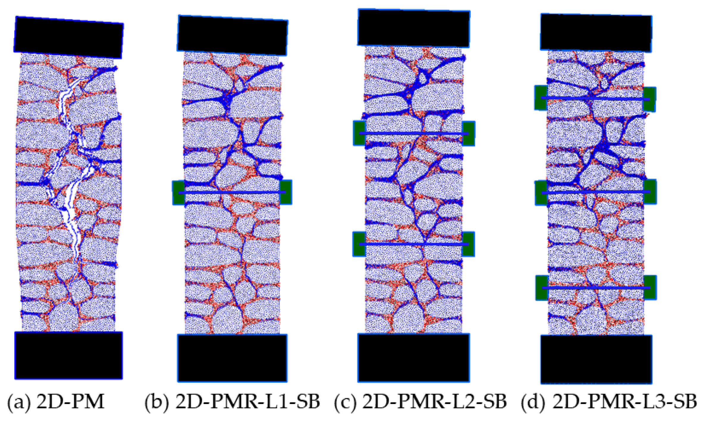
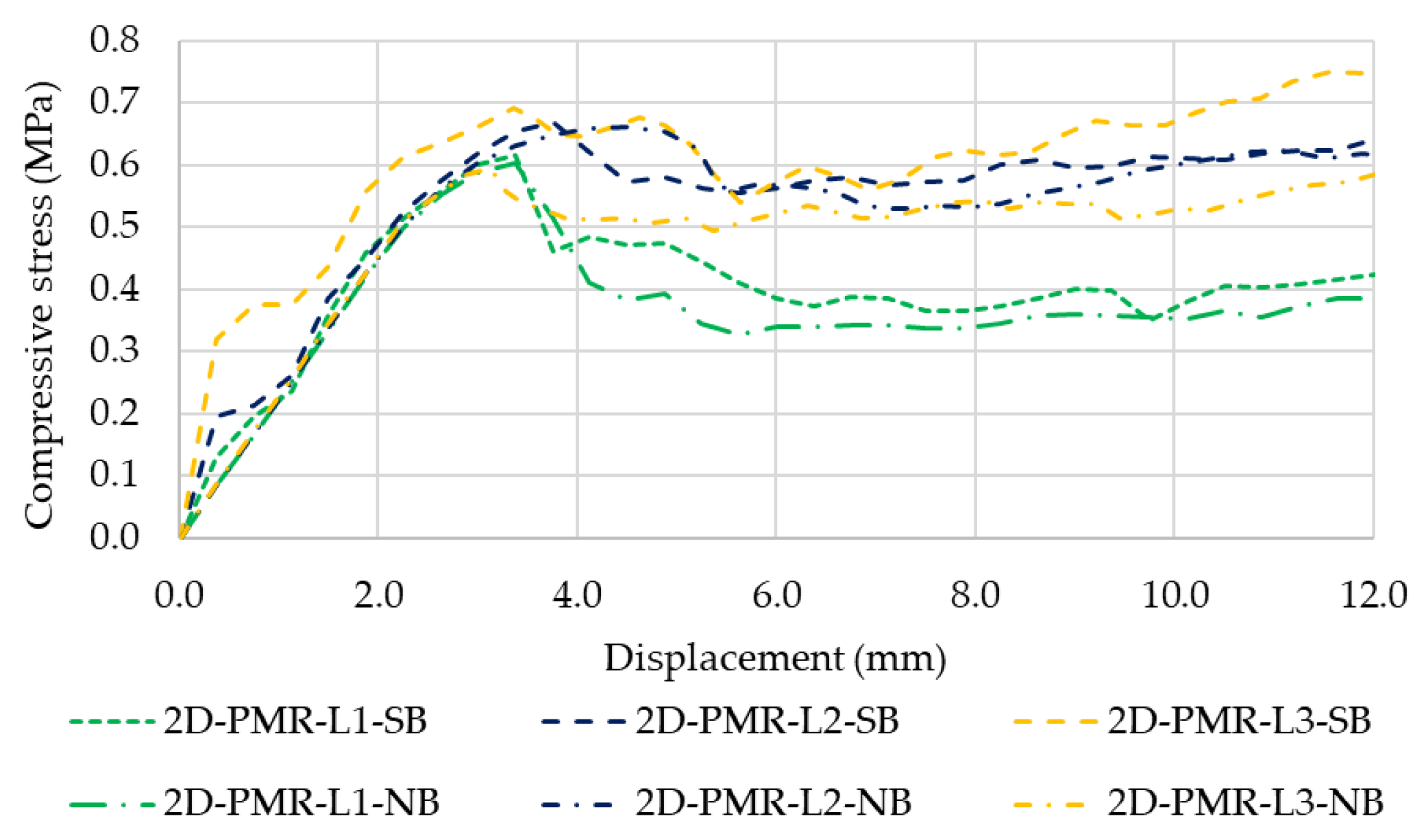
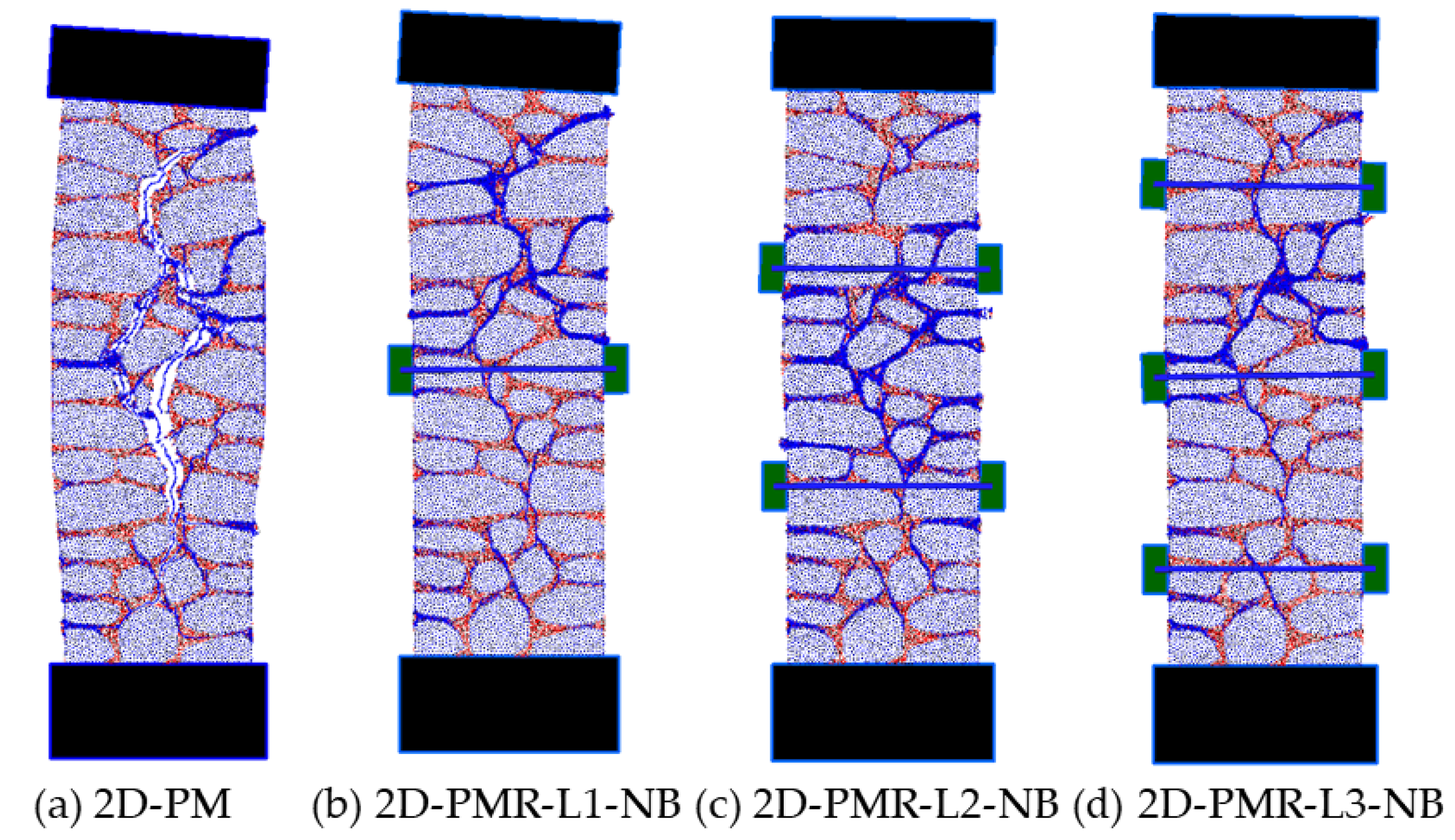
6.1. Reinforcement Scheme

In the experimental work, only one steel connector-based strengthening solution, namely the three levels of steel connectors (2D-PM-L3), was tested. Taking the numerical results of the 2D-PM-L3 solution as a reference, two other strengthening solutions were numerically assessed, i.e., with only one level of reinforcement at mid-height (2D-PM-L1) and with two levels of reinforcement at a quarter of the height (2D-PM-L2), as shown in Figure 5b,c.

Figure 11 presents the stress–displacement curves obtained for the 2D-PMR numerical models for the three strengthening schemes (-L1, -L2, -L3), considering the strong bond (SB) and the weak bond (WB) approach, as well as the results obtained for the 2D-PM model of the URM.

As shown in Figure 11, the two-level (-L2) strengthening scheme predicts a response similar to the response obtained with the strengthening scheme adopted in the experimental work (-L3) for both bond options. The two-level scheme with a weak bond approach predicts a higher peak stress response than that predicted with a three-level scheme.

When the strong bond approach is adopted, the predicted increase in the peak value varies between 23% for one-level (L1) and 50% for three-level (L3). In the weak bond approach, the predicted increase in the peak value varies between 21% for one-level (L1) and 33% for two-level (L2). In the weak bond approach, the increase in peak strength is less noticeable with a three-level (L3) solution (20% increase). These results are summarized in

Table 6. Peak strength increase compared with the unreinforced wall 2D-PMR model.

Bond Type	Model	$\Delta {\mathit{\sigma }}_{\mathit{v}}^{\mathit{max}}[\%]$
Strong Bond	2D-PM-L1-SB	23
	2D-PM-L2-SB	38
	2D-PM-L3-SB	50
Weak Bond	2D-PM-L1-WB	21
	2D-PM-L2-WB	33
	2D-PM-L3-WB	20

.

In Figure 12, the evolution of axial stress at the steel connectors’ mid-span is presented for the several MP-2DR models at each connector location ($a_1-a_3$). It shows that a similar response is obtained with both weak and strong bond approaches. Figure 12 also shows that the axial stress at the bars is far from the yield value for both L1 and L2 of reinforcement.

Figure 13 presents the contact damage distribution obtained at the maximum displacement value for the various tested 2D-PMR models, for different reinforcement levels, adopting a strong bond approach. A similar behavior was observed when adopting a weak bond approach. As shown, compared to the 2D-PM response of the URM, in the MP-2DR models, as the number of reinforcement levels is increased: (i) the deformability of the numerical model at the maximum displacement value decreases; (ii) the rotation of the upper plate decreases; and (iii) the observed crack opening decreases.

The numerical results presented demonstrate that a single layer of steel bars at mid-height (L1) provides a similar increase in ductility and peak strength for both the strong bond (23%) and weak bond approaches (21%). When using a weak bond approach, the two-level solution (L2) predicts a higher peak strength increase (30%) compared to the peak strength increase predicted with a three-level reinforcement solution (20%). In a strong bond approach, the two-level solution predicts a peak strength increase (38%), which is slightly lower than the peak strength increase predicted with a three-level reinforcement solution (50%).

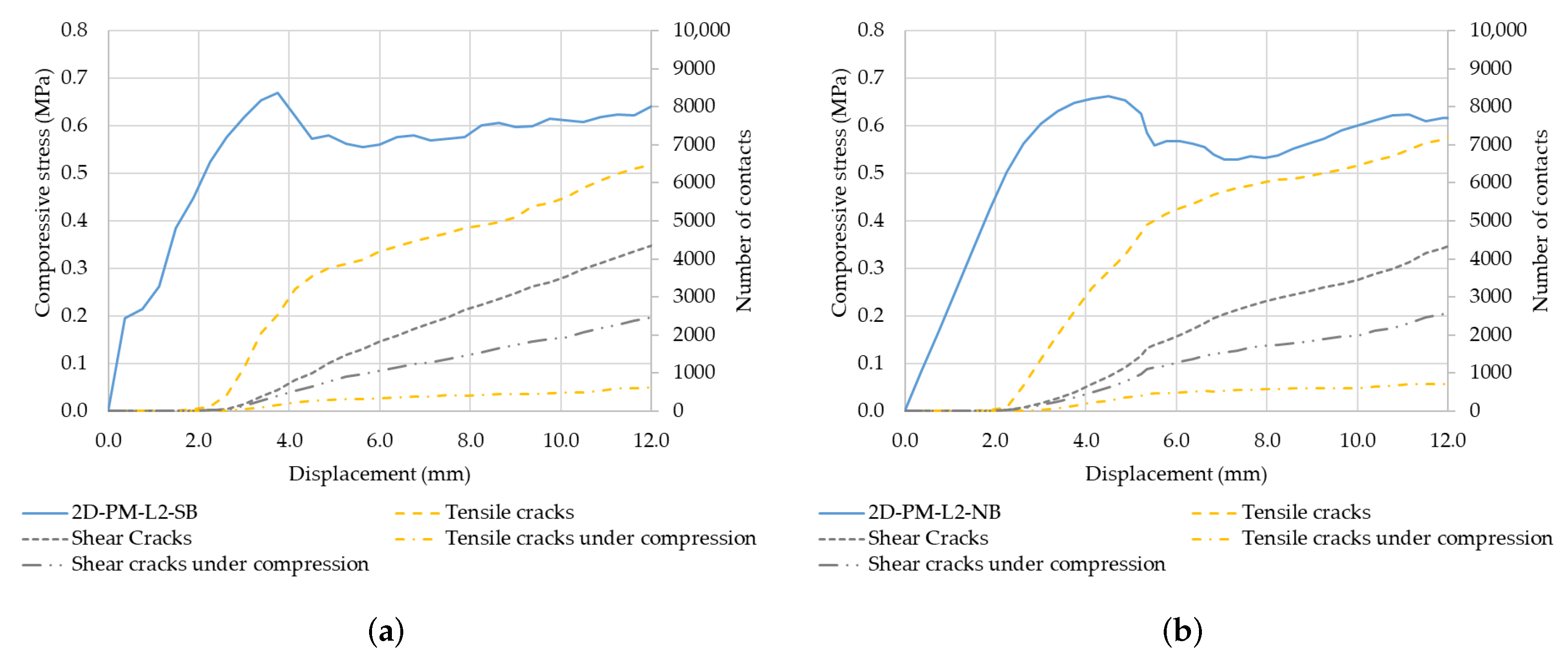
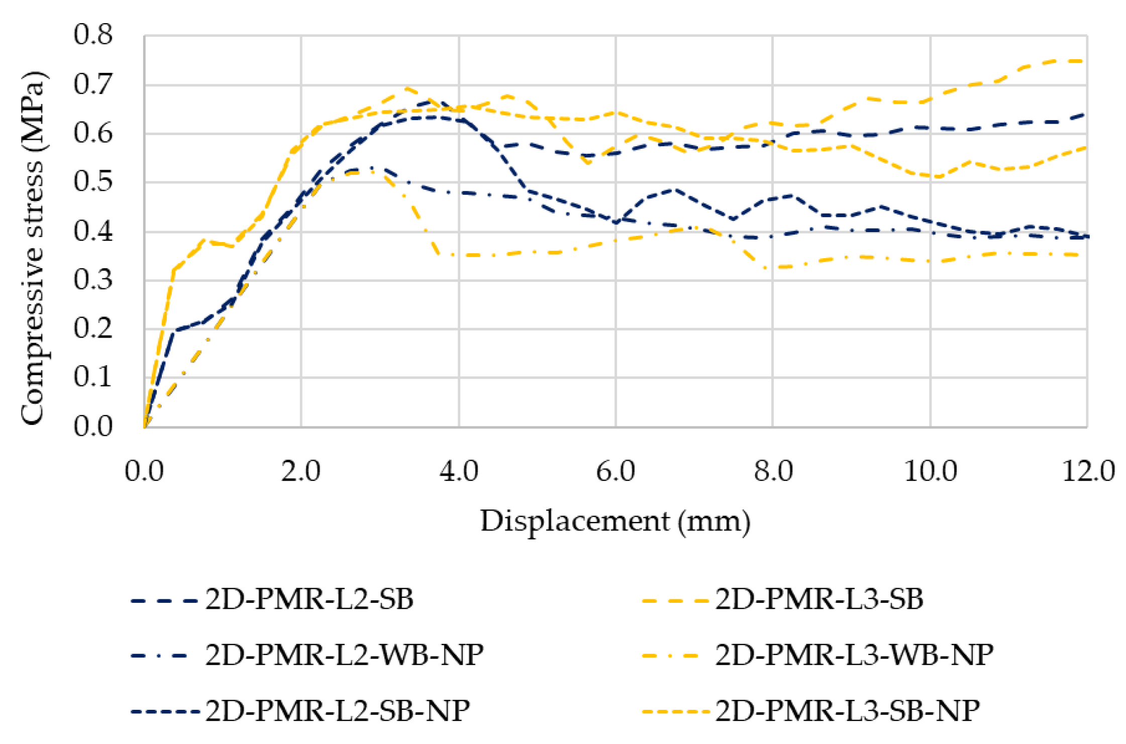
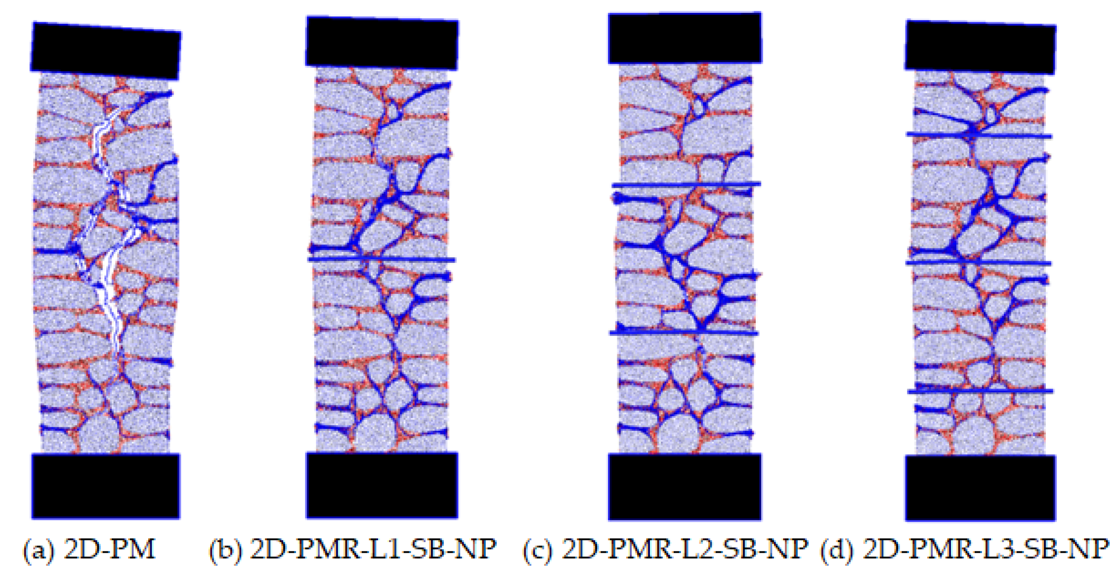
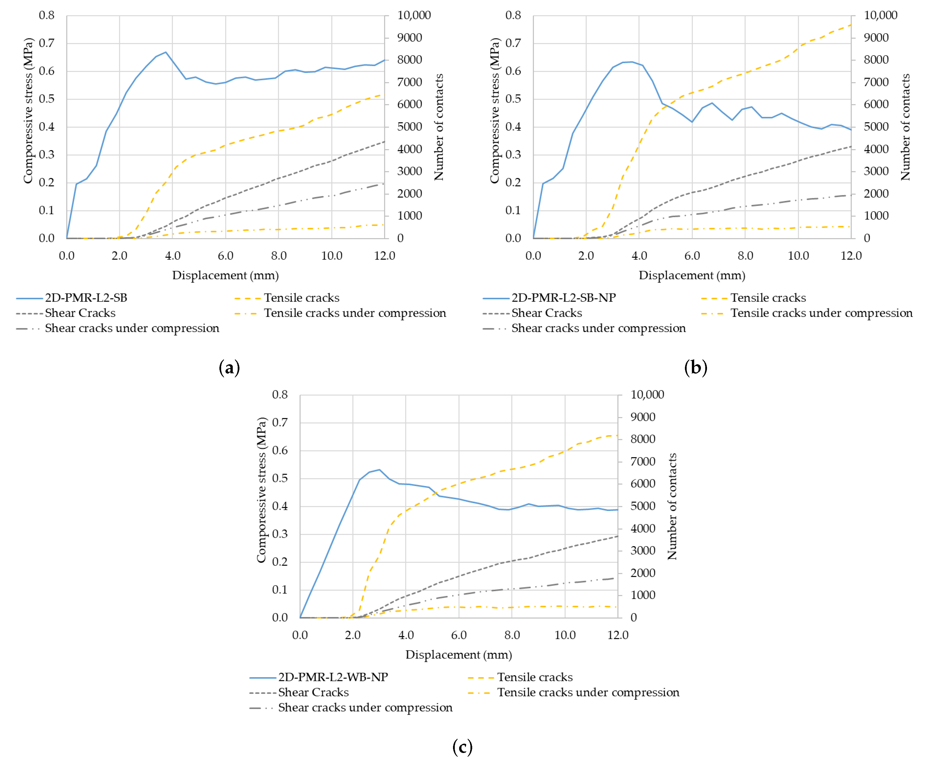
6.2. Connector–Particle Bond

In the experimental work, steel connectors with a diameter of 12 mm were placed in 16 mm holes drilled in the walls, which were subsequently filled with mortar to ensure a bond between the wall components and the steel connectors. As shown in the previous numerical analysis, similar results are obtained with strong and weak bond assumptions.

In this section, we evaluate the possibility of having no bond between the steel connector and the wall component, which was not tested experimentally. Compared with the adopted experimental procedure, this solution reduces the strengthening procedure requirements, namely drilling a higher diameter hole and injecting it with a pozzolanic micro mortar.

The stress–displacement curves obtained for the 2D-PMR numerical models, considering a strong bond (SB) and no bond (NB), are presented in Figure 14.

From the results presented in Figure 14, it can be seen that a strong bond assumption always leads to a higher peak and a more ductile response, but the response predicted with the 2D-PMR model without a bond is very similar to that predicted with a strong bond. This indicates that the confinement provided by the plate connected to the steel bars applies to the rubble masonry walls and is sufficient enough to guarantee the required behavior improvement under uniaxial compression.

Figure 15 shows the damage evolution throughout the uniaxial compression test for the 2D-PMR numerical models with a strong bond and without a bond for a two-level reinforcement scheme.

The cracking evolution is similar under both bond assumptions in the 2D-PMR model. However, in the model without a bond, a higher number of tensile cracks are observed compared to the strong bond assumption. The evolution of shear cracks and the evolution of cracked contacts that occurred under tensile or shear and are found under compression due to the lateral restraint imposed by the steel connectors are very similar under both bond assumptions. This shows that the confinement produced by the plates connected to the steel bars is sufficient to ensure similar strengthening.

Figure 16 presents the axial stress evolution at the mid-span of the steel connectors for the two-level strengthening scheme, MP-2DR models, for both the strong bond and no-bond cases. Similar results were found for the one-level and three-level strengthening schemes. As shown, the MP-2DR models predict a similar response without a bond as with a strong bond approach. Notably, in the 2D-PMR model with a two-level scheme without a bond, the axial stress evolution at both levels is more symmetric than with a strong bond approach.

The contact damage distribution obtained at the maximum displacement value for the 2D-PM and for the various tested 2D-PMR models, for different reinforcement levels, adopting a no-bond approach, is presented in Figure 17. The predicted damage patterns are similar to those predicted with a 2D-PMR model with a strong bond approach.

The presented numerical results need to be validated by experimental testing, but they clearly indicate that when plates are adopted, the bond between the connectors and the wall components is not relevant and, therefore, more economical strengthening solutions can be adopted.

6.3. Lateral Plate Influence

In the experimental work, the steel connectors were connected to $0.10$ m square lateral plates measuring $0.05$ m in thickness, with the interposition of a cement mortar and sand layer (1:3) between the plate and the masonry. However, on site, it may not be feasible to apply the square plates in one or both wall faces. The developed 2D-PM reinforced model was adopted to assess the relevance of the square plates in the lateral confinement effect and the overall behavior.

In Figure 18, the stress–displacement curves obtained for the 2D-PM reinforced numerical models, with a strong bond (SB) and lateral plate, with a weak bond (WB) without the lateral plate (NP), and with a strong bond (SB) without the lateral plate (NP) for two-level and three-level strengthening schemes are presented.

As shown in Figure 18, a weak bond assumption without a lateral plate only leads to a 5% increase in the peak strength, when compared with the value predicted with a 2D-PM URM model. Under a strong bond assumption, a significant increase in the peak strength and ductility can be obtained even if a lateral plate is not adopted.

Figure 19 presents the contact damage distribution obtained at the maximum displacement value for the 2D-PM URM model and the 2D-PMR models with a strong bond approach without a lateral plate for different reinforcement levels.

The overall predicted damage patterns without the plates are similar to those predicted with a 2D-PMR model with a strong bond approach and lateral plates, as seen in Figure 13; however, the contact damage is more distributed throughout the masonry wall when no plates are adopted. The confinement provided by the lateral plates reduces the damage occurrence in their vicinity, as observed in Figure 13.

Figure 20 shows the damage evolution throughout the uniaxial compression test for the 2D-PMR numerical models with a strong bond and plate, and for the 2D-PMR models without plates under strong and weak bond assumptions, for a two-level reinforcement scheme. In the 2D-PMR models without plates, regardless of the bond assumption, a higher number of tensile cracks occurs when compared to the strong bond with plate model.

The total number of cracks that occur under tensile or shear and are found under compression is much lower in the 2D-PMR model with plates, indicating that the confinement provided by the plates connected to the steel bars is crucial for effective strengthening. The presented numerical results clearly demonstrate the importance of the lateral plate in the strengthening mechanism. If a lateral plate cannot be adopted, the connector/wall bond becomes crucial for the strengthening mechanism to be effective.

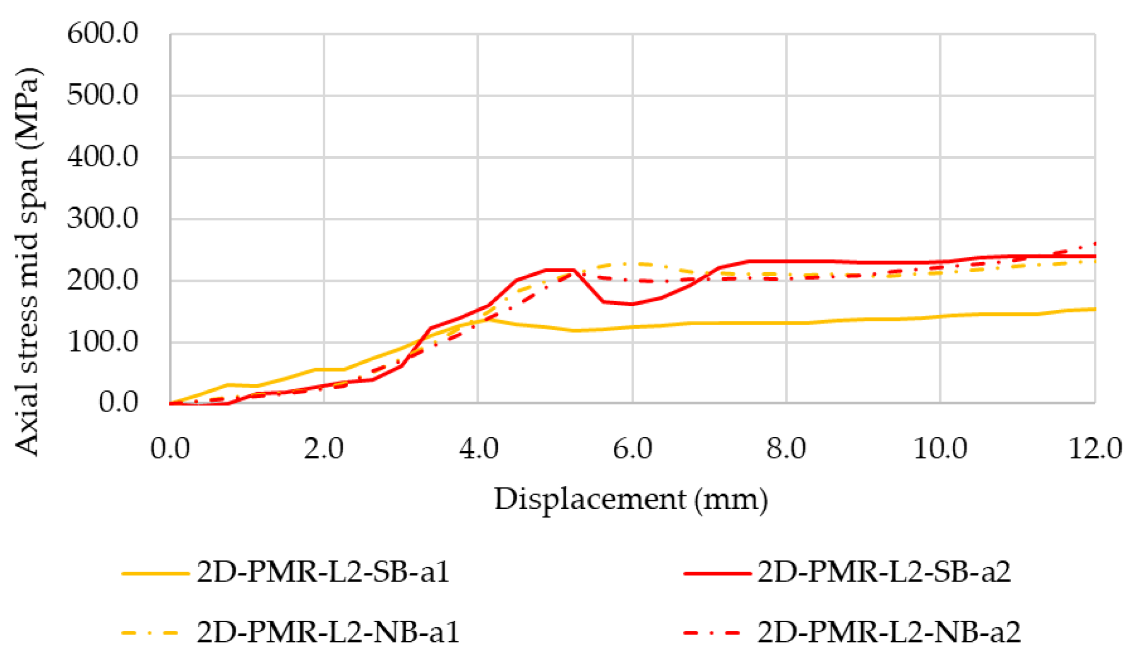
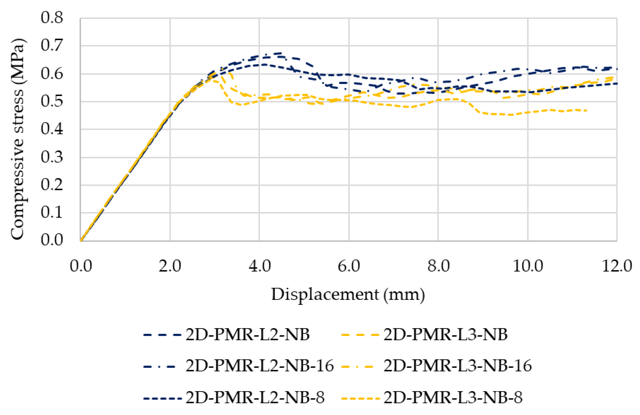
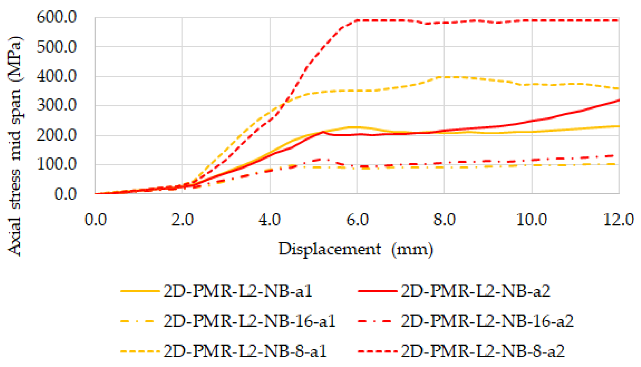
6.4. Steel Bar Diameter

In the experimental tests, it was not possible to evaluate the influence of the steel connector diameters in the strengthening mechanism; only steel connectors with 12 mm diameters were used. For this reason, several numerical analyses were carried out to evaluate the relevance of steel connector diameters, which have an influence on bar stiffness and strength. The 2D-PMR models with 8 mm and 16 mm diameter bars are evaluated under the no-bond assumption between the steel connectors and the wall components.

Figure 21 presents the stress–displacement curves obtained for the 2D-PMR numerical models with a three-level reinforcement solution without a bond and considering different connector diameters: 12 mm diameter (2D-PM-L3-NB), 16 mm diameter (2D-PM-L3-NB-16), and 8 mm diameter (2D-PM-L3-NB-8). As shown, the diameter range that is numerically assessed has little influence on the predicted response. As expected, the highest peak strength and ductility under uniaxial compression were predicted with the MP-2DR model with the largest diameter, but the overall response obtained with the smallest diameter is very similar.

Figure 22 presents the evolution of axial stress at the mid-span of steel connectors for MP-2DR models with a two-level strengthening scheme and a no-bond assumption for several tested connector diameters. As expected, the axial stress increases as the bar diameter decreases, and in the MP-2D-L2-NB-8 model, the steel connectors at the upper level reach the yielding stress value of 590 MPa. The axial stress evolution is very similar in all MP-2DR models until a vertical stress of $0.40$ MPa, where noticeable damage begins to occur in the particle assembly.

The presented numerical results indicate that an 8 mm steel connector diameter with elastic and strength properties (similar to that adopted in the experimental test) would have been sufficient to guarantee a similar strengthening effect.

7. Conclusions

Particle models (2D-PM) have shown their capability to predict complex macroscopic failure with simple interaction constitutive laws and have been successful in modeling the response of URM stone masonry walls in terms of maximum force, ductility, and the process of crack formation and propagation under uniaxial compressive loading conditions [24]. However, it should be noted that the contact parameters of each wall element, including mortar and stones, need to be calibrated beforehand using known standard experimental data [24].

In this work, we extend the PM modeling strategy proposed in [24] to investigate and assess the response of steel-based reinforced systems for existing two-leaf stone masonry walls subjected to axial compressive loading. We develop a 2D-PM reinforced model in which the steel connectors are discretized using FEM-based frame elements, and the stone–steel and mortar–steel interactions, through grouting, are modeled by a particle-bar contact interface. The proposed numerical scheme enables the 2D-PMR model to simulate the steel-based transverse confinement effect on rubble masonry walls.

To validate the proposed 2D-PMR model, a numerical evaluation was conducted on a steel connector reinforced system with a three-level reinforcement arrangement identical to the experimental specimens. The study concluded that the numerical results closely match the experimental results in terms of strength and ductility, the crack growth process, and the reduction in horizontal detachments. The 2D-PMR model was used to conduct parametric studies on the masonry specimen by varying the level of strengthening and the diameter of the steel bars to assess the influence of the bar-bond effect and lateral plates. Based on the results and the presented discussion, the following main conclusions can be drawn:

• The proposed 2D reinforced particle model formulation allows the 2D-PMR model to replicate the transverse confinement effect of steel-based reinforcement on rubble stone masonry walls. The formulation is straightforward and can be easily incorporated into similar models that use other commercial or open-source implementations.
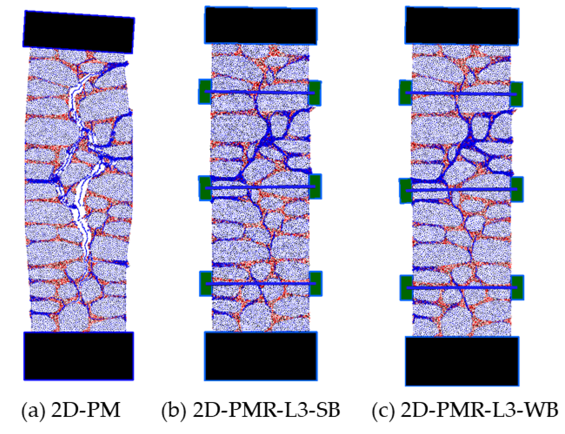
• The 2D-PMR model can predict the improved strength and ductility, the crack growth process, and the reduction in horizontal detachments of the masonry observed in the experimental tests of strengthened rubble stone masonry walls. Numerical results indicate that a strong particle/bar bond approach (50%) predicts a higher peak strength increase than the average increase in strength (47%) observed experimentally for the reference specimen.
• The presented discussion, from a numerical modeling perspective, regarding the relevance of the bond between the steel bar connectors, the presence and importance of the end plates, and the connectors’ diameters, provides useful information for the consolidation and understanding of this reinforcing technique.
• The results and discussions presented underline the complexity of capturing the accurate behavior of the existing/real rubble stone masonry walls and the difficulty in numerically estimating the effect of this intervention technique.
• Overall, the proposed 2D-PMR model can be adopted in the design phase of reinforcement solutions involving simple transverse confinement, particularly in the definition of bar characteristics, positioning, quantification, and in the assessment of the relevance of the grout injection in the application process of the steel connectors.

The performance of the proposed 2D-PMR model is encouraging and, therefore, further work is underway that will allow the 2D-PMR model to numerically evaluate other reinforcement techniques, namely, reinforced micro-concrete layers and textile reinforced mortar. The development of a 3D-PMR model is also being carried out. Given the computational restrictions, several modeling simplifications are being devised to keep the associated computational costs to a minimum.

References

1. National Institute of Statistic. Census 2011. Definitive Results; INE: Lisbon, Portugal, 2012; ISBN 978-989-25-0181-9. (In Portuguese) [Google Scholar]
2. Pinho, F.F.S. Ordinary Masonry Walls—Experimental Study with Unstrengthened and Strengthened Specimens. Ph.D. Thesis, Faculdade de Ciências e Tecnologia, Universidade Nova de Lisboa, Lisbon, Portugal, 2007. (In Portuguese). [Google Scholar]
3. Pinho, F.F.S.; Lúcio, V.J.G.; Baião, M.F.C. Rubble stone masonry walls in Portugal strengthened with reinforced micro-concrete layers. Bull. Earthq. Eng. 2012, 10, 161–180. [Google Scholar] [CrossRef]
4. Pinho, F.F.S.; Lúcio, V.J.G.; Baião, M.F.C. Rubble Stone Masonry Walls Strengthened by Three-Dimensional Steel Ties and Textile Reinforced Mortar Render, Under Compression. Int. J. Archit. Herit. 2014, 8, 670–689. [Google Scholar] [CrossRef]
5. Pinho, F.F.S.; Lúcio, V.J.G.; Baião, M.F.C. Rubble Stone Masonry Walls Strengthened by Three-Dimensional Steel Ties and Textile-Reinforced Mortar Render, Under Compression and Shear Loads. Int. J. Archit. Herit. 2015, 9, 844–858. [Google Scholar] [CrossRef]
6. Pinho, F.F.S.; Lúcio, V.J.G.; Baião, M.F.C. Experimental analysis of rubble stone masonry walls strengthened by transverse confinement under compression and compression-shear loadings. Int. J. Archit. Herit. 2018, 12, 91–113. [Google Scholar] [CrossRef]
7. Gkournelos, P.; Triantafillou, T.; Bournas, D. Seismic upgrading of existing masonry structures: A state-of-the-art review. Soil Dyn. Earthq. Eng. 2022, 161, 107428. [Google Scholar] [CrossRef]
8. Valluzzi, M.; Da Porto, F.; Modena, C. Behaviour of multi-leaf stone masonry walls strengthened by different intervention techniques. In Historical Constructions 2001; Universidade do Minho: Braga, Portugal, 2001; pp. 1023–1032. ISBN 972-8692-01-3. [Google Scholar]
9. Pinho, F.F.S. Structural Rehabilitation of Traditional Stone Masonry Walls; Science, Engineering and Technology Collection, Nova.FCT Editorial: Lisbon, Portugal, 2021; ISBN 978-989-54493-5-4. (In Portuguese) [Google Scholar]
10. Pinho, F.F.S.; Lúcio, V.J.G. Rubble Stone Masonry Walls in Portugal: Material Properties, Carbonation Depth and Mechanical Characterization. Int. J. Archit. Herit. 2017, 11, 685–702. [Google Scholar]
11. Corradi, M.; Borri, A.; Poverello, E.; Castori, G. The use of transverse connectors as reinforcement of multi-leaf walls. Mater. Struct. 2016, 50, 114. [Google Scholar] [CrossRef] [Green Version]
12. Rots, J.G. Numerical simulation of cracking in structural masonry. Heron 1991, 36, 49–63. [Google Scholar]
13. Lourenço, P.B. Computations on historic masonry structures. Prog. Struct. Eng. Mater. 2002, 4, 301–319. [Google Scholar] [CrossRef]
14. Lourenço, P.B.; Rots, J.G. Multisurface Interface Model for Analysis of Masonry Structures. J. Eng. Mech. 1997, 123, 660–668. [Google Scholar] [CrossRef]
15. Lemos, J. Discrete element modelling of the seismic behaviour of stone masonry arches. In Computer Methods in Structural Masonry—4 Fourth International Symposium, 1st ed.; Pande, G., Middleton, J., Kralj, B., Eds.; CRC Press: London, UK, 1998; pp. 220–227. ISBN 9780419235408. [Google Scholar]
16. Sarhosis, V.; Lemos, J. A detailed micro-modelling approach for the structural analysis of masonry assemblages. Comput. Struct. 2018, 206, 66–81. [Google Scholar] [CrossRef]
17. Azevedo, N.M.; Lemos, J.V.; Rocha, J.d.A. Discrete Element Particle Modelling of Stone Masonry. In Computational Modeling of Masonry Structures Using the Discrete Element Method; IGI Global: Hershey, PA, USA, 2016; pp. 146–170. [Google Scholar] [CrossRef]
18. Smoljanović, H.; Živaljić, N.; Željana, N. A combined finite-discrete element analysis of dry stone masonry structures. Eng. Struct. 2013, 52, 89–100. [Google Scholar] [CrossRef]
19. Azevedo, N.M.; Lemos, J.V. A Hybrid Particle/Finite Element Model with Surface Roughness for Stone Masonry Analysis. Appl. Mech. 2022, 3, 608–627. [Google Scholar] [CrossRef]
20. Thavalingam, A.; Bicanic, N.; Robinson, J.I.; Ponniah, D.A. Computational framework for discontinuous modelling of masonry arch bridges. Comput. Struct. 2001, 79, 1821–1830. [Google Scholar] [CrossRef]
21. Azevedo, N.M.; Lemos, J.; Rocha, J.d. Influence of aggregate deformation and contact behaviour on discrete particle modelling of fracture of concrete. Eng. Fract. Mech. 2008, 75, 1569–1586. [Google Scholar] [CrossRef]
22. Azevedo, N.M.; Candeias, M.; Gouveia, F. A Rigid Particle Model for Rock Fracture Following the Voronoi Tessellation of the Grain Structure: Formulation and Validation. Rock Mech. Rock Eng. 2014, 48, 535–557. [Google Scholar] [CrossRef]
23. Chen, X.; Wang, X.; Wang, H.; Agrawal, A.K.; Chan, A.H.; Cheng, Y. Simulating the failure of masonry walls subjected to support settlement with the combined finite-discrete element method. J. Build. Eng. 2021, 43, 102558. [Google Scholar] [CrossRef]
24. Azevedo, N.M.; Pinho, F.F.S.; Cismaşiu, I.; Souza, M. Prediction of Rubble-Stone Masonry Walls Response under Axial Compression Using 2D Particle Modelling. Buildings 2022, 12, 1283. [Google Scholar] [CrossRef]
25. Azevedo, N.M. A Rigid Particle Discrete Element Model for the Fracture Analysis of Plain and Reinforced Concrete. Ph.D. Thesis, Herito-Watt University, Edinburgh, UK, 2003. [Google Scholar]
26. Senthivel, R.; Lourenço, P.B. Finite element modelling of deformation characteristics of historical stone masonry shear walls. Eng. Struct. 2009, 31, 1930–1943. [Google Scholar] [CrossRef] [Green Version]
27. Azevedo, N.M.; Pinho, F.F.S.; Cismasiu, I.; Souza, M.B.d. Modeling traditional stone masonry walls with a particle model. In Proceedings of the Congresso Nacional Reabilitar & Betão Estrutural 2020, LNEC, Lisbon, Portugal, 3–5 November 2021; p. 10. (In Portuguese). [Google Scholar]
28. CEB-FIP MODEL CODE 1990; Thomas Telford Publishing: London, UK, 1993. [CrossRef]
Figure 1. Bilinear softening contact model under tensile loading and shear and the yielding contact model under compressive loading. (a) Normal direction; (b) Shear direction.
Buildings 13 00987 g001
Figure 2. Stone masonry wall 2D-PM model generation procedure. (a) Masonry wall; (b) Stone unit particle assembly; (c) Mortar particle assembly.
Buildings 13 00987 g002
Figure 3. Steel bar-particle contact interface geometry.
Buildings 13 00987 g003
Figure 4. Setup for compression tests of the RM wall specimens and final failure modes [6]. (a) Schematic representation of the reinforcement solution with steel connectors (Specimens M41, M44, and M28); (b) axial compression testing system; and (c) frontal and lateral views of the failure mode of specimen M28. See [2,6] for more details.
Buildings 13 00987 g004
Figure 5. The 2D-PM and 2D-PMR models of the lateral faces of the rubble masonry walls with and without connectors; (a) without reinforcement; (b) one-level, (c) two-level, and (d) three-level, as in the experimental test.
Buildings 13 00987 g005
Figure 6. The 2D-PM model calibration: final crack pattern for the uniaxial compression test of the mortar model.
Buildings 13 00987 g006
Figure 7. Results of the URM and the reference reinforced (three-level) 2D-PMR models; stress–displacement curves in comparison with the experimental results [2].
Buildings 13 00987 g007
Figure 8. Results of the URM and reference RM 2D-PMR models: stress–displacement diagram and crack evolution. (a) Without confinement; (b) Three levels–strong bond; (c) Three levels–weak bond.
Buildings 13 00987 g008
Figure 9. Numerical models: contact damage distribution (a) without and (b,c) with reinforcement (strong and weak bonds).
Buildings 13 00987 g009
Figure 10. Numerical models 2D-PM-L3-SB and 2D-PM-L3-WB: axial stress at the steel connectors ( a 1 a 2 a 3 ), mid-span versus the plate vertical displacement diagram.
Buildings 13 00987 g010
Figure 11. Numerical models: stress–displacement diagrams for the URM 2D-PM model and the 2D-PMR model for various reinforcement levels. (a) Strong bond; (b) Weak bond.
Buildings 13 00987 g011
Figure 12. Axial stress at the steel connectors mid-span versus the plate’s vertical displacement diagram: 2D-PMR models for various reinforcement levels and bond strength. (a) Strong bond; (b) Weak bond.
Buildings 13 00987 g012
Figure 13. Numerical models: contact damage distribution with and without various reinforcement levels and a strong bond.
Buildings 13 00987 g013
Figure 14. Stress–displacement diagrams for the 2D-PMR models: strong bond versus no bond.
Buildings 13 00987 g014
Figure 15. Stress–displacement diagram and crack evolution for 2D-PMR models with (a) strong bond approach and (b) without a bond.
Buildings 13 00987 g015
Figure 16. Axial stress at the steel connectors mid-span versus the plate’s vertical displacement diagram for the 2D-PMR models of the two-level strengthening scheme: bond influence.
Buildings 13 00987 g016
Figure 17. Numerical models: contact damage distribution for URM and RM models without a bond.
Buildings 13 00987 g017
Figure 18. Stress–displacement diagrams for the 2D-PMR L2 and L3 models: strong and weak bond assumptions without lateral plates and a strong bond with lateral plates.
Buildings 13 00987 g018
Figure 19. Contact damage distribution of the numerical models: URM and RM models with a strong bond without a lateral plate.
Buildings 13 00987 g019
Figure 20. Stress–displacement diagram and crack evolution for the 2D-PMR models with and without plates for strong and weak bond approaches. (a) 2D-PM-L2-SB; (b) 2D-PM-L2-SB-NP; (c) 2D-PM-L2-WB-NP.
Buildings 13 00987 g020
Figure 21. Stress–displacement diagrams for 2D-PMR models with a three-level reinforcement solution and a no-bond assumption: connector diameter assessment.
Buildings 13 00987 g021
Figure 22. Axial stress at the steel connectors’ mid-span versus the plate vertical displacement diagram for 2D-PMR models with two levels of reinforcement without a bond assumption: connector diameter assessment.
Buildings 13 00987 g022