Long-Term Impacts of Temperature Gradients on a Concrete-Encased Steel I-Girder Experiment—Field-Monitored Data

Abstract

This article delves into an investigation of an experimental steel I-girder section encased in concrete and its instrumentation for the purpose of analyzing temperature distributions in concrete bridges. The study aims to examine the effect of differing air temperatures and thermal loads resulting from solar radiation. Structural health monitoring sensors, including a range of temperature sensors, were connected with the girder to monitor the structural performance using the data acquisition system constantly. The collection of experimental data took place during an exceptionally cold season, and the results of the study revealed both the lateral and vertical distribution of thermal gradients, as well as the fluctuations in these gradients over time. On the premise of the accumulated thermal data, empirical equations were suggested in order to forecast peak lateral as well as vertical temperature gradients, in accordance with the girder’s highest daily and lowest mean temperatures. This temperature variation may lead to longitudinal expansion and contraction in the structure during seasonal variations.

1. Introduction

Bridge structures are directly vulnerable to seasonal and daily changes in air temperatures and solar radiation when exposed to the natural environment for an extended period, resulting in uneven temperature distributions. The thermal stress of sunlight can occasionally be greater than the structural stress induced by a live load, which can be detrimental to the bridge’s lifespan [1]. Typically, seasonal and diurnal shifts in the local environment are the root cause of temperature fluctuations within the bridge’s superstructure., resulting in non-linear thermal distribution over the bridge cross-section and changes in the mean temperature over time [2]. The other is the fluctuation in solar radiation over the entire superstructure, which influences the fibre temperatures along the web depth or slab width (or flanges) [3]. Such variation is frequently non-linear. Researchers and engineers have been specifically interested in evaluating the thermal actions of composite girder bridges which exhibit a characteristic variation in their heat conductivities [4]. Whereas most studies focused on the structural response, some sought to introduce precise design equations and methodologies to minimize the effects of induced thermal responses [5].

Over the past 30 years, researchers have done a plethora of field investigations on concrete, steel, and composite bridges to learn more about the impacts of temperature variations on their construction. Typically, the government also fund field studies as components of comprehensive long-term structural health monitoring (SHM) studies [6]. In their research article, Imbsen analyzed various field investigations and found that the presence of visual cracks in surveyed bridges was attributed to differences in air temperature and solar radiation [2]. The significance of temperature effects on the behavior of concrete bridges is highlighted in this study, which also outlines the methods for calculating stresses caused by temperature. The study explores how cracking can help alleviate stresses caused by temperature and examines the practicality of implementing partial prestressing, which permits cracking to mitigate thermal stresses [7]. Owing to solar radiation and time-varying air temperature, two sorts of thermal responses can be anticipated. One of the factors affecting the behavior of superstructures is the seasonal variation in mean temperature, resulting in expansion or contraction in simple spans along the longitudinal direction and end moments in restricted or continuous spans. However, temperature gradients exist both vertically and laterally as a result of the transient thermal gradient over the cross-sectional area [8]. Regardless of the end conditions of the superstructure, thermal self-equilibrating loads are generated on wider and deep sections including concrete box-girders due to these gradients. Current bridge codes take into account thermal effects, including models for mean temperature maximum fluctuation and vertical temperature gradient, which vary depending on the type of superstructure [9,10].

Potgieter and Gamble derived the expressions which are used to predict the largest possible temperature differential between the bridge’s outer surface and its inner core [11]. Lee, Jong-han Kalkan, and Ilker examined a BT-1600 girder section to detect vertical and lateral temperature gradients with environmental changes. AASHTO guidelines compared vertical thermal gradients [5]. This also suggested a second-order curve relying on lateral temperature gradients, which are not specified. In this research equations derived to compute the peak lateral and vertical thermal differentials using daily meteorological information to determine thermal gradients under varied environmental circumstances [12]. The temperature distribution in a three-cell concrete box girder was modeled by casting a girder and embedding 258 temperature sensors inside it. The weather station located in the area monitored various environmental conditions, including air temperature and humidity, wind speed and direction, and the amount of sunlight that struck the model. A wireless acquisition module received data every 30 min [13]. The box-girder section’s prototype is composed of a reinforced concrete frame measuring 2 m in height, which supports a top slab that is 2.4 m deep, 7.25 m wide, and 2.1 m long. The shade air temperature was monitored by the 108-temperature sensor, the wind speed was measured by the three-cup anemometer, and the global sun radiation intensity was measured by the silicon pyranometer. According to the error analysis, a prediction equation based on the numerical simulations reveals that the mean absolute error and the maximum absolute error would be less than 1 °C and 1.5 °C, respectively. This shows that the predicted and observed temperature gradients match up well [9,13,14,15]. Recent experimental and computational research on I-steel beams [1], unpaved steel box girders, and steel-concrete composite girders has focused on figuring out how different sectional properties react to environmental factors [16,17]. Shape and depth of the section, flange and web member thickness, flange width, and size comparisons were among the factors identified [16,17,18]. Based on the above literature studies, not many experimental studies were done on the encased concrete girder exposed to the ambient environment’s thermal responses. This was done following the Indian codes. It helps to explore a lot of the effects of varying the flange and web thickness, which is one of the most influential factors in thermal analysis.

2. The Experimental Work

The effects of temperature gradients attributed to ambient thermal response in the girder were studied by building a scale-down model of concrete-encased steel I-girder. An appropriate location was identified on the campus of the SRM Institute of Science and Technology before the construction. The experimental site’s exact geographical coordinates are 12°49′36″ N Latitude and 80°02′58″ E Longitude. The site was deliberately selected to ensure that the distance between the erected I-girder and the nearest buildings was greater than the buildings’ shade lengths, preventing any shading from the surrounding structures. This is due to the fact that realistic bridges are often placed in open regions with no shadow from adjacent structures.

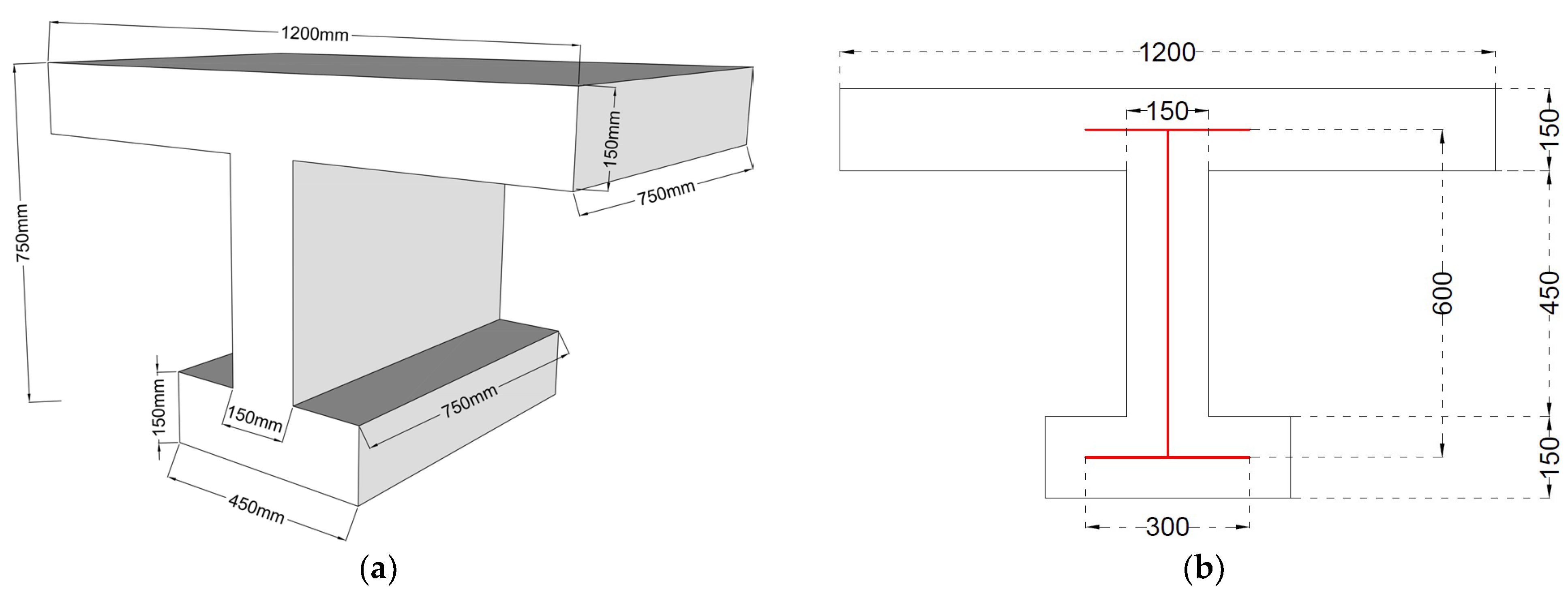
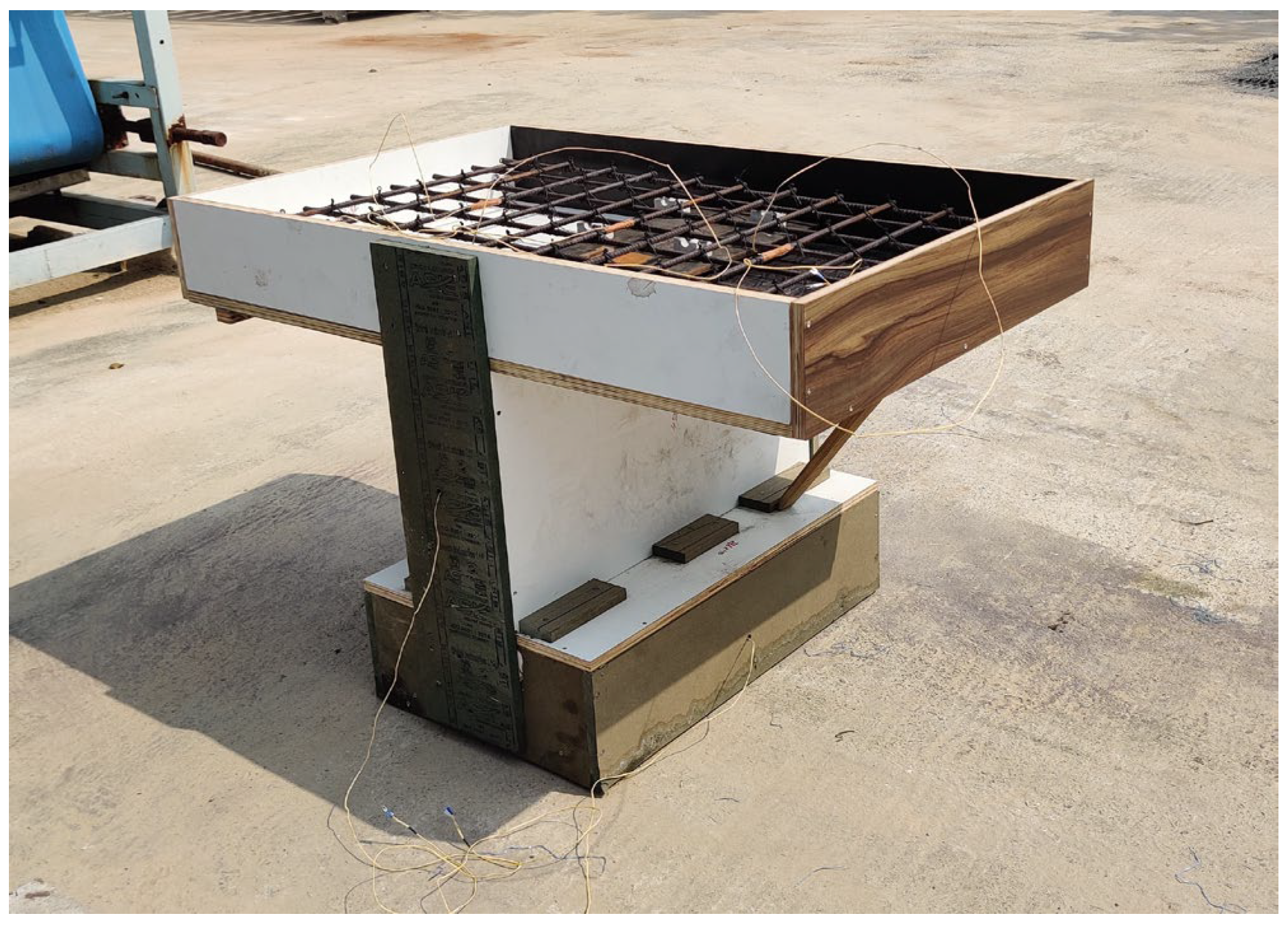
2.1. The Scale-Down Experimental Model of Concrete-Encased Steel I-Girder

The experimental concrete-encased steel I-girder segment has a top flange of width of 1200 mm, a bottom flange of 450 mm and a height of the web is 450 mm. Figure 1a shows the detailed dimensions of the I-girder. In this composite girder, a steel section is encased in the concrete section. The thickness of the steel section is 10 mm, which is fabricated as a steel beam where the flange width is 300 mm and the web is 600 mm respectively, which is shown in Figure 1b. Steel mesh of reinforcing bars 10 mm in diameter and 100 mm spacing in both directions was used to reinforce the girder’s top flange. Layers of plywood sheets were used to raise the girder off the ground to imitate the exact loading of ground-reflected radiation. Girder concrete has an average cube compressive strength of 47.25 MPa for 28 days.

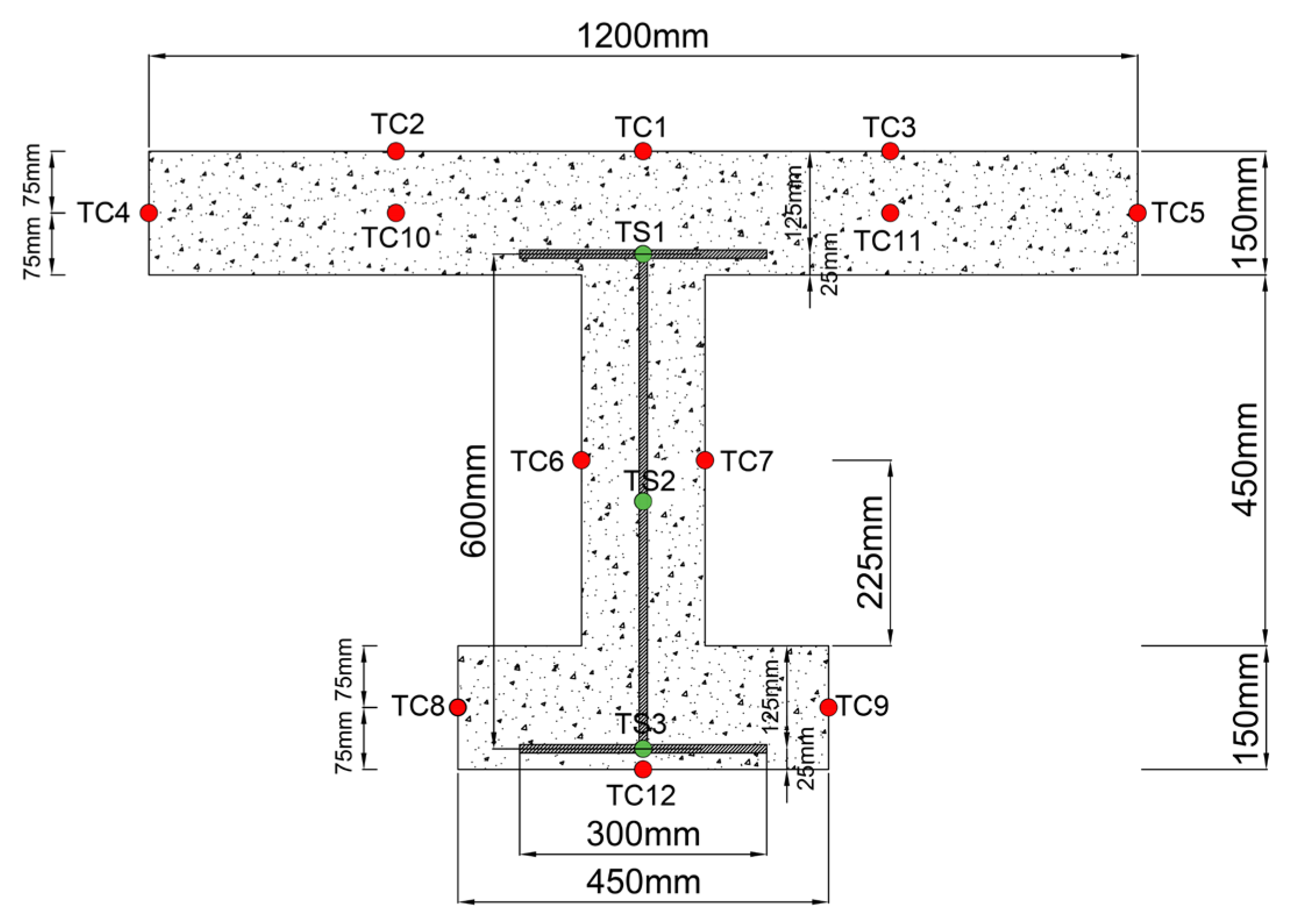
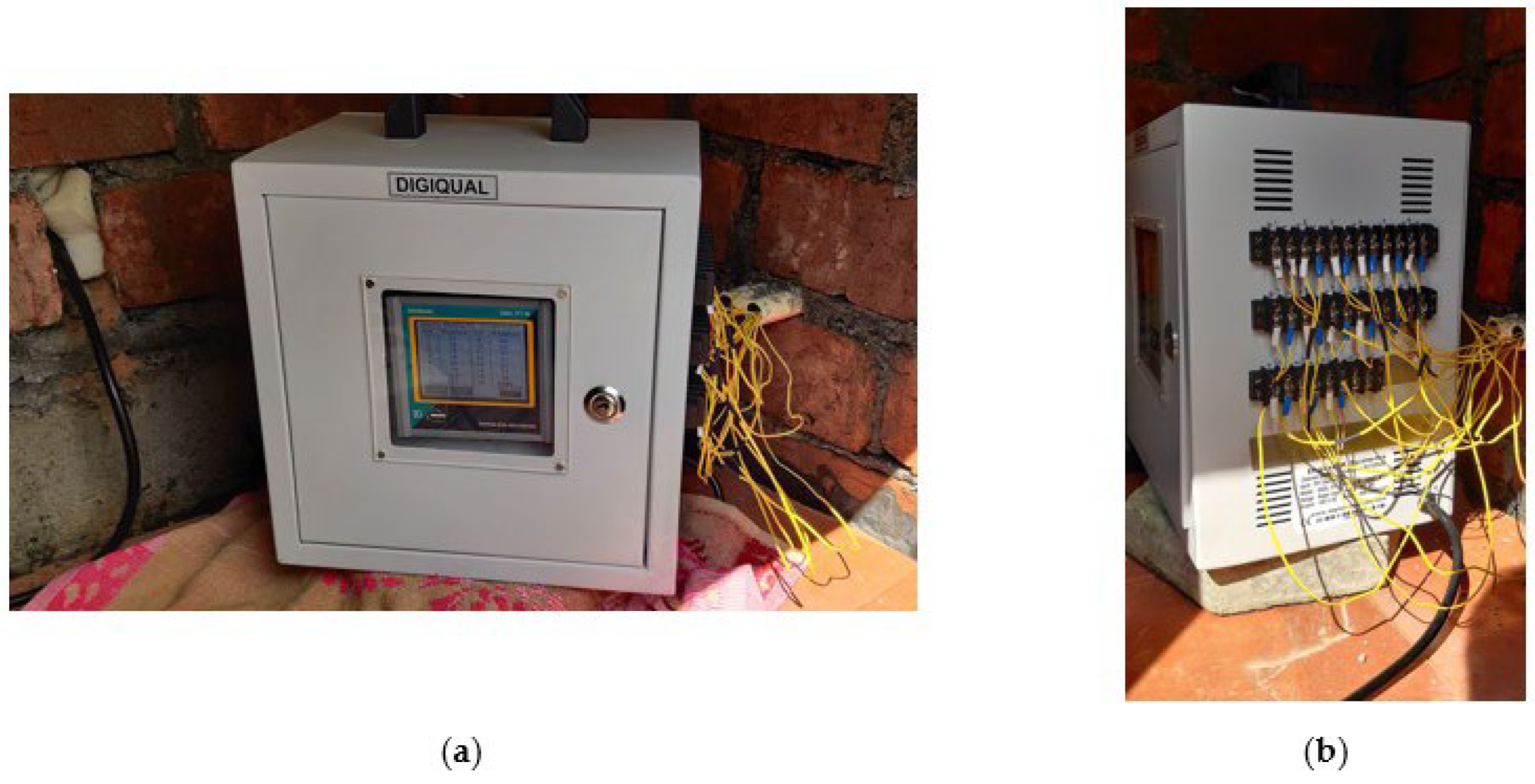
2.2. Distribution of Temperature Sensors in the Specimen

To keep records of the temperature variation in the concrete-encased steel I-girder, two groups of sensors were used in this experimental study. The first set included ambient thermal load sensors, which included a solar pyranometer to monitor the intensity of solar radiation measurement range of 0–1800 W/m². The second group of temperature sensors where Type-K thermocouples were installed in the mid-length section of the test specimen. The thermocouples were installed on the inside of the webs and flanges, as well as on the external and interior surfaces, to detect temperature variations in the concrete and steel. The coordinates of the thermocouples are shown in

Table 1. The thermocouple locations are indicated here.

Thermocouple	X Axis (mm)	Z Axis (mm)
TC1	0	750
TC2	−300	750
TC3	300	750
TC4	−600	675
TC5	600	675
TC6	−75	375
TC7	75	375
TC8	−225	75
TC9	225	75
TC10	−300	675
TC11	300	675
TC12	0	0
TS1	0	625
TS2	−5	350
TS3	0	25

and also shown in Figure 2. The thermocouples were grouped as TC and TS which indicates thermocouple in concrete and steel, respectively. 12 thermocouples are attached to the concrete portion and 3 thermocouples in steel beam. One group of thermocouples were attached to the steel section and also embedded in the concrete portion by tying on reinforcements where the remaining thermocouples were installed after casting which is shown in shown in Figure 3 and Figure 4. In Figure 5a,b, a data logger DQDL-96 multi-color touch screen paperless recorder is part of a larger data capture system that also incorporates thermocouple and solar pyranometer. Data from all sensors were gathered at 15-min intervals during the extreme cold season from the period of 1 November 2022 to 31 January 2023. Periodically, data collection has to be halted for reasons like power outages, system maintenance, and repairs during the estimated time.

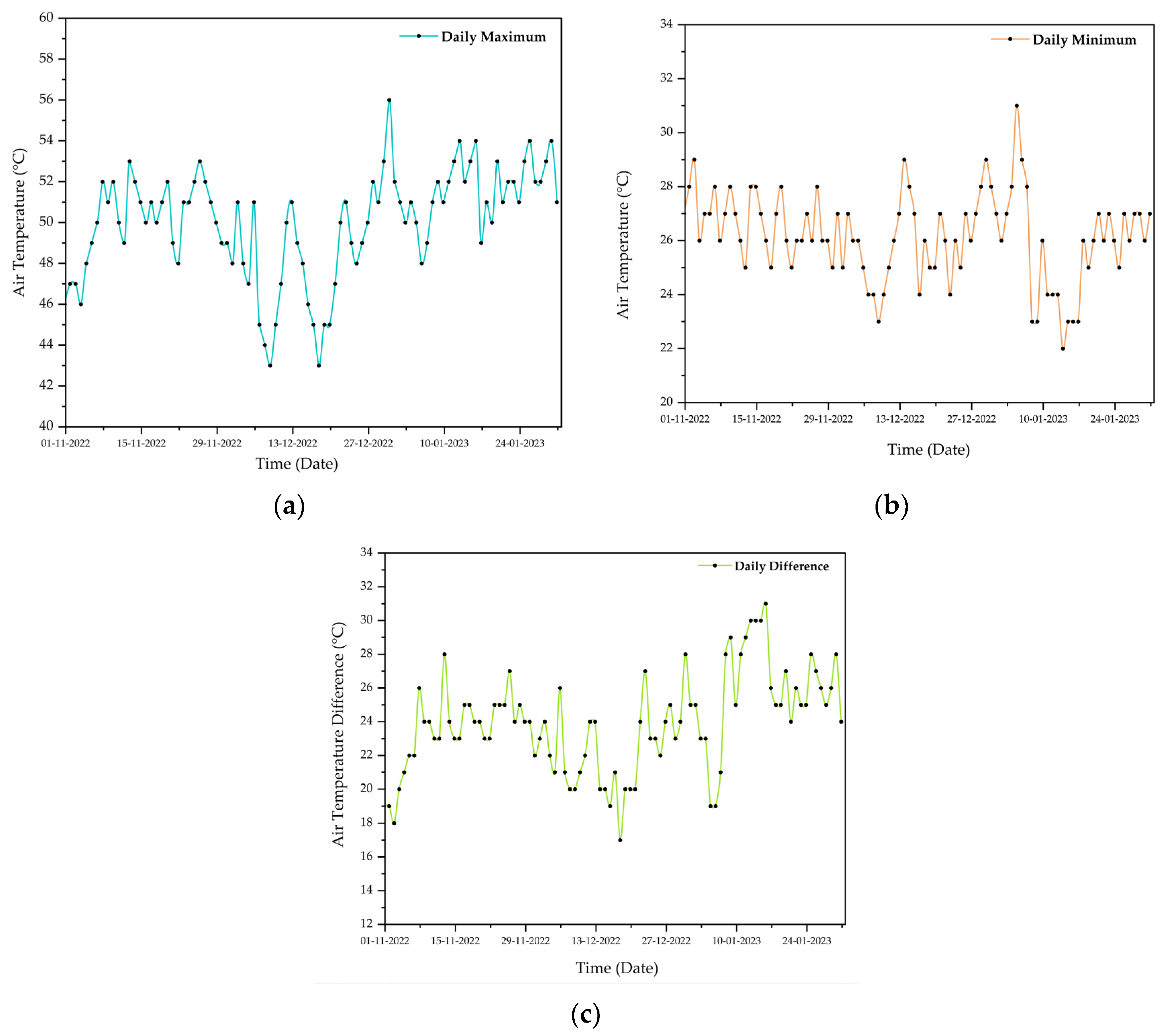
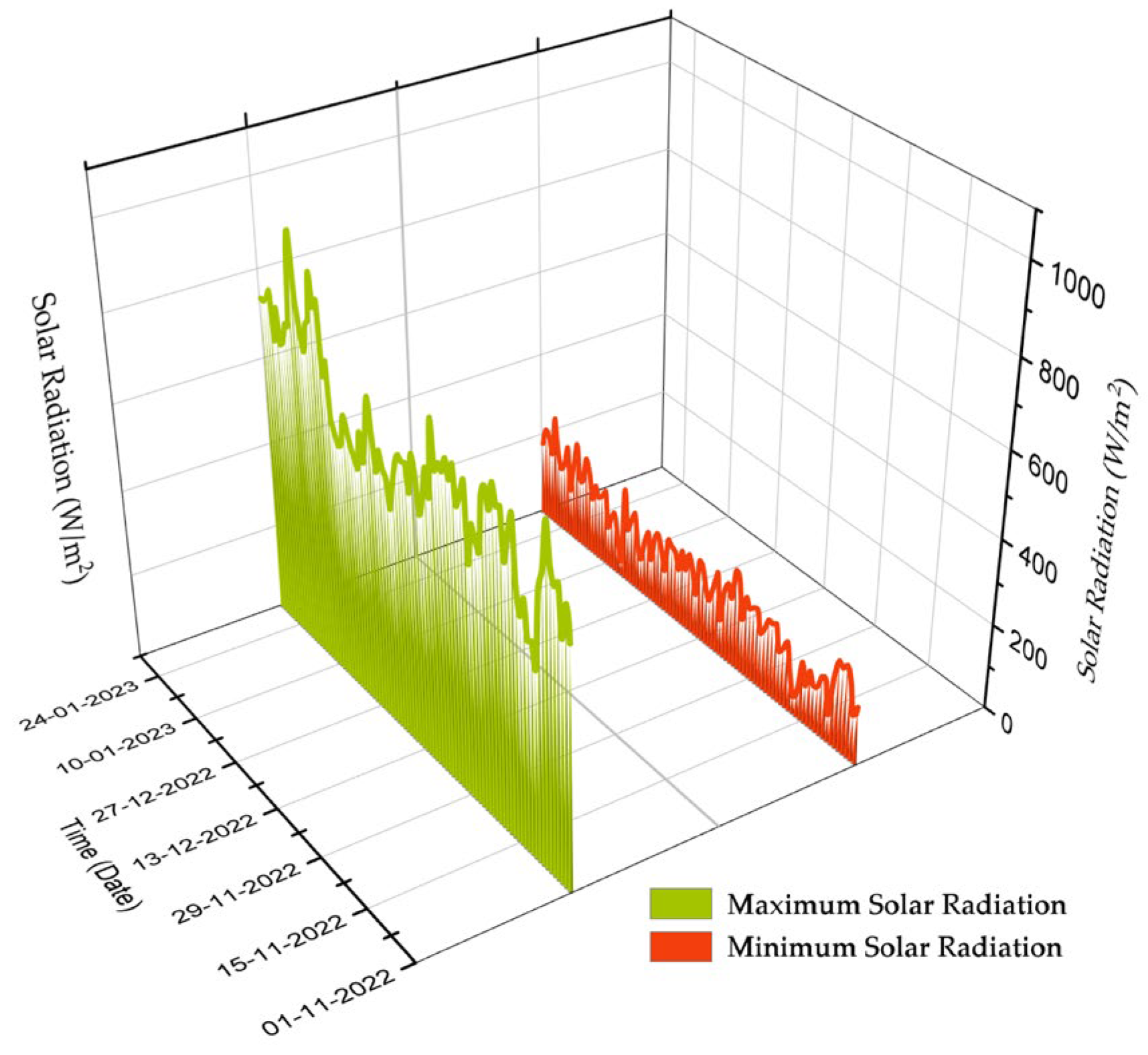
3. Air Temperature and the Solar Radiation during the Chosen Seasonal Period

This section showcases the environmental data we collected with our air temperature sensor and solar pyranometer. Consequently, the discussion of environmental data is necessary to comprehend the thermal response of the concrete-encased steel I-girder, as it is the thermal boundary loads that regulate the heat transfer within the girder. The data were recorded by using the data acquisition system depicts in Figure 5. Data logging during the extreme cold weather season involved recording the daily maximum and minimum temperatures and their variation. Analysis of the collected data revealed that the highest air temperature was 56 °C, which occurred on 31 December 2022, as presented in Figure 6a, and the minimum air temperature was 22 °C on 14 January 2023, as shown in Figure 6b. On the contrary side, the 16 January 2023, had the maximum daily temperature difference of 31 °C shown in Figure 6c.

Figure 6 depicts the maximum daily hourly global solar radiation tracked throughout the course of the time frame. The highest value recorded was 936 W/m² on 20 January 2023, however, there was noticeable variability in solar radiation on this day. Due to constant rain, daily minimum sun radiations of 34W/m² were observed on 6 January 2023, as shown in Figure 7.

4. Recorded Vertical and Lateral Temperature Gradients during the Selected Time Frame

4.1. Daily Recorded Maximum Temperature Gradients during the Selected Period

In this work, the phrase “temperature gradient” signifies the actual difference in temperature along a particular region. The daily maximum vertical and lateral temperature gradients recorded from 1 November 2022 to 31 January 2023 are shown in Figure. The temperature gradients were computed by subtracting the minimum temperature from the temperatures of all temperature sensors along the specific location. The vertical temperature gradients were computed using the midpoints of the webs connecting the upper and lower surfaces, and the lateral temperature gradients were computed using the midpoints of the top and bottom slabs. Maximum daily temperature variations for these portions were measured at the top layer for vertical gradients and the slab’s edge surfaces for lateral gradients. Simplified equations for predicting vertical and lateral temperature gradients may be derived from the daily maximum gradients and ambient thermal records for the above-mentioned time.

Solar radiation affects horizontal and vertical surfaces differently. The top slab of a structure is more affected than its webs, resulting in a significant increase in temperature during the day. Heat transfer is slow from the top surface to the web’s top section, resulting in high vertical temperature gradients. However, the temperature decreases significantly in the lower parts of the web, especially in the steel portion. Lateral temperature gradients along the slabs are greater than along the web during this period.

4.2. Vertical and Lateral Daily Temperature Gradients in Selected Period

Based on the thermal records, 3 days were chosen from the selected period which represents the maximum temperature variations on the vertical and lateral sides of the I-Girder. During these days, the observed thermal radiations on the steel section were also discussed. Based on the records, one day has been selected for every month where the maximum temperature gradient was observed on the 10 November 2022, 31 December 2022, and 16 January 2023. Figure 8a shows that the daily maximum vertical temperature gradients along the south web were significant in November and minimal on many of these days in December. During the winter, the sun’s rays strike at low solar altitude angles, warming just one edge of the horizontal members while shadows are cast on the other. The lateral temperature gradients in the top slabs are notably higher than those in the bottom slabs. Figure 8b,c illustrates the maximum observed thermal gradients are normally higher in the lateral gradient than the vertical gradient. The top flange observed maximum temperature values which are slightly higher than the bottom flange, south and north side of the web member in the I-girder.

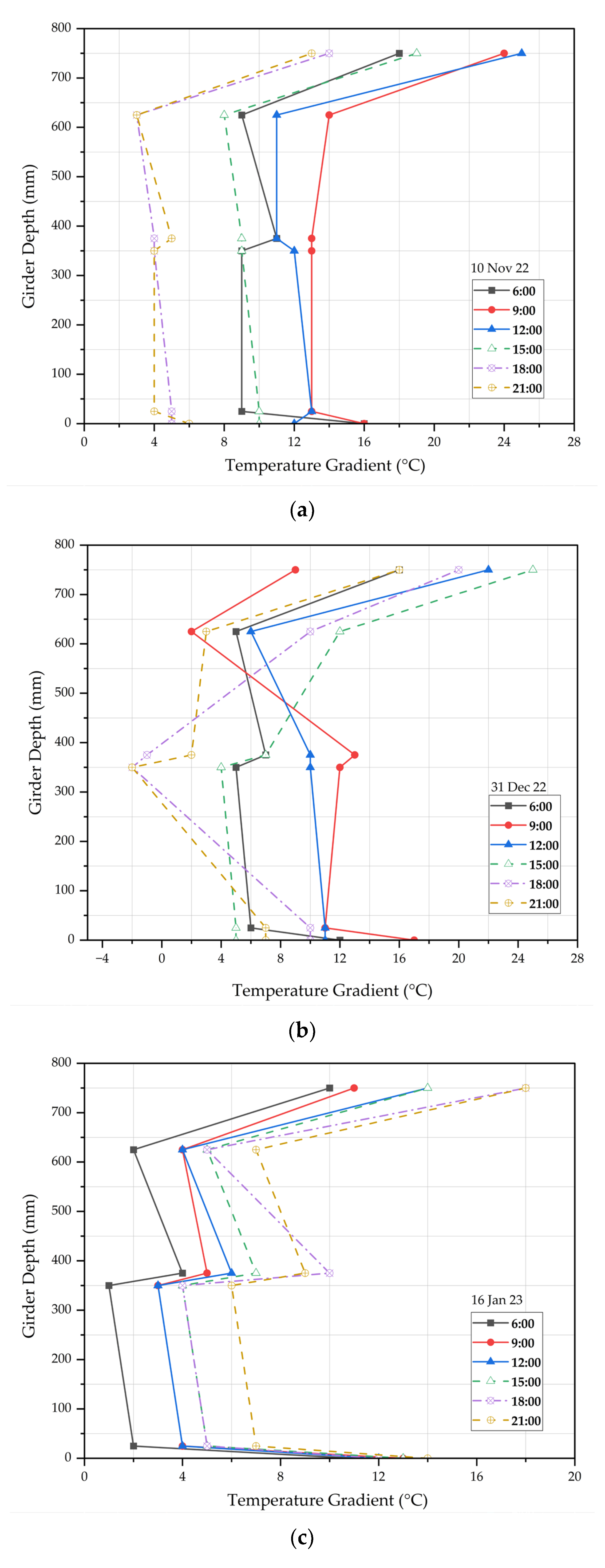
4.3. Vertical Daily Thermal Gradient Distributions on the I-Girder

Figure 9 and Figure 10 clearly show that the lateral gradients (TS & BS) were maximum than the vertical gradients. Figure 9a for 10 November 2022, Figure 9b for 31 December 2022, and Figure 9c for 16 January 2023, which depicts the temperature gradient variation throughout the girder depth at various intervals of time ranging from 6:00 to 21:00 h. The temperature gradient reaches its maximum on 10 November 2022, as solar radiation begins to perk up the girder after daylight. At 6:00, which is an hour after daylight, the vertical gradient is nearly uniform in the mid and bottom sections of the girder, with the top surface being warmer than the interior of the web. By 9:00, the influence of sun radiation becomes more apparent, with the top portion much warmer. The gradient distribution at 12:00 shows the most significant positive gradients during the middle of the day, and this phenomenon persists. As the sun descends, the temperature of the upper surface decreases, resulting in a reduction in temperature gradients over time, as shown in the distributions at 15:00 and 18:00. Although the top surface temperature decreases during the night, the interior of the girders retains most of the heat transferred during the daytime.

Figure 8a illustrates these changes in temperature gradient over time. In Figure 9, the reason for the large temperature difference is due to the thermocouple location where the thermocouple at 375 mm is at the outer surface of the concrete which has more exposure to solar radiation and in the location 350 mm which is in the innermost part of the web portion. Sometimes the time of the day also decides the temperature variation between the thermocouple locations. Equivalent variations in the vertical temperature gradients occurred on 31 December 2022, as shown in Figure 9b, although with minor deviations. The negative gradient values are detected in the mid portion of the web between 18:00 and 21:00 on December 25, which was not identified on 10 November. On 31 December, the gradients were smaller compared to those on 10 November, and the gradients at the bottom portion were found smaller than those at the top portion. In contrast, on 16 January 2023, the positive gradients at the top surface were found to be too small compared to those on 31 December and 10 November. However, the mid-surface gradients were approaching the negative gradients, although they were still greater than those on 31 December.

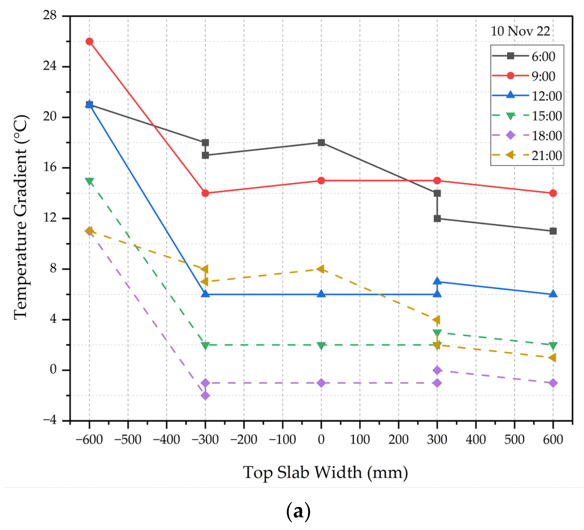
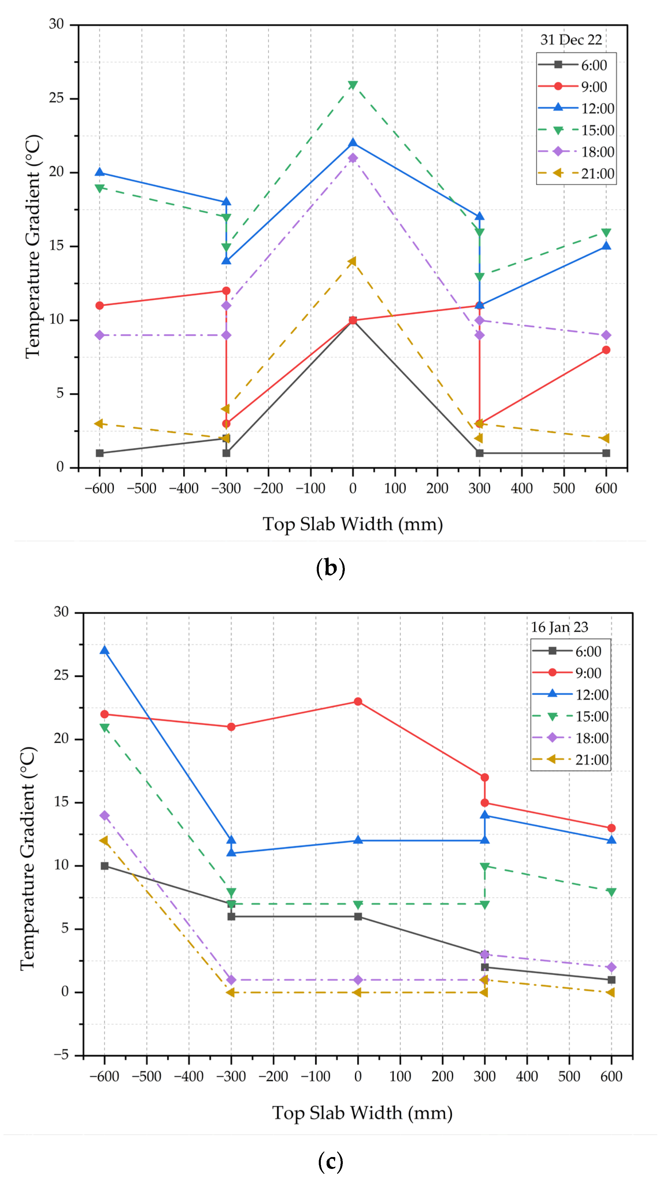
4.4. Lateral Daily Thermal Gradient Distributions on the I-Girder

The sun rises in the southeast in the winter and continues to move to the south of the equatorial plane, the temperature on the southern edge of the top flange is always greater than that on the northern edge during the day. This is because the sun is moving southward. Figure 10a for 10 November 2022, Figure 10b for 31 December 2022, and Figure 10c for 16 January 2023 illustrated the temperature gradient variation along the top flange of the girder at different time intervals ranging from 6:00 to 21:00. During the entire day, the temperature on the southern edge of the top flange is invariably likely to be greater than the temperature on the northern edge. In addition, the only thermocouples that encounter significant changes in the gradient are those positioned along the edges. Due to the solar radiation after sunrise, the temperature gradient on the edges gradually increases from 6:00 to 12:00, then it falls from there till 21:00 h.

Figure 10a,b clearly shows that the lateral temperature gradients are comparatively higher at 21:00 than in the early hours of the day due to the heat transfer. Due to the solar radiation after sunrise, the temperature gradient on the edges gradually increases from 6:00 to 12:00 then it falls from there until 21:00 hrs. The highest temperature gradients observed at the edges of the girder were 26 °C, 24 °C, and 20 °C on 10 November, 31 December, and 23 January respectively. The negative temperature gradient was identified between November and January at 18:00 and 21:00 in the top flange’s middle part, as shown in Figure 10a,c. In Figure 10 Lateral temperature gradient distributions at different intervals (a) on 10 November 2022, (b) on 31 December 2022, and (c) on 16 January 2023, the abrupt temperature changes at −300 and +300 are due to the thermocouple location where at both −300 and +300, there are two thermocouples were installed at the height of 675 mm and 750 mm. The thermocouple at the zone 750 mm is constantly exposed to direct solar radiation whereas the thermocouple at 675 mm is winded in the innermost part of the top slab. Due to this, the temperature changes are observed at the locations −300 and +300 in the top slab.

5. Correlations between Experimental Data

In this chapter, experimental observations from temperature sensors and a monitoring system are employed to test the correlations between ambient thermal loads and lateral and vertical temperature gradients. Using the formulae derived from the proposed study’s experimental results, the maximum temperature gradient at the top layer of a concrete-encased steel I-girder may be estimated for any region and all weather conditions. Likewise, the maximum lateral temperature gradients at the top and bottom slab edges are determined by using the derived lateral gradient formulas.

The suggested equations were validated using the coefficient of determination and two additional error measures (R²). Root-mean-square error (RMSE) and Mean absolute error (MAE) were applied as the error measurement techniques:

$$\mathrm{RMSE}=\sqrt{\frac{ {\mathit{\sum }(X_{pre}-X_{exp})}^2}{n}}$$

(1)

$$\mathrm{MAE}=\frac{ \mathit{\sum }(X_{pre}-X_{exp})}{n}$$

(2)

In this equation, X_pre represents the forecast, X_exp represents the historical experimental values at comparable intervals, and where ‘n’ represents the sum of all the records.

5.1. Determination of Vertical Temperature Gradient

5.1.1. Correlations Analysis with Thermal Loads

Furthermore, substantial variability in solar radiation was reported on several days due to cloud cover fluctuation and power failures due to maintenance. These periods’ data were not taken into account in the computations. Cracks and deformations in the structure may emerge as a result of thermal stresses caused by nonlinear temperature distributions along the cross-section. To maintain the bridge’s long-term stability, designers must carefully consider the temperature differences along the web.

Table 2. Empirical formulae for the vertical thermal gradients.

Articles Discussed	Empirical Equation	Location
Potgieter and Gamble [11]	$TD=28.2|\frac{I_d\alpha }{28.09}-0.7|+0.342\left(T_d-11.1\right)+VV$	Illinois, USA
Roberts-Wollman et al. [1]	$TD=0.9\left(T_{max}-T_{3a}\right)+0.56\left(I_d-12\right)$	Texas, USA
Lee and Kalkan. [5]	$TD=\frac{3I_d}{4}+\frac{\left(T_{max}-T_{min}\right)}{15}-\left(0.37+2.93w-0.25w^2+0.008w^2\right)$	Georgia, USA
Abid et al. [9]	$TD=2.57+0.181T_d+\left(0.534I_d-0.0027I_d{}^2\right)-\left(1.32w-0.21w^2\right)$	Gaziantep, Turkey
Sheng, Zhou, Huang, Cai, & Shi [16]	$TD=9.35+0.299T_d+0.0492I_d+0.0237I_d{}^2-0.0005I_d{}^3-1.8925w+0.0893w^2$	25

details the results of various statistical and experimental investigations on temperature gradients of bridge girders [1,5,9,11,15] that resulted in the formulation of certain standard empirical equations relying on meteorological parameters. Here, we discuss and compare formulas from the literature that predict the maximum vertical temperature gradient from the daily temperature differential (DT) in degrees Celsius, the daily total solar radiation (I) in megajoules per square metre, and the daily average wind speed (w) is ignored in this study due to its minimal impact in that location.

5.1.2. Vertical Temperature Gradient Formula Prediction

Initially, a step—by—step regression was performed using DT, I, w, the average daily temperature variation over three days (3DT) in degrees Celsius, the average daily maximum and minimum temperatures over the same time period (Tmax and Tmin), the average daily total solar radiation over the same time period (MJ/m2), and the average daily maximum hourly solar radiation over the same time period (Imax and I). Based on the experimental records, an empirical realtion was derived based on the reference from Table 2. Roberts-Wollman [1] developed a simpler equation in 2002 to forecast the maximum vertical temperature gradient based on the daily maximum air tem-perature (Tmax), the three-day average air temperature (3Tave), and the daily total solar radiation (I). This demonstrates the high degree of reliability with which the suggested formula may be employed to measure the maximum vertical temperature gradient of the given I-girder.

5.2. Lateral Temperature Gradients

Despite the fact that lateral temperature differences along slabs have a substantial impact on transverse thermal deformations and stresses of box-girders, the study on this topic is restricted. The temperature gradients of the top and bottom flanges were estimated using the lateral temperature distributions along the centerlines of the top and bottom slabs (BS). As with the vertical temperature gradient, stepwise regression analysis was performed as an early step to determine the degree of effect of each parameter and to identify simplified equations with high determination coefficients. The proposed formula is highly correlated with the experimental measurements with R² of 0.97 which is shown in Figure 11.

Predicted TF and BF Vertical Temperature Gradient Formula

Figure 12 depicts the relationship between the predicted and observed daily maximum lateral thermal gradients of the top slab (TS). The figure shows that the projected values are highly linked with their corresponding experimental values. The forecasted formula shows a high degree of correlation, with an R² of 0.90, and the MAE and RMSE were 0.46 and 0.57, respectively. The figure depicts the relationship between the predicted and observed daily maximum lateral thermal gradients of the bottom slab (BS). The figure shows that the projected values are highly linked with their corresponding experimental values. The forecasted formula shows a high degree of correlation, with an R² of 0.94, and the MAE and RMSE were 0.37 and 0.47, respectively which is shown in

Table 3. Correlation comparisons of the current and previous study of Ver.

Experimental Studies	R2	RMSE	MAE
Potgieter and Gamble [11]	0.81	5.28	4.95
Roberts-Wollman et al. [1]	0.94	3.54	2.93
Lee and Kalkan. [5]	0.95	2.47	1.99
Abid et al. [9]	0.96	0.78	0.65
Current study	0.97	0.35	0.28

.

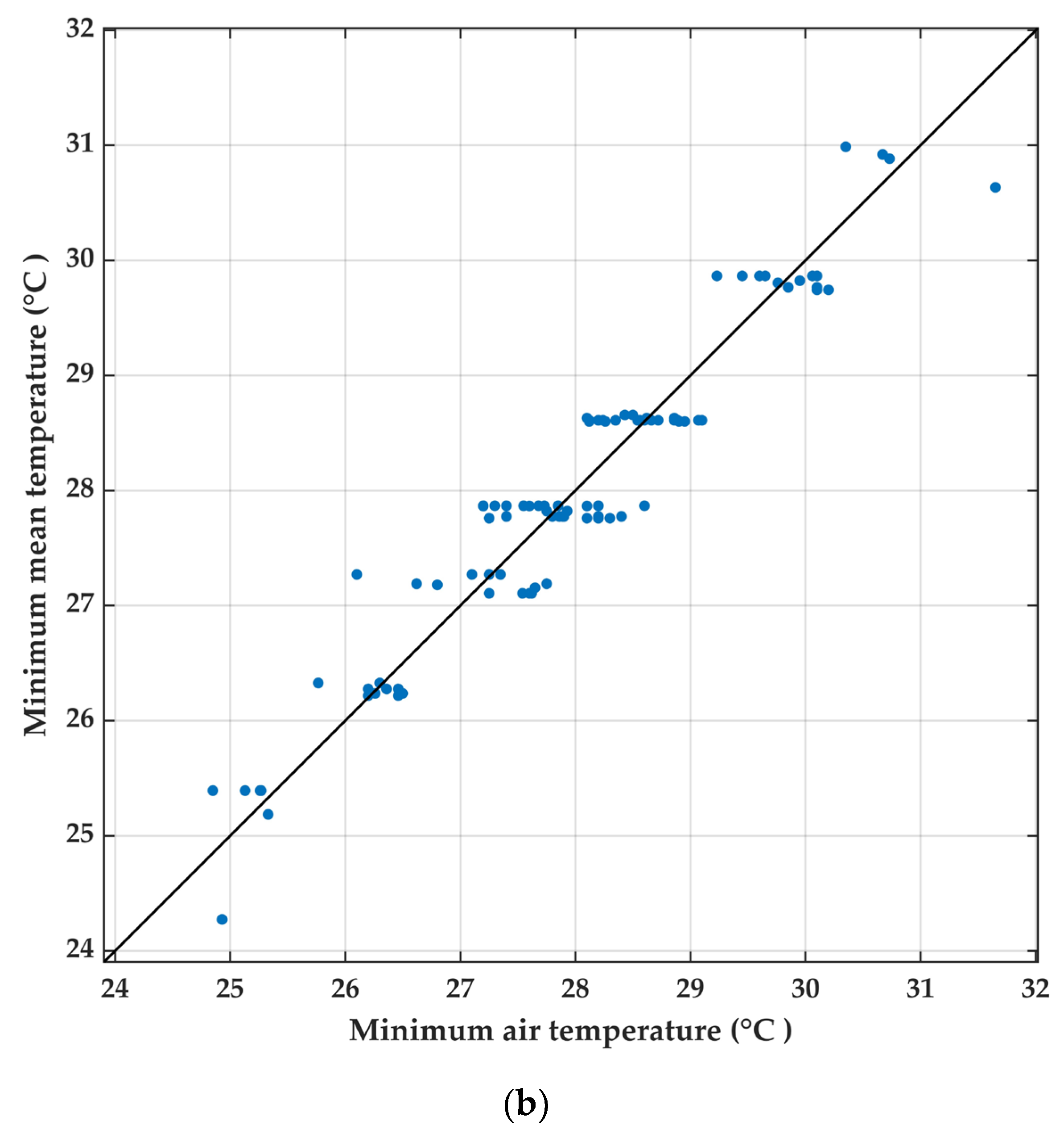
6. Mean Temperature of the Girder

Following stepwise regressions with several environmental parameters, the maximum daily mean temperature of the girder MeanT_max was shown to be quite significantly linearly linked to the daily maximum air temperature T_max, as shown in Figure 13a. Similarly, the linear connection between the daily minimum mean temperature of the girder Mean T_min and the daily minimum air temperature T_min was extremely good, as illustrated in Figure 13b. The suggested equations R² values for MeanT_max and MeanT_min were 0.86 and 0.92, respectively.

$$Mean{T}_{max}=0.64T_{max}+8.731$$

(3)

$$Mean{T}_{min}=0.87T_{min}+5.283$$

(4)

7. Conclusions

The experimental data was observed from 1 November 2022 to 31 December 2023 during the extreme cold season. This experiment examined how girder size impacts temperature trends in concrete-encased steel girders. The results were used to develop an empirical equation using stepwise regression analysis. The purpose of the experiment was to ascertain the lateral and vertical thermal profiles within the girders:

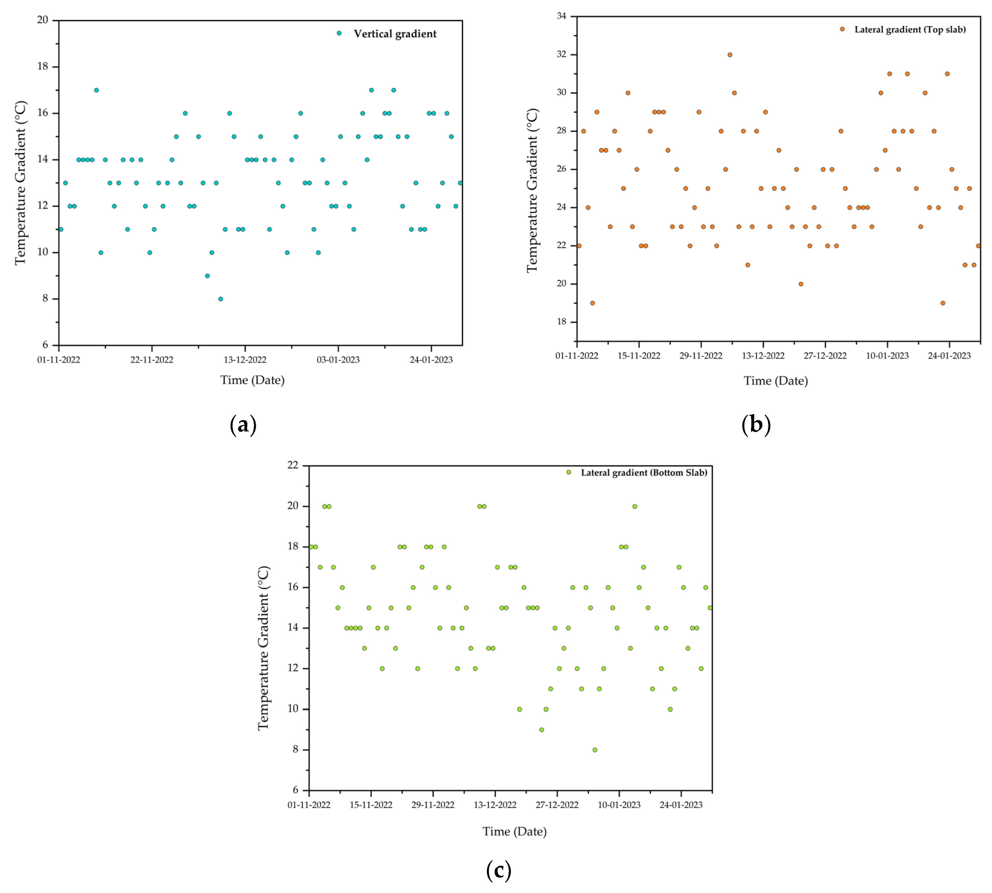
• In November, the sun’s rays hit the top surface of the I-girder at a high angle, causing solar radiation to focus on that area during the hottest part of the day. Due to this effect, the temperature of the topmost fibers was higher than the temperature of fibers located at other heights on the girder, which created higher vertical temperature gradients than during other months. Throughout the period of observation, the maximum vertical temperature gradients recorded on 10 November 2022, 16 January 2023, and 26 December 2022 were 17 °C, 17 °C, and 16 °C, respectively, regardless of the month.
• Conversely, during winter, the sun’s rays hit vertical surfaces with greater intensity than horizontal surfaces due to the low altitude angles of the sun’s rays. Furthermore, during the winter season, the sun’s movement leads to higher intensity of solar radiation on the southern edges compared to the northern edges. As a consequence, more significant lateral thermal gradients are observed across the slabs in the mentioned time frame, with a greater magnitude compared to other seasons. Similarly, the maximum lateral temperature gradients in the top slab of the girder for each month observed were 32 °C, 30 °C, and 31 °C on 13 November 2022, 6 December 2022, and 11 January 2023, respectively. The highest lateral temperature gradients in the bottom flange of the girder for every month recorded on 5 November 2022, 11 December 2022 and 14 January 2023 were 20 °C, 20 °C, and 19 °C, respectively.
• The predicted temperature gradients were compared to earlier empirical calculations. To forecast the peak vertical temperature gradient of the I-girder over various locations in the near future, mathematical equations with correction coefficients were developed based on parametric research.
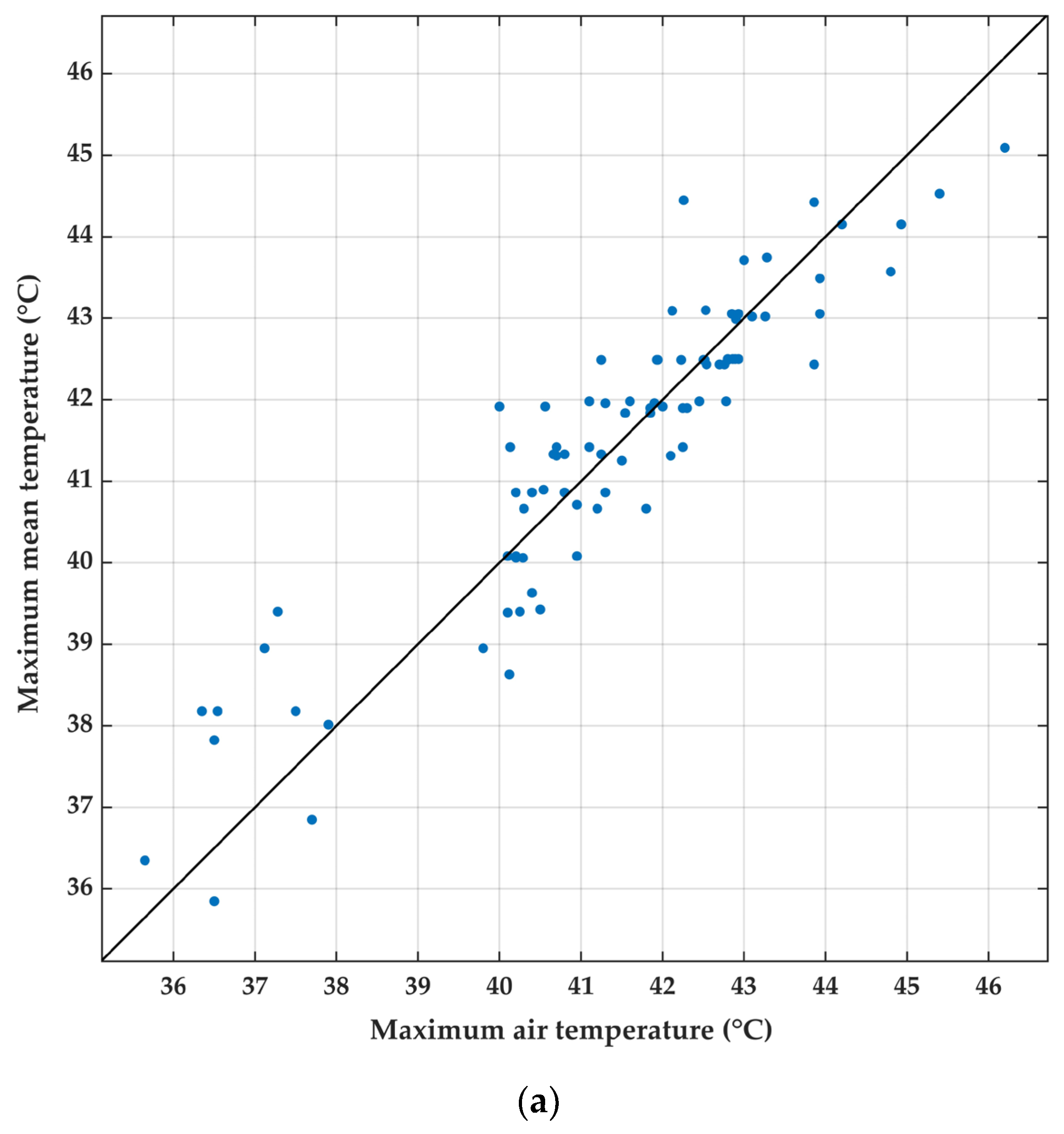
• Based on the linear correlation and regression analysis, the relationship between MT_max and T_max had an R² value of 0.85, and the relationship between MT_min and T_min had an R² value of 0.93.
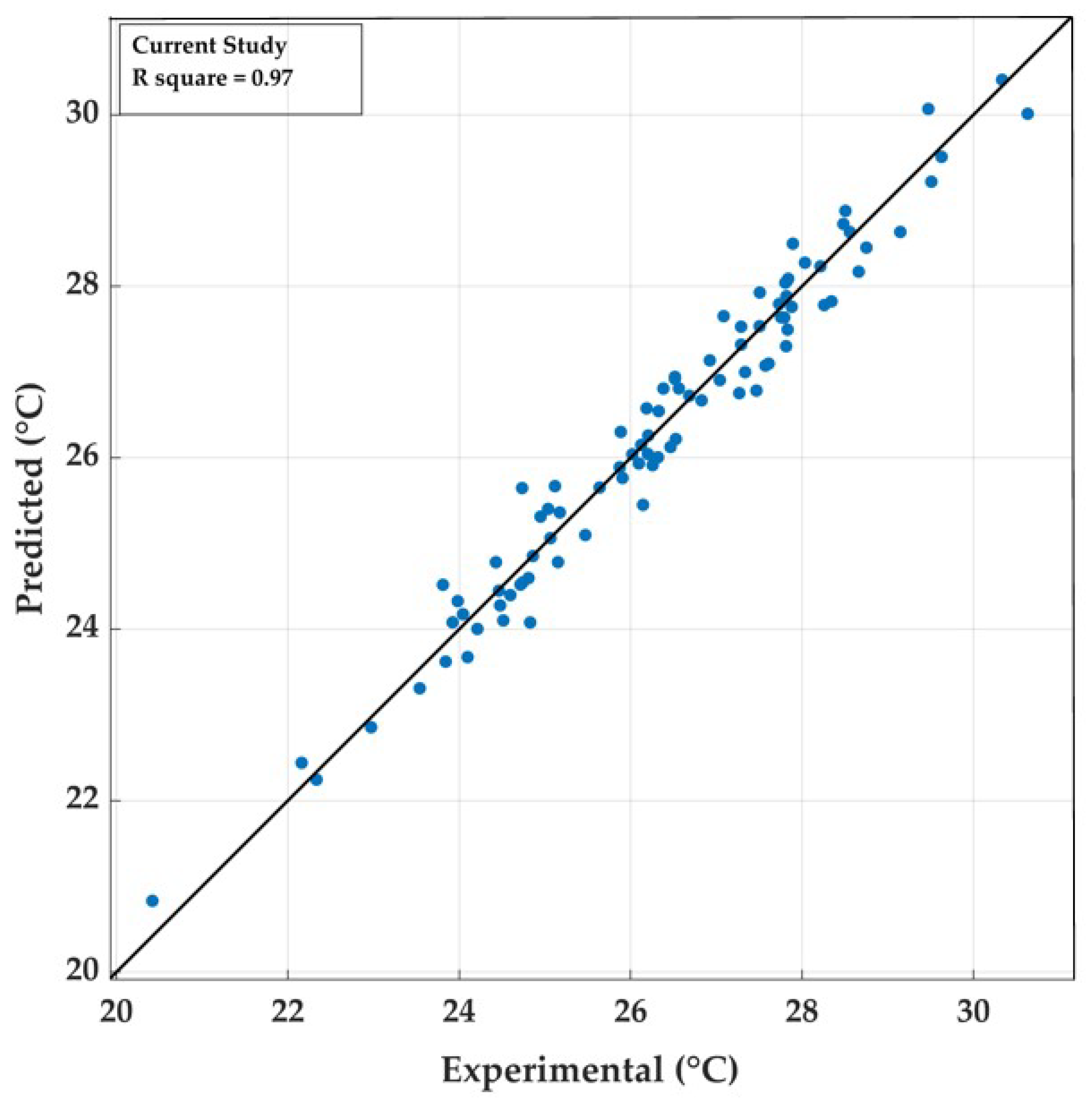
• Compared to previous formulas, the newly proposed formula exhibited superior performance, with the highest coefficient value of 0.97 and minimal errors. The results showed a strong correlation between the proposed formula and the experimental measurements.
• Formulas were adopted empirically to evaluate the peak lateral temperature gradients at the top and bottom portions, akin to the vertical thermal gradient. The R² values for the anticipated lateral temperature gradient equations for the top slab and bottom slab were 0.90 and 0.94, respectively.

References

1. Roberts-Wollman, C.L.; Asce, M.; Breen, J.E.; Asce, F.; Cawrse, J. Measurements of Thermal Gradients and their Effects on Segmental Concrete Bridge. J. Bridg. Eng. 2002, 7, 166–174. [Google Scholar] [CrossRef]
2. Imbsen, R.A.; Vandershaf, D.E.; Schamber, R.A.; Nutt, R.V. Thermal Effects in Concrete Bridge Superstructures; National Cooperative Highway Research Program: Washington, DC, USA, 1985; ISBN 030903860X.
3. Lee, J. Investigation of Extreme Environmental Conditions and Design Thermal Gradients during Construction for Prestressed Concrete Bridge Girders. J. Bridg. Eng. 2012, 17, 547–556. [Google Scholar] [CrossRef]
4. Zhang, C.; Liu, Y.; Liu, J.; Yuan, Z.; Zhang, G.; Ma, Z. Validation of long-term temperature simulations in a steel-concrete composite girder. Structures 2020, 27, 1962–1976. [Google Scholar] [CrossRef]
5. Lee, J.-H.; Kalkan, I. Analysis of Thermal Environmental Effects on Precast, Prestressed Concrete Bridge Girders: Temperature Differentials and Thermal Deformations. Adv. Struct. Eng. 2012, 15, 447–460. [Google Scholar] [CrossRef]
6. Ho, M.; Lau, K.; Tian, Z.; Graves, Y.J. Open Field Temperature and Strain Records of a Concrete-Steel Composite Beam Open Field Temperature and Strain Records of a Concrete- Steel Composite Beam. IOP Conf. Ser. Mater. Sci. Eng. 2021, 1090, 012107. [Google Scholar] [CrossRef]
7. Elbadry, M.; Ghali, A. Thermal Stresses and Cracking of Concrete Bridges Thermal Stresses and Cracking of Concrete Bridges. J. Proc. 1986, 83, 1001–1009. [Google Scholar]
8. Kim, S.; Park, S.; Wu, J.; Won, J. Temperature variation in steel box girders of cable-stayed bridges during construction. J. Constr. Steel Res. 2015, 112, 80–92. [Google Scholar] [CrossRef]
9. Abid, S.R.; Tays, N.; Özakça, M. Experimental analysis of temperature gradients in concrete box-girders. Constr. Build. Mater. 2016, 106, 523–532. [Google Scholar] [CrossRef]
10. Tayşi, N.; Abid, S. Temperature Distributions and Variations in Concrete Box-Girder Bridges: Experimental and Finite Element Parametric Studies. Adv. Struct. Eng. 2015, 18, 469–486. [Google Scholar] [CrossRef]
11. Potgieter, I.C.; Gamble, W.L. Response of Highway Bridges to Nonlinear Temperature Distributions; University of Illinois at Urbana-Champaign: Champaign, IL, USA, 1983. [Google Scholar]
12. American Association of State Highway and Transportation Officials. AASHTO LRFD Bridge Design Specifications; American Association of State Highway and Transportation Officials: Washington, DC, USA, 2012; ISBN 9781560515234. [Google Scholar]
13. Feng, Z.; Liu, J.; Gao, L. Experimental investigation of temperature gradients in a three-cell concrete box-girder. Constr. Build. Mater. 2022, 335, 127413. [Google Scholar] [CrossRef]
14. Abid, S.R.; Tayşi, N.; Özakça, M.; Xue, J.; Briseghella, B. Finite element thermo-mechanical analysis of concrete box-girders. Structures 2021, 33, 2424–2444. [Google Scholar] [CrossRef]
15. Sheng, X.; Zhou, T.; Huang, S.; Cai, C.; Shi, T. Prediction of vertical temperature gradient on concrete box-girder considering different locations in China. Case Stud. Constr. Mater. 2022, 16, e01026. [Google Scholar] [CrossRef]
16. Abid, S.R.; Al-Gasham, T.S.; Xue, J.; Liu, Y.; Liu, J.; Briseghella, B. Geometrical Parametric Study on Steel Beams Exposed to Solar Radiation. Appl. Sci. 2021, 11, 9198. [Google Scholar] [CrossRef]
17. Guo, F.; Zhang, S.; Duan, S. Analysis of Measured Temperature Field of Unpaved Steel Box Girder. Appl. Sci. 2022, 12, 8417. [Google Scholar] [CrossRef]
18. Abid, S.R.; Mussa, F. Experimental and finite element investigation of temperature distributions in concrete-encased steel girders. Struct. Control Health Monit. 2022, 25, 8–10. [Google Scholar] [CrossRef]
Figure 1. Geometry of the concrete encased steel I girder segment should be listed as: (a) 3D perspective of the girder; (b) Sectional view of a girder’s cross-section.
Buildings 13 00780 g001
Figure 2. Location of the distributed sensors on the girder segment.
Buildings 13 00780 g002
Figure 3. The scale-down experimental model of I-girder segment Formwork and temperature sensors spaced around the top flange.
Buildings 13 00780 g003
Figure 4. Distributed sensors on the girder segment.
Buildings 13 00780 g004
Figure 5. Data acquisition system for temperature measurements: (a) Observed readings during the temperature study; (b) Thermocouple wires connections with the data logger.
Buildings 13 00780 g005
Figure 6. Air temperature data for daily timeframes from 1 November 2022 to 31 January 2022 (a) Daily maximum (b) Daily minimum (c) Daily difference.
Buildings 13 00780 g006
Figure 7. Daily maximum hourly solar radiation from 1 November 2022 to 31 January 2022.
Buildings 13 00780 g007
Figure 8. Daily maximum recorded temperature gradients during 1 November 2022 to 31 January 2023: (a) vertical gradient running across the webs, (b) top slab lateral gradient, and (c) lateral gradient flowing in the bottom slab.
Buildings 13 00780 g008
Figure 9. Vertical temperature gradient distributions at different intervals (a) in 10 November 2022, (b) in 31 December 2022, and (c) in 16 January 2023.
Buildings 13 00780 g009
Figure 10. Lateral temperature gradient distributions at different intervals (a) in 10 November 2022, (b) in 31 December 2022, and (c) in 16 January 2023.
Buildings 13 00780 g010aBuildings 13 00780 g010b
Figure 11. Predicted daily peak vertical temperature gradient for the present research.
Buildings 13 00780 g011
Figure 12. The greatest possible lateral temperature gradient anticipated each day for present research work (a) top slab, and (b) bottom slab.
Buildings 13 00780 g012
Figure 13. Daily mean girder temperature: (a) maximum mean vs. maximum air temp, (b) minimum mean versus minimum air temp.
Buildings 13 00780 g013aBuildings 13 00780 g013b