
On the Thermal Environmental Quality of Typical Urban Settlement Configurations


Abstract
:1. Introduction
2. Materials and Methods
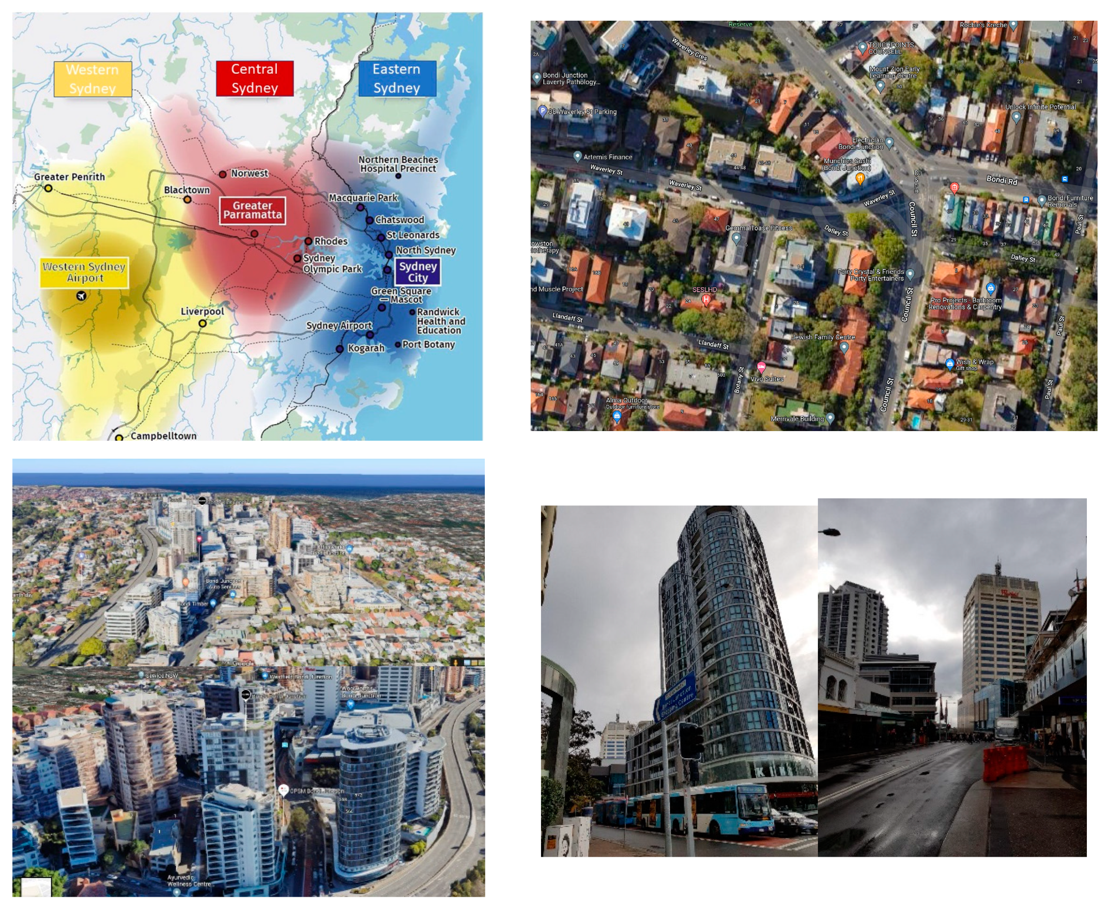
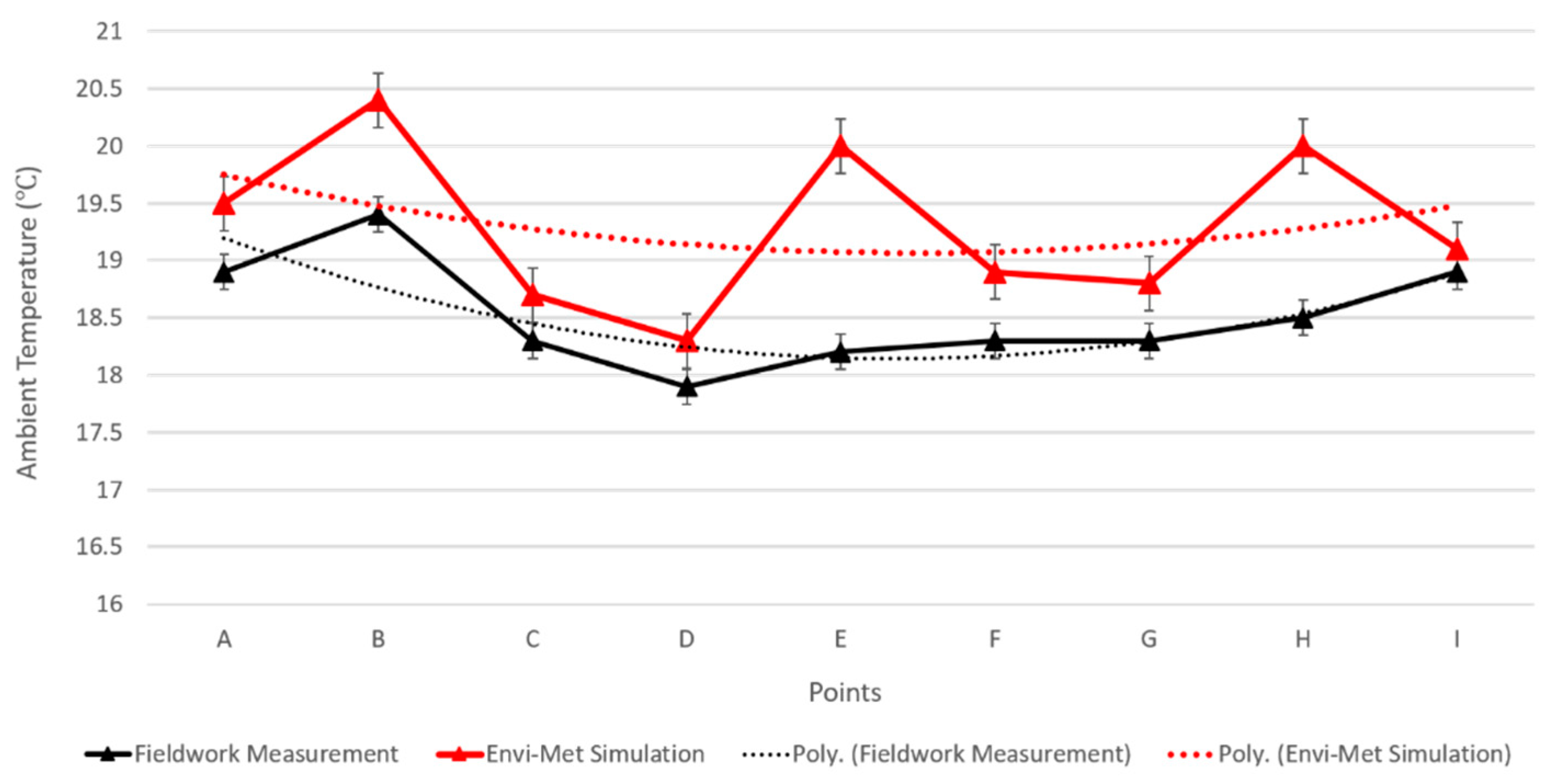
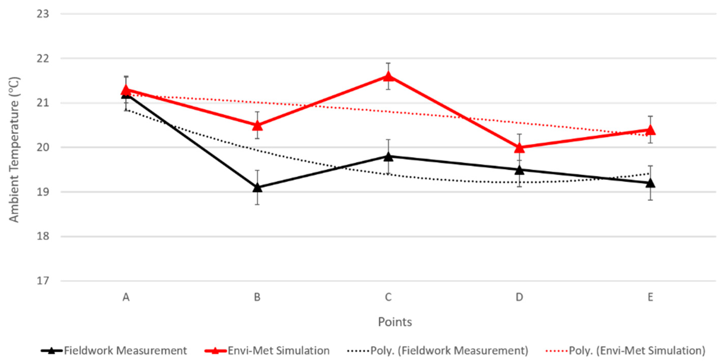
2.1. Field Measurement
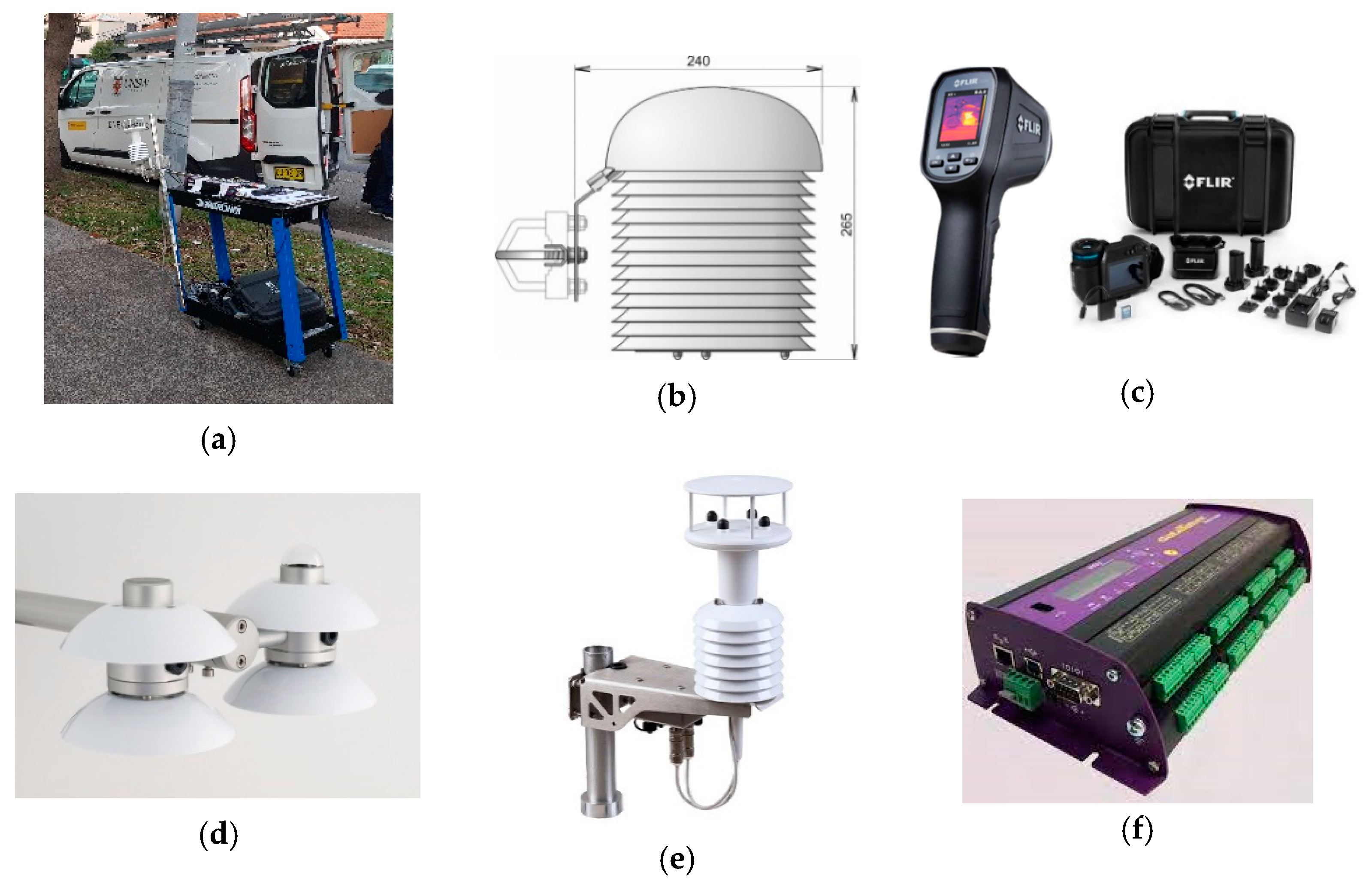
2.2. Instruments and Measurement Techniques
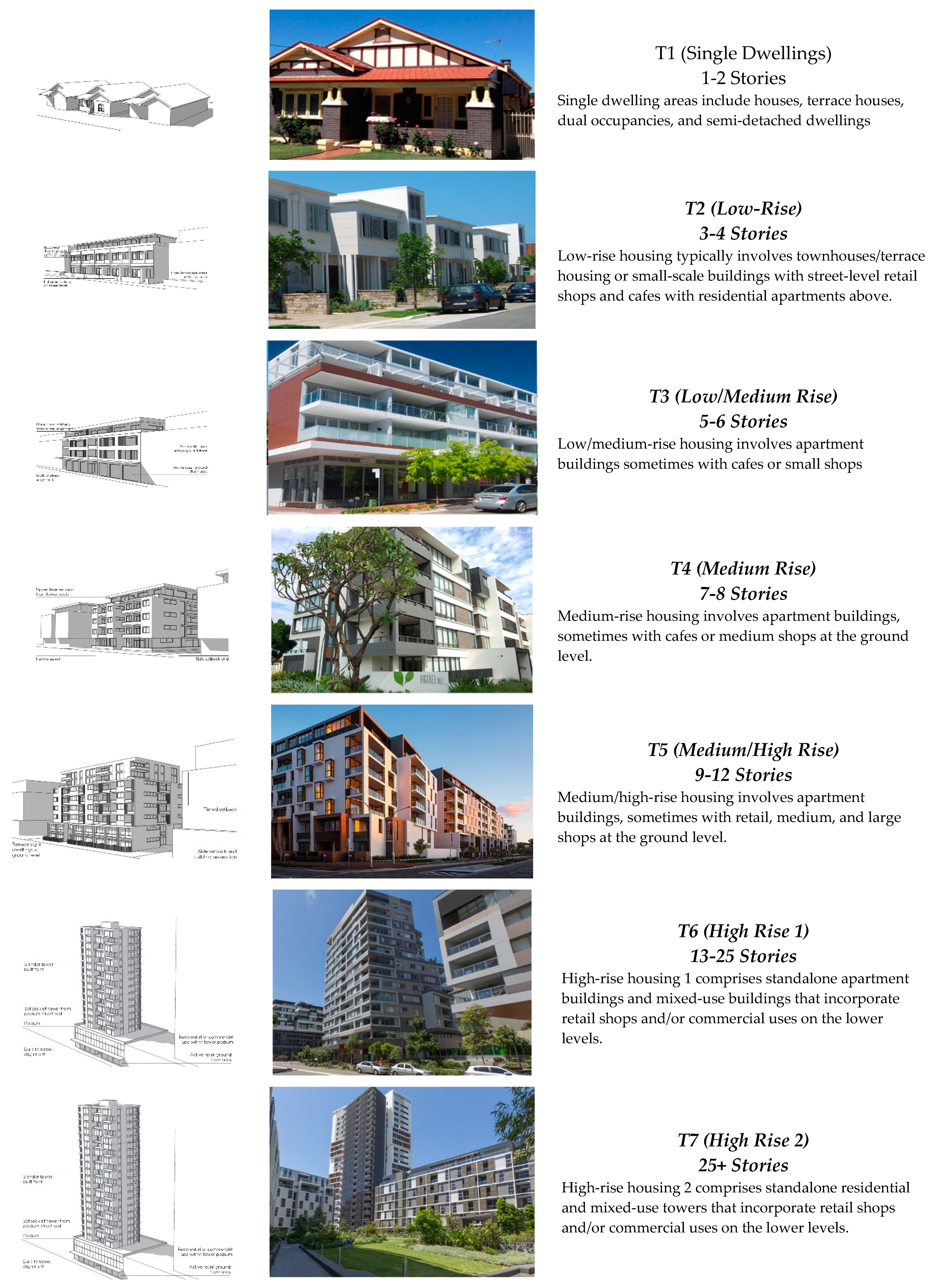
2.3. Urban Classification Method
3. Modelling Method
- Typically, the horizontal resolution is between 0.5 and 5 m;
- Typically, the time frame is between 24 and 48 h;
- Typically, the time step is between 1 and 5 s.
3.1. Resolution Settings
3.2. Simple Forcing
3.3. Comfort Evaluation
4. Simulation Results
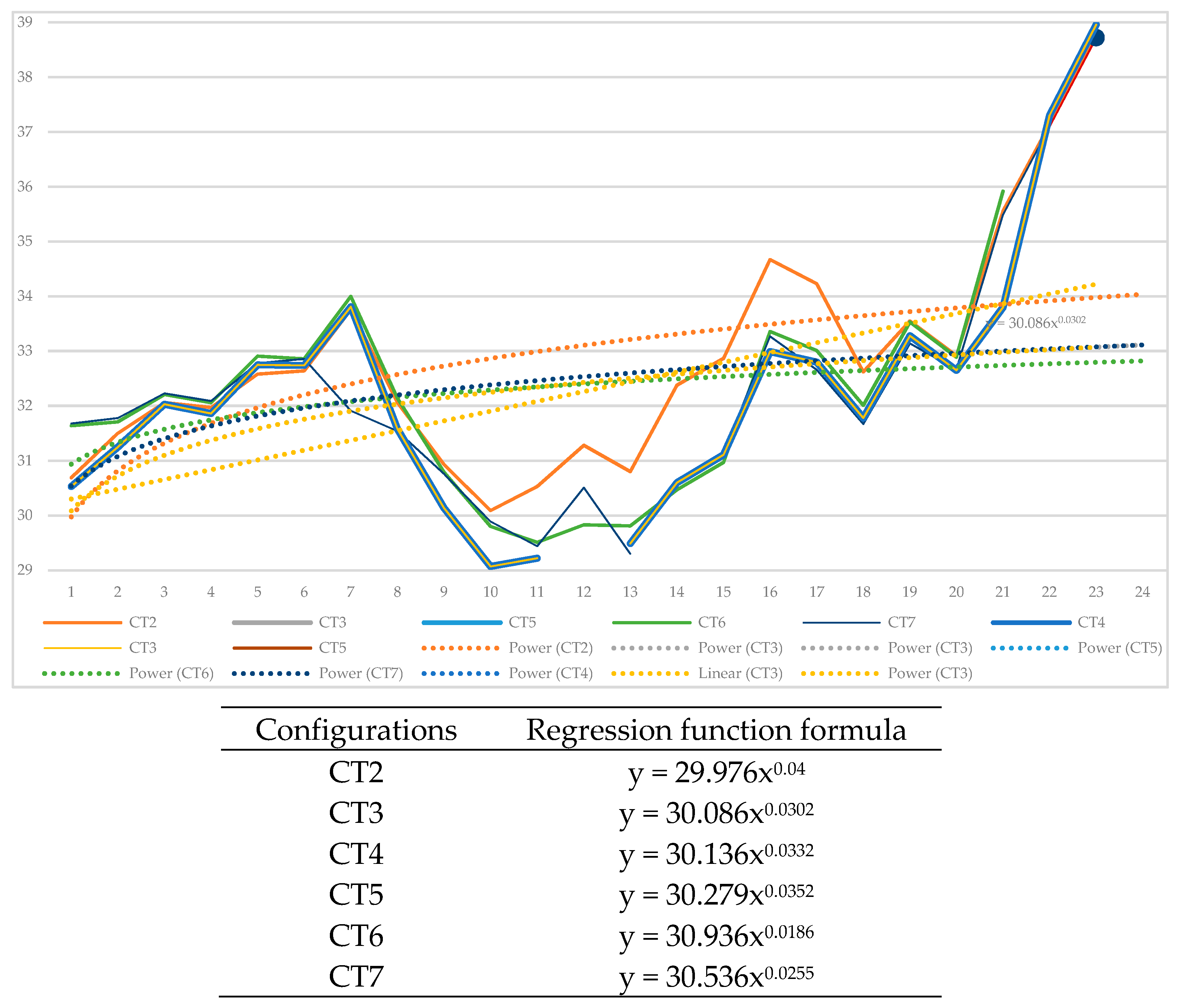
4.1. Compact Arrangements and Heat Island Effect
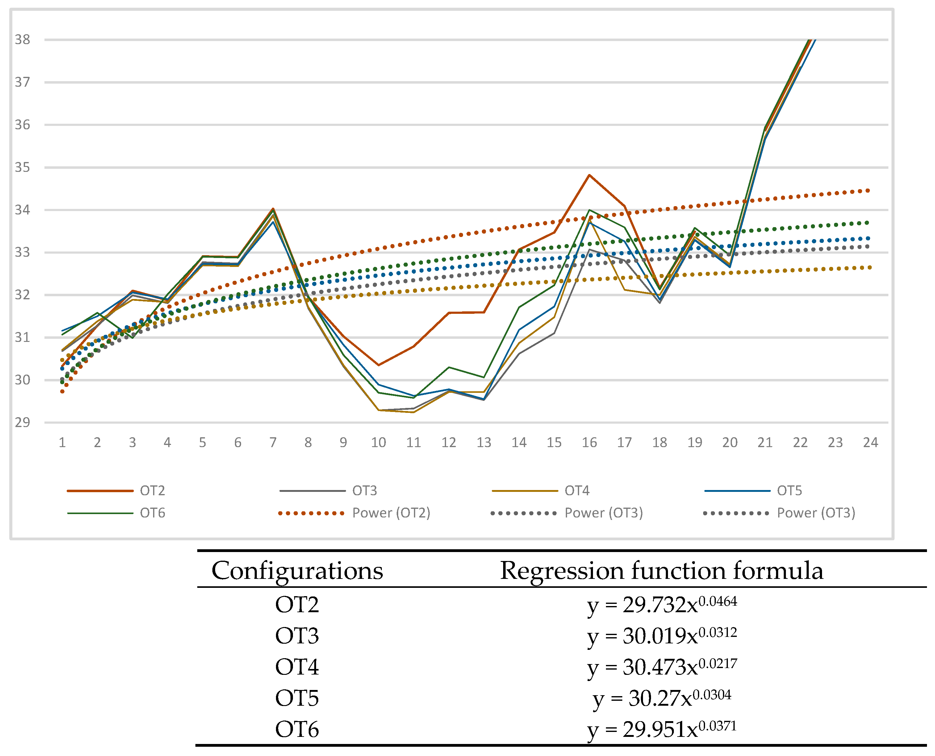
4.2. Open Type Arrangements and Heat Island Effect
5. Analysis of Results and Discussion
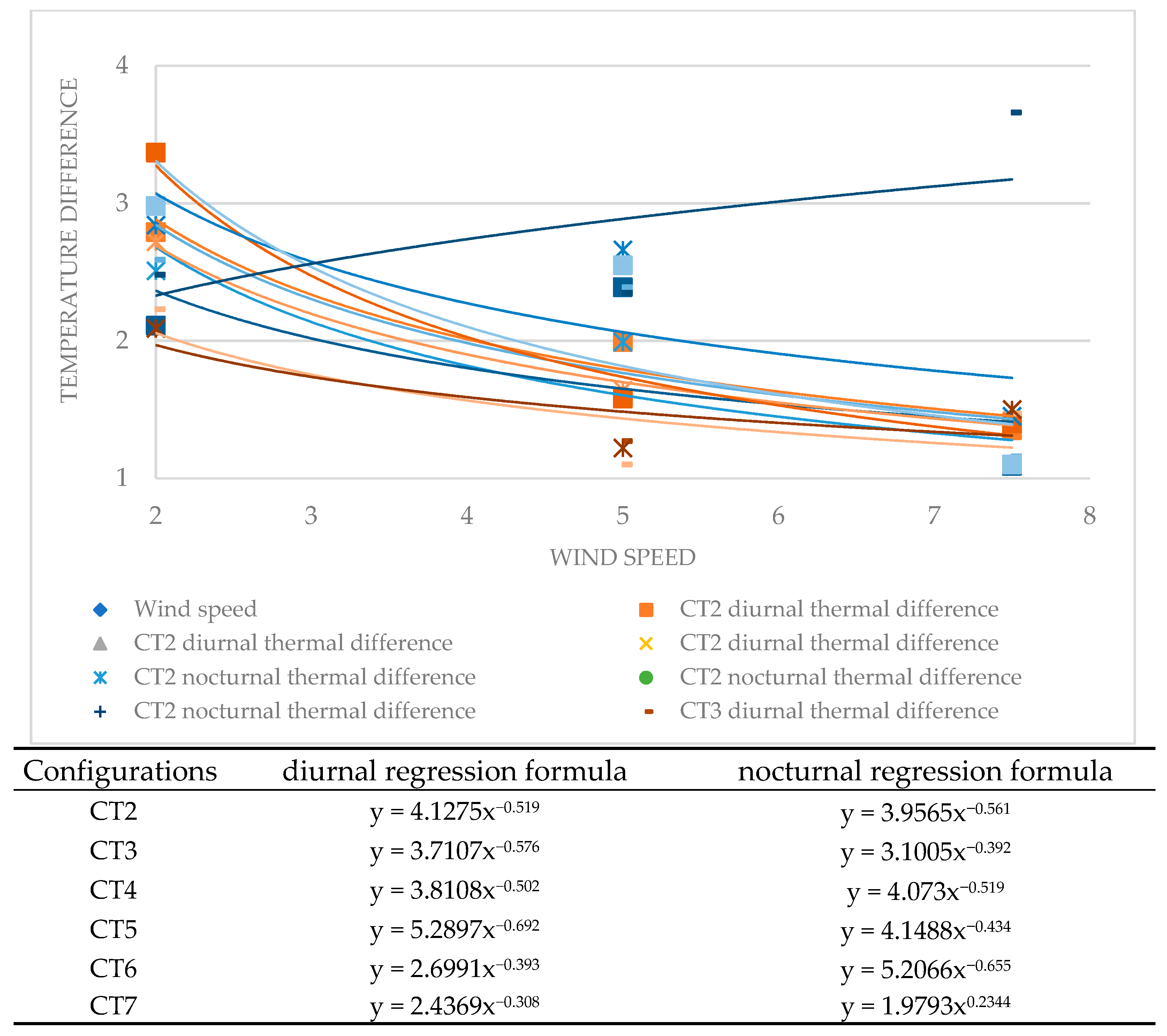
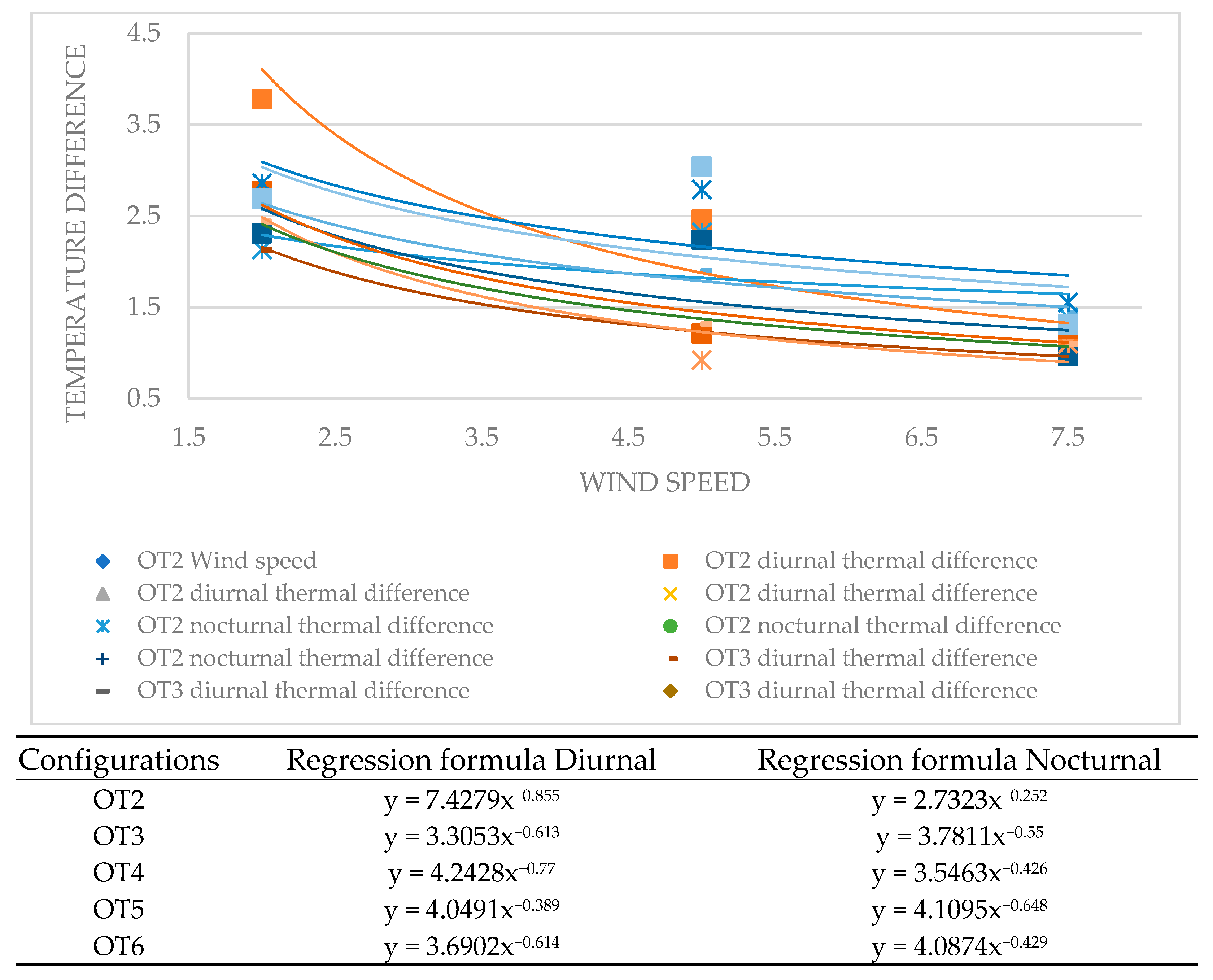
5.1. Layouts Temperature Difference and Wind Speed
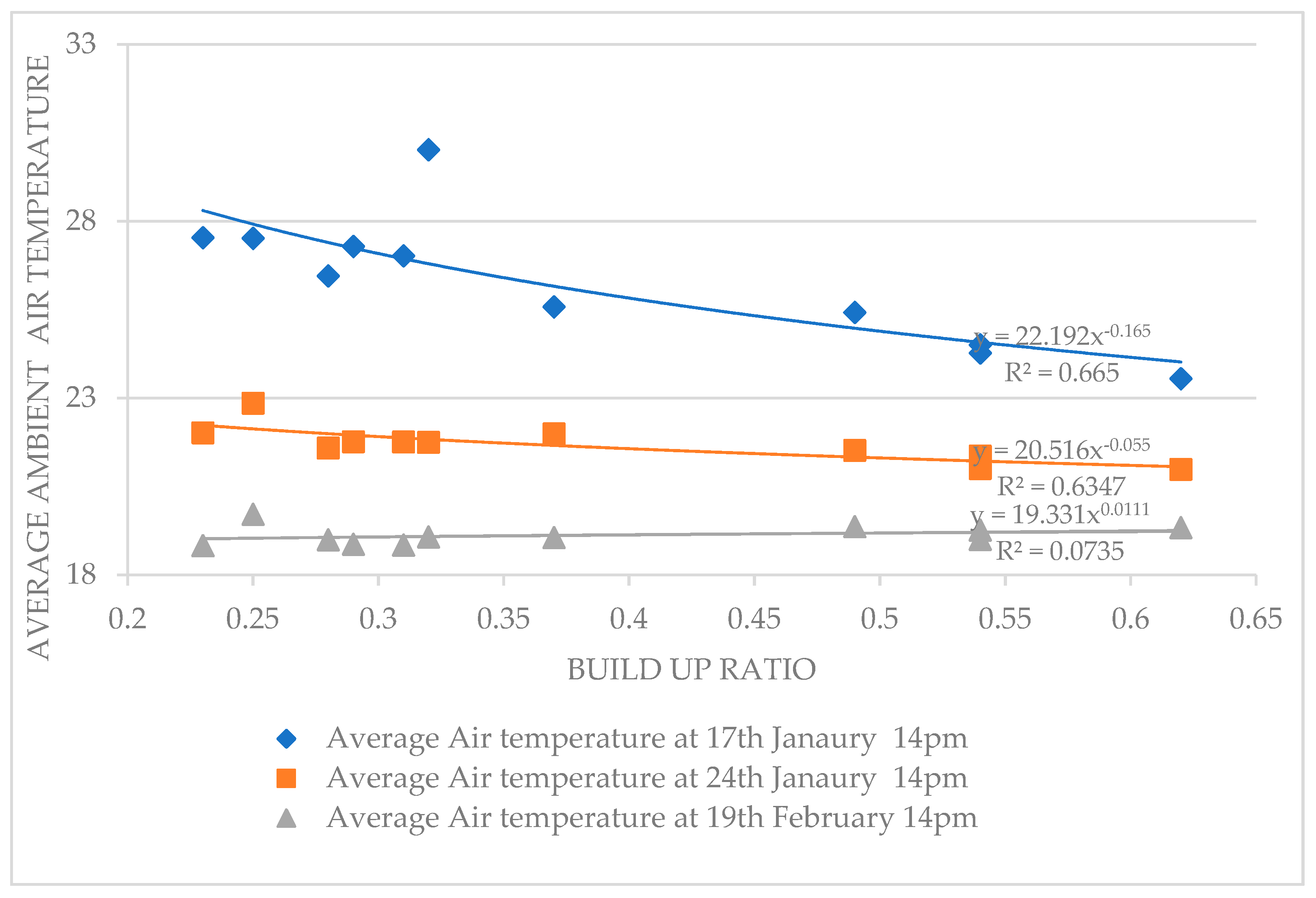
5.2. Built-Up Ratio and Average Ambient Temperature
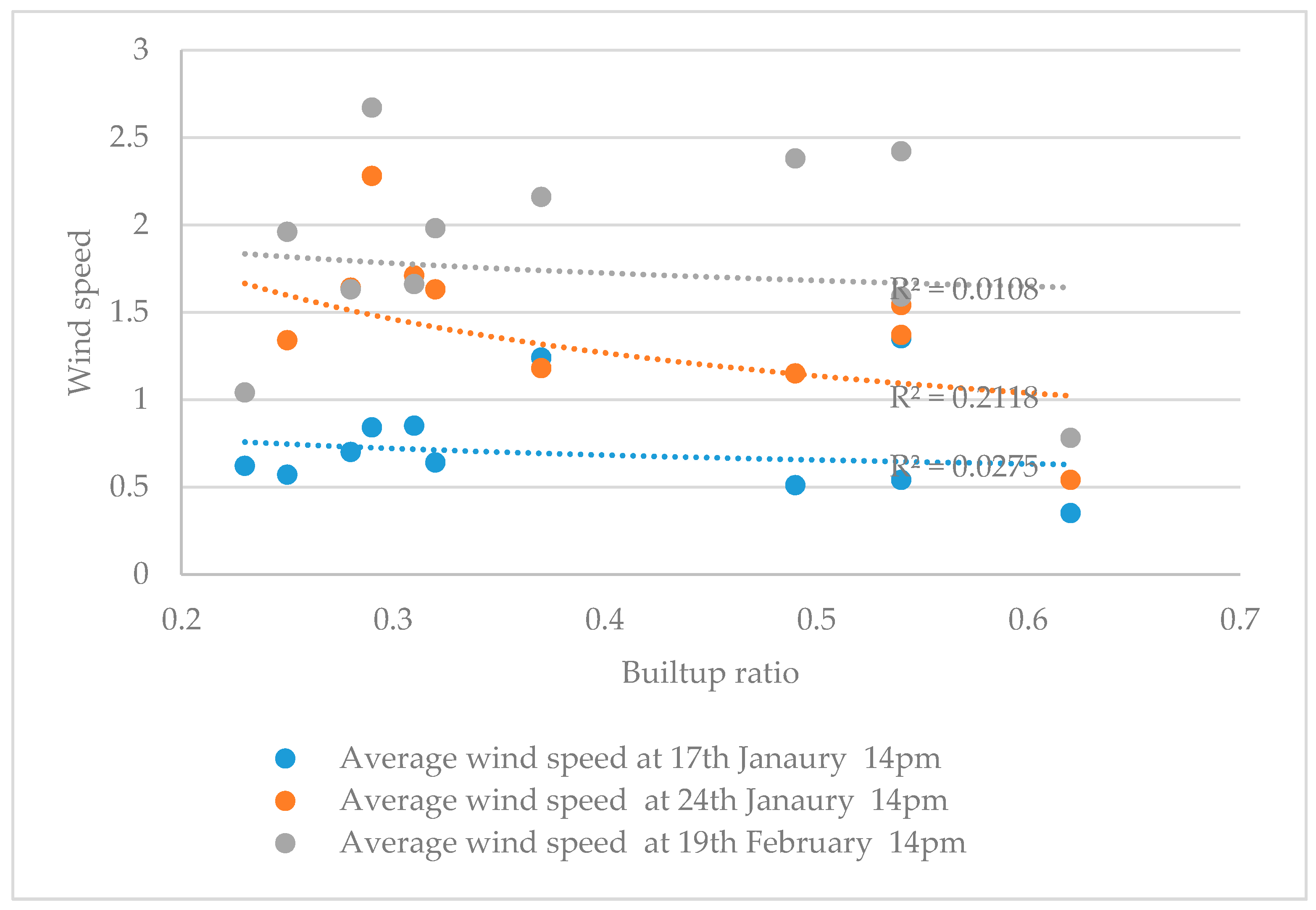
5.3. Built-Up Ratio and Average Wind Speed
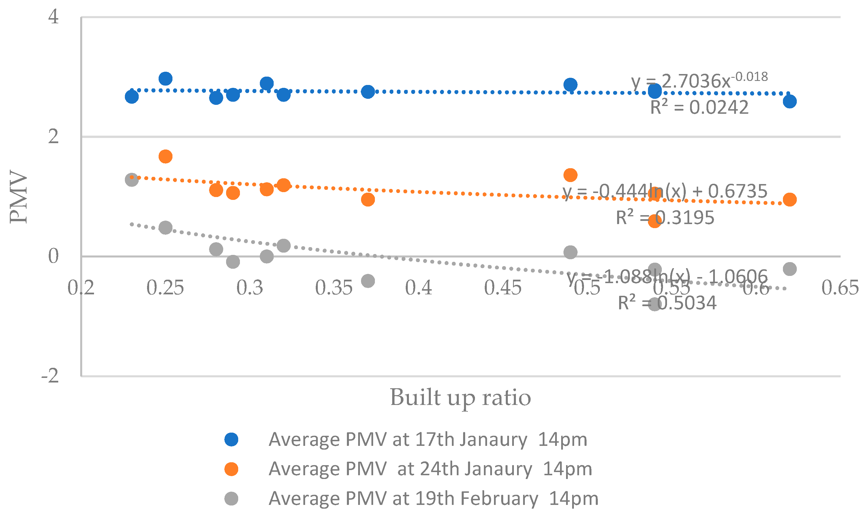
5.4. Built-Up Ratio and Average PMV
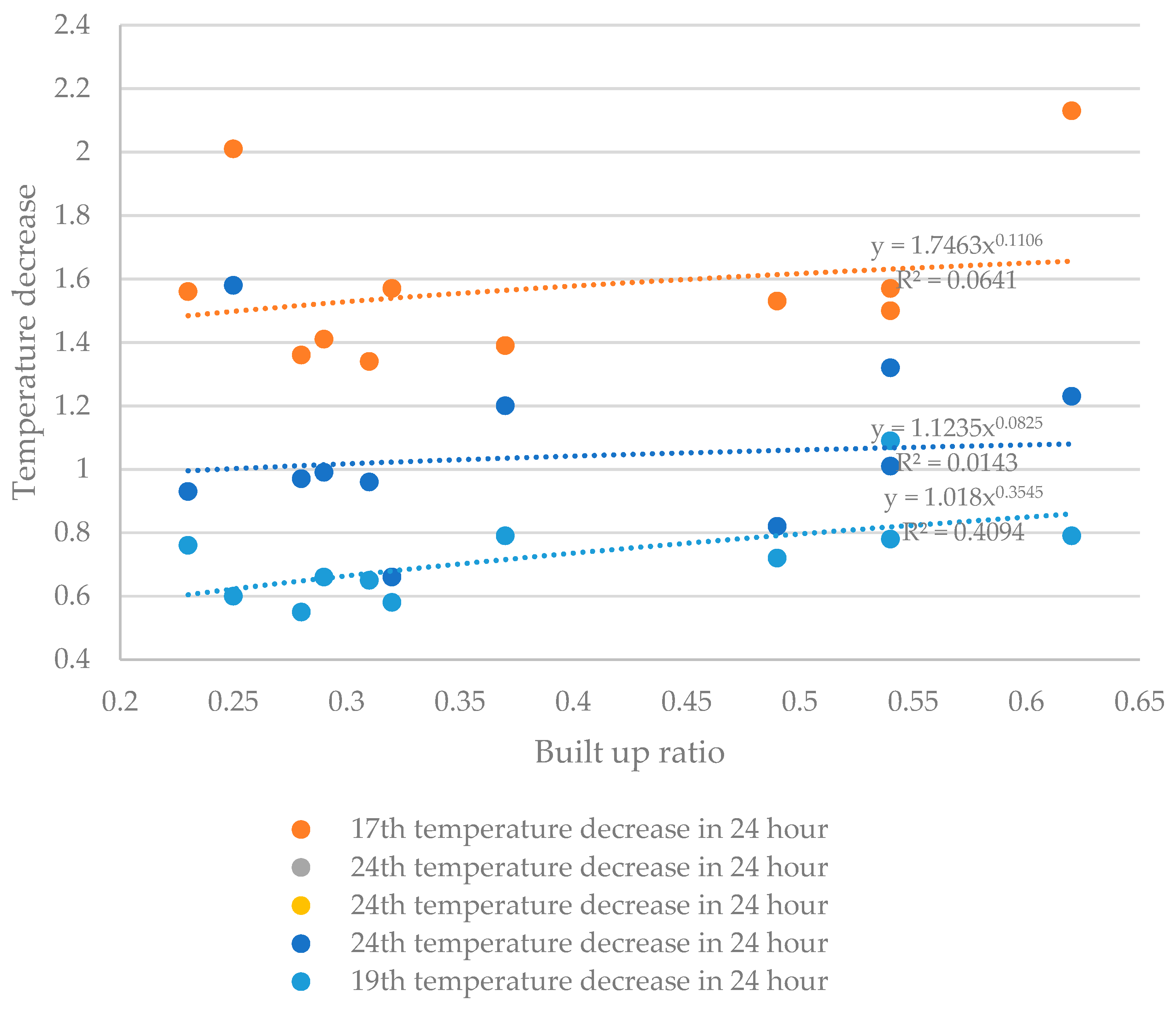
5.5. Built-Up Ratio and Average Hourly Temperature Decrease
6. Conclusions
Author Contributions
Funding
Data Availability Statement
Conflicts of Interest
Appendix A
Appendix A.1. Technical Characteristics of the Field Work Measurement Equipment

| Parameter | Value |
|---|---|
| ISO classification (ISO 9060: 1990) | second class pyranometer |
| Response time (95 %) | 18 s |
| Zero offset a (response to 200 W/m2 net thermal radiation | <±15 W/m2 unventilated |
| Non-linearity | <±1% (100 to 1000 W/m2) |
| Directional response | < ± 25 W/m2 |
| Spectral selectivity | <±5% (0.35 to 1.5 × 10⁻⁶ m) |
| Temperature response | <±3% (−10 to 40 °C) |
| Quantity Parameters Value | Quantity Parameters Value | Quantity Parameters Value |
|---|---|---|
| Wind | Wind Speed Range | 0–60 m/s |
| Wind Speed Accuracy | ±2% @12 m/s | |
| Wind Speed Resolution | 0.01 m/s | |
| Wind Direction Range | 0 to 359°—No dead band | |
| Wind Direction Accuracy | ±3° @12 m/s | |
| Wind Direction Resolution | 1° | |
| Temperature | Air Temperature | Pt100 1/3 Class B |
| Range | −50 °C to +100 °C | |
| Accuracy | ±0.1 °C | |
| Resolution | 0.1 °C | |
| Barometric pressure | Range | 600–1100 hPa |
| Accuracy | ±0.5 hPa |
Appendix A.2. Summary of Heat Island Effect in Compact Type Series
| 17 January | 24 January | 19 February | ||
| CT2 | Ambient temperature diurnal |  4 p.m. |  1 p.m. |  7 a.m. |
| Ambient temperature nocturnal |  23 p.m. |  1 a.m. |  5 a.m. | |
| Wind |  |  |  | |
| CT4 | Ambient air temperature diurnal |  16 p.m. |  13 p.m. |  7 a.m. |
| Ambient air temperature nocturnal |  23 p.m. |  1 a.m. |  5 a.m. | |
| Wind |  |  |  | |
| CT6 | Ambient air temperature diurnal |  16 p.m. |  1 p.m. |  7 a.m. |
| Ambient air temperature nocturnal |  11 p.m. |  1 a.m. |  5 a.m. | |
| Wind |  |  |  |
Appendix A.3. Summary of Heat Island Effect in Open Type Series
| 17 January | 24 January | 19 February | ||
| OT2 | Ambient air temperature diurnal |  16 p.m. |  13 p.m. |  7 a.m. |
| Ambient air temperature nocturnal |  23 p.m. |  1 a.m. |  5 a.m. | |
| Wind |  |  |  | |
| OT3 | Ambient air temperature diurnal |  4 p.m. |  1 p.m. |  7 a.m. |
| Ambient air temperature nocturnal |  11 p.m. |  1 a.m. |  5 a.m. | |
| Wind |  |  |  | |
| OT5 | Ambient air temperature diurnal |  16 p.m. |  13 p.m. |  7 a.m. |
| Ambient air temperature nocturnal |  23 p.m. |  1 a.m. |  5 a.m. | |
| Wind |  |  |  |
References
- Santamouris, M.; Haddad, S.; Saliari, M.; Vasilakopoulou, K.; Synnefa, A.; Paolini, R.; Ulpiani, G.; Garshasbi, S.; Fiorito, F. On the energy impact of urban heat island in Sydney: Climate and energy potential of mitigation technologies. Energy Build. 2018, 166, 154–164. [Google Scholar] [CrossRef]
- Oke, T.R. Boundary Layer Climates; Routledge: London, UK, 2002. [Google Scholar]
- Santamouris, M.; Haddad, S.; Fiorito, F.; Osmond, P.; Ding, L.; Prasad, D.; Zhai, X.; Wang, R. Urban Heat Island and Overheating Characteristics in Sydney, Australia. An Analysis of Multiyear Measurements. Sustainability 2017, 9, 712. [Google Scholar] [CrossRef]
- Oke, T.R. The energetic basis of the urban heat island. Q. J. R. Meteorol. Soc. 1982, 108, 1–24. [Google Scholar] [CrossRef]
- Khalili, S.M.; Jolai, F.; Torabi, S.A. Integrated production–distribution planning in two-echelon systems: A resilience view. Int. J. Prod. Res. 2017, 55, 1040–1064. [Google Scholar] [CrossRef]
- Cleugh, H.; Cleugh, H.; Smith, M.S.; Battaglia, M.; Grah a.m., P. Climate Change: Science and Solutions for Australia; CSIRO: Canberra, Australia, 2006. [Google Scholar]
- Mirmozaffari, M.; Yazdani, R.; Shadk a.m., E.; Khalili, S.M.; Tavassoli, L.S.; Boskabadi, A. A novel hybrid parametric and non-parametric optimisation model for average technical efficiency assessment in public hospitals during and post-COVID-19 pandemic. Bioengineering 2021, 9, 7. [Google Scholar] [CrossRef] [PubMed]
- Pearce, K.; Holper, P.; Hopkins, M.; Bouma, W.; Whetton, P.; Hennessy, K.; Power, S. Climate Change in Australia; CSIRO: Canberra, Australia, 2007. [Google Scholar]
- Wang, X.; Chen, D.; Ren, Z. Assessment of climate change impact on residential building heating and cooling energy requirement in Australia. Build. Environ. 2010, 45, 1663–1682. [Google Scholar] [CrossRef]
- Rizwan, A.M.; Dennis, L.Y.; Chunho, L. A review on the generation, determination and mitigation of Urban Heat Island. J. Environ. Sci. 2008, 20, 120–128. [Google Scholar] [CrossRef] [PubMed]
- Asfour, O. Prediction of wind environment in different grouping patterns of housing blocks. Energy Build. 2010, 42, 2061–2069. [Google Scholar] [CrossRef]
- Sibevei, A.; Azar, A.; Zandieh, M.; Khalili, S.M.; Yazdani, M. Developing a Risk Reduction Support System for Health System in Iran: A Case Study in Blood Supply Chain Management. Int. J. Environ. Res. Public Health 2022, 19, 2139. [Google Scholar] [CrossRef]
- Che-Ani, A.; Shahmohamadi, P.; Sairi, A.; Mohd-Nor, M.; Zain, M.; Surat, M. Mitigating the urban heat island effect: Some points without altering existing city planning. Eur. J. Sci. Res. 2009, 35, 204–216. [Google Scholar]
- Santamouris, M.; Papanikolaou, N.; Livada, I.; Koronakis, I.; Georgakis, C.; Argiriou, A.; Assimakopoulos, D. On the impact of urban climate on the energy consumption of buildings. Sol. Energy 2001, 70, 201–216. [Google Scholar] [CrossRef]
- Steemers, K.; Baker, N.; Crowther, D.; Dubiel, J.; Nikolopoulou, M. Radiation absorption and urban texture. Build. Res. Inf. 1998, 26, 103–112. [Google Scholar] [CrossRef]
- Morris, C.; Simmonds, I.; Plummer, N. Quantification of the influences of wind and cloud on the nocturnal urban heat island of a large city. J. Appl. Meteorol. Climatol. 2001, 40, 169–182. [Google Scholar] [CrossRef]
- Shashua-Bar, L.; Tzamir, Y.; Hoffman, M.E. Thermal effects of building geometry and spacing on the urban canopy layer microclimate in a hot-humid climate in summer. Int. J. Clim. 2004, 24, 1729–1742. [Google Scholar] [CrossRef]
- Thapar, H.; Yannas, S. 491: Microclimate and Urban Form in Dubai. In Proceedings of the 25th Conference on Passive and Low Energy Architecture, Dubai, United Arab Emirates, 22–24 October 2008. [Google Scholar]
- Bourbia, F.; Boucheriba, F. Impact of street design on urban microclimate for semi arid climate (Constantine). Renew. Energy 2010, 35, 343–347. [Google Scholar] [CrossRef]
- Erell, E.; Pearlmutter, D.; Williamson, T. Urban Microclimate: Designing the Spaces between Buildings; Routledge: London, UK, 2012. [Google Scholar]
- Heshmat Mohajer, H.R.; Ding, L.; Santamouris, M. Developing Heat Mitigation Strategies in the Urban Environment of Sydney, Australia. Buildings 2022, 12, 903. [Google Scholar] [CrossRef]
- Golany, G.S. Urban design morphology and thermal performance. Atmos. Environ. 1996, 30, 455–465. [Google Scholar] [CrossRef]
- Yang, Y.; Jin, X.-Y.; Yang, L.-G.; Jin, H.; Xue, M.; Zheng, Z.-Y. Numerical Simulation Research on Pedestrian Wind Environment and Optimization Design of High-Rise Buildings. Build. Sci. 2011, 27, 4–8. [Google Scholar]
- Kolokotsa, D.; Lilli, K.; Gobakis, K.; Mavrigiannaki, A.; Haddad, S.; Garshasbi, S.; Mohajer, H.R.H.; Paolini, R.; Vasilakopoulou, K.; Bartesaghi, C.; et al. Analyzing the Impact of Urban Planning and Building Typologies in Urban Heat Island Mitigation. Buildings 2022, 12, 537. [Google Scholar] [CrossRef]
- Ali-Toudert, F.; Mayer, H. Numerical study on the effects of aspect ratio and orientation of an urban street canyon on outdoor thermal comfort in hot and dry climate. Build. Environ. 2006, 41, 94–108. [Google Scholar] [CrossRef]
- Australian Bureau of Statistics. Australian Statistical Geography Standard (ASGS); Australian Bureau of Statistics: Canberra, Australia, 2011.
- De Dear, R.; Kim, J.; Parkinson, T. Residential adaptive comfort in a humid subtropical climate—Sydney Australia. Energy Build. 2018, 158, 1296–1305. [Google Scholar] [CrossRef]
- Fahmy, M.; Sharples, S. On the development of an urban passive thermal comfort system in Cairo, Egypt. Build. Environ. 2009, 44, 1907–1916. [Google Scholar] [CrossRef]
- Krüger, E.L.; Minella, F.O.; Rasia, F. Impact of urban geometry on outdoor thermal comfort and air quality from field measurements in Curitiba, Brazil. Build. Environ. 2011, 46, 621–634. [Google Scholar] [CrossRef]
- Bruse, M. Modelling and strategies for improved urban climates. In Proceedings of the Proceedings International Conference on Urban Climatology & International Congress of Biometeorology, Sydney, Australia, 8–12 November 1999. [Google Scholar]
- Morakinyo, T.E.; Lau, K.K.-L.; Ren, C.; Ng, E. Environment. Performance of Hong Kong’s common trees species for outdoor temperature regulation, thermal comfort and energy saving. Build. Environ. 2018, 137, 157–170. [Google Scholar] [CrossRef]
- Stelling, G.; Zijlema, M. An accurate and efficient finite-difference algorithm for non-hydrostatic free-surface flow with application to wave propagation. Int. J. Numer. Methods Fluids 2003, 43, 1–23. [Google Scholar] [CrossRef]
- Acero, J.A.; Arrizabalaga, J. Evaluating the performance of ENVI-met model in diurnal cycles for different meteorological conditions. Arch. Meteorol. Geophys. Bioclimatol. Ser. B 2016, 131, 455–469. [Google Scholar] [CrossRef]


| Designated Tracks | Thermal Camera | Portable Station—Net Radiometer | |
|---|---|---|---|
| First Track |  |  |  |
| Second Track |  |  |  |
| A | B | C | D | E | F | |||||||||||||||||||||
|---|---|---|---|---|---|---|---|---|---|---|---|---|---|---|---|---|---|---|---|---|---|---|---|---|---|---|
| Point | −33.894004 | 151.254918 | −33.89316 | 151.254928 | −33.892689 | 151.251963 | −33.894097 | 151.251484 | −33.893156 | 151.25493 | −33.892689 | 151.251963 | ||||||||||||||
| Record Time | 10:45 | 11:45 | 16:38 | 16:38 | 11:53 | 10:59 | 12.02 | 11.07 | 12:10 | 11:20 | 12:17 | 10:59 | 13:01 | |||||||||||||
| Ambient Temperature | 18 | 18.9 | 17.5 | 17.5 | 19.4 | 18.3 | 19.2 | 17.9 | 19.4 | 18.2 | 19.5 | 18.3 | 19.5 | |||||||||||||
| Surface Temperature | 27.1 | 16.3 | 27.7 | 13.4 | 25.2 | 20.1 | 38 | 15 | 27.1 | 20.2 | 34.5 | 14.1 | 39.7 | 26.7 | 37.5 | 27.4 | 27.4 | 15.1 | 33.1 | 15 | 44 | 17 | 34.5 | 14 | 24.6 | 14.6 |
| Wind Speed (m/s) | 1 | 0.7 | 1.1 | 1.1 | 1.4 | 0.5 | 1.2 | 0.1 | 0.1 | 0.1 | 0.7 | 0.5 | 0.5 | |||||||||||||
| Wind Direction | 215 | 150 | 207 | 207 | 278 | 317 | 2 | 39 | 9 | 39 | 27 | 317 | 239 | |||||||||||||
| Pavement Type | LCP | DCP | LCP | LCP | DCP | LCP | ||||||||||||||||||||
| Open Arrangements | |||||
|---|---|---|---|---|---|
| Type | OT2: Open Low Rise | OT3: Open Low/Medium Rise | OT4: Open Medium Rise | OT5: Open Medium/High Rise | OT6: Open High Rise 1 |
| Figure |  |  |  |  |  |
| 2D Aerial View |  |  |  |  |  |
| Google earth point | 33°53′31.80″ S 151°13′55.72″ E | 33°53′30.5″ S 151°15′41.0″ E | 33°50′04.8″ S 151°12′36.6″ E | 33°53′17.7″ S 151°12′37.4″ E | 33°52′57.4″ S 151°12′31.8″ E |
| Site dimension | 78.5 × 120 | 82.5 × 124.5 | 77 × 115.5 | 168.5 × 211 | 199 × 183 |
| Address | 24 Mitchell St, Centennial Park NSW 2021, Australia | Penkivil St, Bondi NSW 2026, Australia | 199 Walker St, North Sydney NSW 2060, Australia | Methadone clinics, Lee St and, Little Regent St, Chippendale NSW 2008 | Surry Hills NSW 2010, Australia |
| Compact Arrangements | |||||
|---|---|---|---|---|---|
| Type | CT2: Open Low Rise | CT4: Open Medium Rise | CT5: Open Medium/High Rise | CT6: Open High Rise 1 | CT7: Open High Rise 2 |
| Figure |  |  |  |  |  |
| 2D Aerial View |  |  |  |  |  |
| Google earth point | 33°53′32.58″ S 151°14′40.03″ E | 33°53′26.72″ S 151°15′43.19″ E | 33°52′42.8″ S 151°12′45.2″ E | 33°52′43.86″ S 151°12′28.31″ E | 33°52′1.44″ S 151°12′40.65″ E |
| Site dimension | 72 × 105 | 117 × 167 | 84 × 111 | 131 × 176 | 156 × 143 |
| Address | 47 Denison St, Bondi Junction NSW 2022, Australia | c7/99 Jones St, Ultimo NSW 2007, Australia | 162–166 Goulburn St, Surry Hills NSW 2010, Australia | 311–315 Castlereagh St, Haymarket NSW 2000, Australia | 126–146 Phillip St, Sydney NSW 2000, Australia |
| Thermal and Humidity Profile | A | B | C | D | E | F |
|---|---|---|---|---|---|---|
 17 January | 2 | 90 | 50 | 0.01 | 7 | 26.35–40.17 |
 24 January | 5 | 0 | 50 | 0.011 | 7 | 19.95–38.27 |
 19 February | 7.5 | 135 | 50 | 0.01 | 7 | 14.85–20.85 |
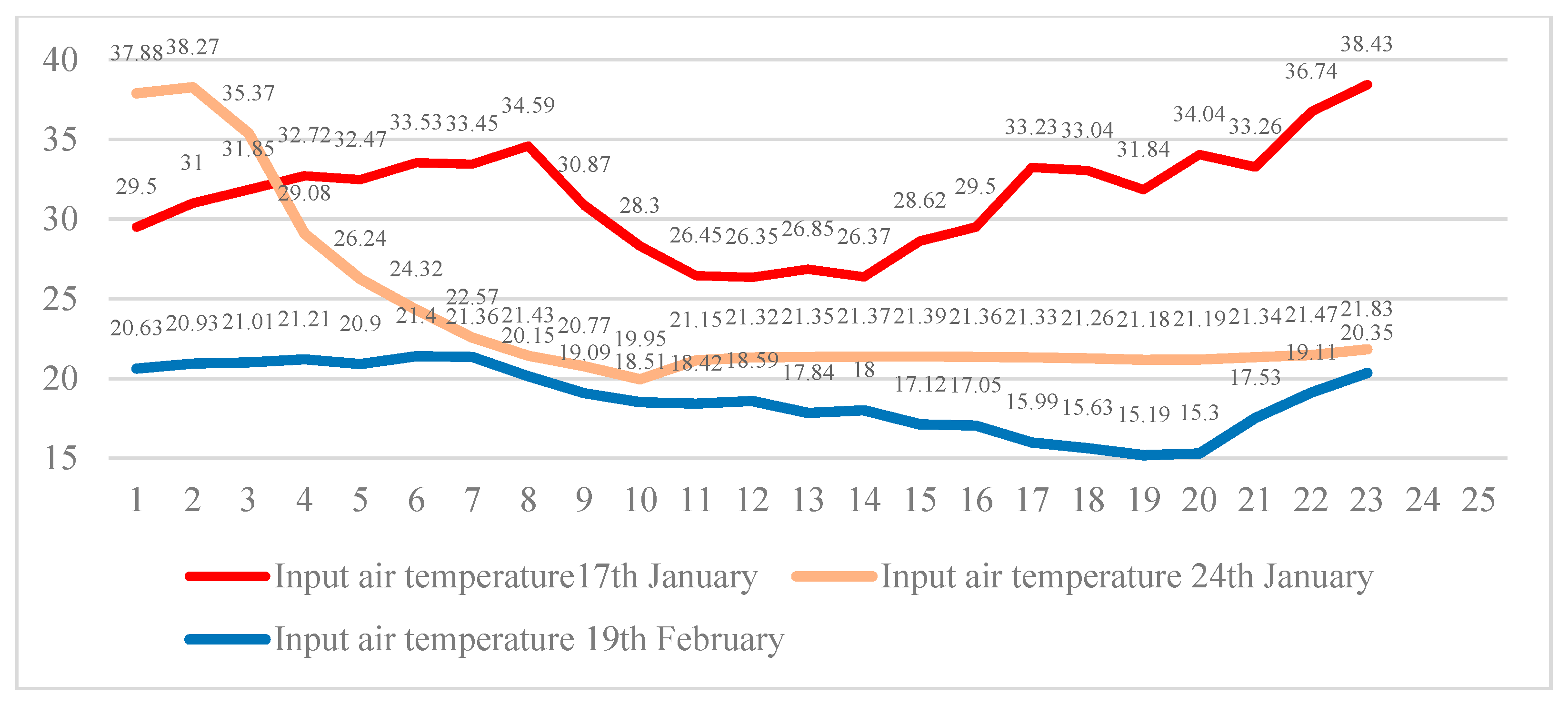
| 1 | 2 | 3 | 4 | 5 | 6 | 7 | 8 | 9 | 10 | 11 | 12 | |
| 17 January | 29.5 | 31 | 31.85 | 32.72 | 32.47 | 33.53 | 33.45 | 34.59 | 30.87 | 28.3 | 26.45 | 26.35 |
| 24 January | 37.88 | 38.27 | 35.37 | 29.08 | 26.24 | 24.32 | 22.57 | 21.43 | 20.77 | 19.95 | 21.15 | 21.32 |
| 19 February | 20.63 | 20.93 | 21.01 | 21.21 | 20.9 | 21.4 | 21.36 | 20.15 | 19.09 | 18.51 | 18.42 | 18.59 |
| 13 | 14 | 15 | 16 | 17 | 18 | 19 | 20 | 21 | 22 | 23 | ||
| 17 January | 26.85 | 26.37 | 28.62 | 29.5 | 33.23 | 33.04 | 31.84 | 34.04 | 33.26 | 36.74 | 38.43 | |
| 24 January | 21.35 | 21.37 | 21.39 | 21.36 | 21.33 | 21.26 | 21.18 | 21.19 | 21.34 | 21.47 | 21.83 | |
| 19 February | 17.84 | 18 | 17.12 | 17.05 | 15.99 | 15.63 | 15.19 | 15.3 | 17.53 | 19.11 | 20.35 |
| Precinct | Simulation Period | Max Heat Intensity | Temperature Decrease | Canyon Properties | Ventilation | ||||||
|---|---|---|---|---|---|---|---|---|---|---|---|
| T Max | T Min | Wind Speed | Diurnal | Nocturnal | Total | Average | Aspect Ratio | Orientation | |||
| CT2 | 17 January | 34.67 °C | 28.17 °C | 1.28 m/s | 6.01 °C | 1.71 °C | 36.74 °C | 1.530 °C | 0.45 | N-S | Blocked |
| 24 January | 23.54 °C | 20.70 °C | 4.05 m/s | 2.33 °C | 0.35 °C | 19.88 °C | 0.828 °C | 0.41 | E-W | Moderate | |
| 19 February | 20.51 °C | 14.68 °C | 5.59 m/s | 2.01 °C | 0.53 °C | 17.5 °C | 0.729 °C | 0.43 | N-S | Uniform | |
| CT3 | 17 January | 38.96 °C | 27.3 °C | 3.082 m/s | 4.23 °C | 1.44 °C | 32.36 °C | 1.348 °C | 0.79 | N-S | Uniform |
| 24 January | 28.91 °C | 20.5 °C | 4.63 m/s | 2.05 °C | 0.45 °C | 23.05 °C | 0.96 °C | 054 | E-W | Moderate | |
| 19 February | 20.17 °C | 14.55 °C | 6.65 m/s | 1.1 °C | 0.41 °C | 15.71 °C | 0.654 °C | 0.43 | N-S | large masking | |
| CT4 | 17 January | 38.99 °C | 27.4 °C | 3.89 m/s | 4.73 °C | 2.74 °C | 37.73 °C | 1.572 °C | 1.062 | N-S | blocked |
| 24 January | 29.64 °C | 20.52 °C | 5.74 m/s | 2.01 °C | 0.64 °C | 24.24 °C | 1.01 °C | 0.64 | N-S | masking area | |
| 19 February | 20.26 °C | 14.75 °C | 9.19 m/s | 1.16 °C | 1.42 °C | 18.78 °C | 0.782 °C | 1.1 | N-S | moderate | |
| CT5 | 17 January | 38.96 °C | 27.3 °C | 3.082 m/s | 4.73 °C | 2.74 °C | 48.89 °C | 2.037 °C | 3.1 | E-W | Blocked |
| 24 January | 29.75 °C | 20.86 °C | 4.23 m/s | 2.52 °C | 0.63 °C | 24.96 °C | 1.04 °C | 3.1 | E-W | Masking area | |
| 19 February | 20.17 °C | 14.55 °C | 9.15 m/s | 1.38 °C | 1.01 °C | 19.11 °C | 0.796 °C | 2.4 | N-S | Blocked | |
| CT6 | 17 January | 39.18 °C | 27.6 °C | 5.5 m/s | 4.16 °C | 2.23 °C | 33.56 °C | 1.393 °C | 7.5 | N-S | uniform |
| 24 January | 20.8 °C | 29.75 °C | 6.07 m/s | 2.01 °C | 0.64 °C | 20.34 °C | 0.847 °C | 4.76 | E-W | blocked | |
| 19 February | 20.3 °C | 15.3 °C | 12.47 m/s | 1.41 °C | 1.21 °C | 19.01 °C | 0.792 °C | 3–5.2 | N-S | uniform | |
| CT7 | 17 January | 38.72 °C | 27.4 °C | 5.5 m/s | 4.16 °C | 2.23 °C | 36.14 °C | 1.505 °C | 4.32 | N-S | moderate |
| 24 January | 29.75 °C | 20.6 °C | 6.02 m/s | 2.01 °C | 0.64 °C | 21.56 °C | 0.898 °C | 4.2–4.32 | E-W | blocked | |
| 19 February | 20.23 °C | 14.63 °C | 12.55 m/s | 1.1 °C | 1.39 °C | 26.16 °C | 1.09 °C | 4.2–4.32 | E-W | moderate | |
| Compact Types | |
|---|---|
| Diurnal | Nocturnal |
 |  |
| 17 January CT2 | |
 |  |
| 17 January CT4 | |
 |  |
| 17 January CT7 | |
| CT2 | CT3 |
 |  |
| CT4 | CT5 |
 |  |
| CT6 | CT7 |
 |  |
| CT2 | CT4 |
 |  |
| CT5 | CT6 |
 |  |
| Precinct | Simulation Period | Ambient Temperature in the Canyon | Max Heat Intensity | Temperature Decrease | Canyon Properties | Ventilation | |||||
|---|---|---|---|---|---|---|---|---|---|---|---|
| Max | Min | Wind Speed | Diurnal | Nocturnal | Total | Average | Aspect Ratio | Orientation | |||
| OT2 | 17 January | 39.14 °C | 27.2 °C | 2.016 m/s | 6.7 °C | 2.61 °C | 51.31 °C | 2.137 °C | 0.41 | E-W | uniform |
| 24 January | 28.24 °C | 19.81 °C | 3.52 m/s | 3.45 °C | 0.43 °C | 38.15 °C | 1.589 °C | 0.45 | N-S | uniform | |
| 19 February | 20.16 °C | 14.2 °C | 4.37 m/s | 1.1 °C | 1.39 °C | 14.48 °C | 0.603 °C | 0.45 | N-S | moderate | |
| OT3 | 17 January | 38.96 °C | 27.2 °C | 2.89 m/s | 4.25 °C | 2.4 °C | 32.67 °C | 1.361 °C | 0.79 | N-S | uniform |
| 24 January | 30.24 °C | 20 °C | 4.92 m/s | 1.29 °C | 2.24 °C | 23.39 °C | 0.974 °C | 0.79 | N-S | moderate | |
| 19 February | 20.13 °C | 14.62 °C | 6.56 m/s | 1.13 °C | 0.32 °C | 13.22 °C | 0.550 °C | 0.79 | N-S | blocked | |
| OT4 | 17 January | 38.99 °C | 27.4 °C | 2.22 m/s | 5.09 °C | 2.47 °C | 37.73 °C | 1.572 °C | 0.12 | N-S | uniform |
| 24 January | 29.46 °C | 20.94 °C | 4.96 m/s | 1.74 °C | 0.66 °C | 15.98 °C | 0.665 °C | 0.34 | N-S | uniform | |
| 19 February | 20.16 °C | 14.55 °C | 5.85 m/s | 1.31 °C | 0.69 °C | 14.06 °C | 0.585 °C | 0.12 | N-S | moderate | |
| OT5 | 17 January | 38.93 °C | 27.12 °C | 2.07 m/s | 4.81 °C | 2.471 °C | 37.47 °C | 1.561 °C | 1.02 | E-W | blocked |
| 24 January | 29.69 °C | 20.58 °C | 4.60 m/s | 1.95 °C | 0.67 °C | 22.52 °C | 0.938 °C | 1.02 | E-W | moderate | |
| 19 February | 20.22 °C | 14.63 °C | 6.43 m/s | 1.29 °C | 0.92 °C | 18.37 °C | 0.765 °C | 1.02 | E-W | blocked | |
| OT6 | 17 January | 39.27 °C | 27.8 °C | 4.39 m/s | 5.34 °C | 2.69 °C | 33.86 °C | 1.410 °C | 098 | N-S | moderate |
| 24 January | 30.4 °C | 20.88 °C | 4.60 m/s | 2.01 °C | 0.94 °C | 23.94 °C | 0.997 °C | 1.3 | N-S | moderate | |
| 19 February | 20.41 °C | 14.82 °C | 6.55 m/s | 1.23 °C | 0.82 °C | 15.98 °C | 0.665 °C | 1.3 | N-S | blocked | |
| Open Types (OT) | ||
|---|---|---|
| Diurnal | Nocturnal | |
| OT3: 24 January |  |  |
| OT4: 24 January |  |  |
| OT5: 24 January |  |  |
| OT2 | OT4 |
 |  |
 |  |
| OT5 | OT6 |
 |  |
 |  |
| OT2 | OT3 | OT4 |
 |  |  |
 |  |  |
| OT5 | ||
 | ||
| Wind Speed | CT2 | CT3 | CT4 | CT5 | CT6 | CT7 | ||||||
|---|---|---|---|---|---|---|---|---|---|---|---|---|
| 1 | 2 | 1 | 2 | 1 | 2 | 1 | 2 | 1 | 2 | 1 | 2 | |
| 2 | 2.79 | 2.51 | 2.09 | 2.11 | 2.72 | 2.59 | 3.37 | 2.84 | 2.23 | 2.98 | 2.09 | 2.48 |
| 5 | 1.99 | 1.99 | 1.27 | 2.39 | 1.64 | 2.39 | 1.58 | 2.66 | 1.1 | 2.55 | 1.22 | 2.35 |
| 7.5 | 1.35 | 1.1 | 0.99 | 1.09 | 1.42 | 1.16 | 1.4 | 1.45 | 1.47 | 1.1 | 1.5 | 3.66 |
| Wind Speed | OT2 | OT3 | OT4 | OT5 | OT6 | |||||
|---|---|---|---|---|---|---|---|---|---|---|
| 1 | 2 | 1 | 2 | 1 | 2 | 1 | 2 | 1 | 2 | |
| 2 | 3.78 | 2.13 | 2.13 | 2.31 | 2.72 | 2.59 | 2.77 | 2.86 | 2.44 | 2.69 |
| 5 | 2.46 | 2.32 | 1.29 | 2.24 | 0.92 | 1.9 | 1.21 | 2.79 | 1.32 | 3.04 |
| 7.5 | 1.1 | 1.39 | 0.93 | 0.97 | 1.1 | 1.44 | 1.26 | 1.55 | 1.1 | 1.31 |
| Buildup Ratio | A | B | C | Buildup Ratio | A | B | C | ||
|---|---|---|---|---|---|---|---|---|---|
| OT2 | 0.25 | 27.51 | 22.85 | 19.71 | CT2 | 0.49 | 25.42 | 21.51 | 19.36 |
| OT3 | 0.28 | 26.45 | 21.58 | 18.99 | CT3 | 0.31 | 27.02 | 21.75 | 18.84 |
| OT4 | 0.32 | 30.02 | 21.74 | 19.07 | CT4 | 0.54 | 24.5 | 21.35 | 19.26 |
| OT5 | 0.23 | 27.53 | 22.01 | 18.82 | CT5 | 0.62 | 23.54 | 20.98 | 19.33 |
| OT6 | 0.29 | 27.28 | 21.76 | 18.86 | CT6 | 0.37 | 25.57 | 21.98 | 19.05 |
Compact Arrnagment and Built Up Ratio |
Open Type and Built Up Ratio |
| Ratio | A | B | C | Ratio | A | B | C | ||
|---|---|---|---|---|---|---|---|---|---|
| OT2 | 0.25 | 0.57 | 1.34 | 1.96 | CT2 | 0.49 | 0.51 | 1.15 | 2.38 |
| OT3 | 0.28 | 0.7 | 1.64 | 1.63 | CT3 | 0.31 | 0.85 | 1.71 | 1.66 |
| OT4 | 0.32 | 0.64 | 1.63 | 1.98 | CT4 | 0.54 | 0.54 | 0.54 | 1.54 |
| OT5 | 0.23 | 0.62 | 1.04 | 1.04 | CT5 | 0.62 | 0.62 | 0.35 | 0.54 |
| OT6 | 0.29 | 0.84 | 2.28 | 2.67 | CT7 | 0.54 | 1.35 | 1.37 | 2.42 |
| OT Types | Ratio | A | B | C |
| OT2 | 0.25 | 2.97 | 1.67 | 0.48 |
| OT3 | 0.28 | 2.65 | 1.11 | 0.12 |
| OT4 | 0.32 | 2.7 | 1.19 | 0.18 |
| OT5 | 0.23 | 2.67 | 1.28 | 1.28 |
| OT6 | 0.29 | 2.7 | 1.06 | −0.09 |
| CT Types | Ratio | A | B | C |
| CT2 | 0.49 | 2.87 | 1.36 | 0.07 |
| CT7 | 0.54 | 2.75 | 0.59 | −0.8 |
| CT4 | 0.54 | 2.78 | 1.05 | −0.22 |
| CT5 | 0.62 | 2.59 | 0.95 | −0.21 |
| CT6 | 0.37 | 2.75 | 0.95 | −0.41 |
Disclaimer/Publisher’s Note: The statements, opinions and data contained in all publications are solely those of the individual author(s) and contributor(s) and not of MDPI and/or the editor(s). MDPI and/or the editor(s) disclaim responsibility for any injury to people or property resulting from any ideas, methods, instructions or products referred to in the content. |
© 2022 by the authors. Licensee MDPI, Basel, Switzerland. This article is an open access article distributed under the terms and conditions of the Creative Commons Attribution (CC BY) license (https://creativecommons.org/licenses/by/4.0/).
Share and Cite
Heshmat Mohajer, H.R.; Ding, L.; Kolokotsa, D.; Santamouris, M. On the Thermal Environmental Quality of Typical Urban Settlement Configurations. Buildings 2023, 13, 76. https://doi.org/10.3390/buildings13010076
Heshmat Mohajer HR, Ding L, Kolokotsa D, Santamouris M. On the Thermal Environmental Quality of Typical Urban Settlement Configurations. Buildings. 2023; 13(1):76. https://doi.org/10.3390/buildings13010076
Chicago/Turabian StyleHeshmat Mohajer, Hamed Reza, Lan Ding, Dionysia Kolokotsa, and Mattheos Santamouris. 2023. "On the Thermal Environmental Quality of Typical Urban Settlement Configurations" Buildings 13, no. 1: 76. https://doi.org/10.3390/buildings13010076