Optimization of Operations of Air Purifiers for Control of Indoor PM2.5 Using BIM and CFD

Abstract

Prevention of PM2.5 is attracting increasing attention all over the world as PM2.5 can cause and exacerbate respiratory diseases. Compared with conventional natural ventilation and mechanical ventilation, air purifiers with particular filters are more efficient in the control of indoor PM2.5. Currently, there are limited studies on the operations of portable indoor air purifiers. To improve the efficiency of an air purifier in control of PM2.5, an optimal operational strategy is needed. This paper proposes a framework for the optimization of operations of air purifiers for control of indoor PM2.5 based on building information modeling (BIM) and computational fluid dynamics (CFD). A case study is conducted to validate the proposed optimization framework and the results are discussed. It can be shown from the results that the best location of the air purifier can increase efficiency by up to 33% compared with other locations.

1. Introduction

The effects and prevention of particulate matter with a diameter less than 2.5 $\mathsf{\mu }\mathrm{m}$ (PM2.5) are attracting increasing attention all over the world. Being major sources of PM2.5, urbanization [1] and the increasing number of vehicles [2] greatly exacerbate the severity of PM2.5, which is a serious threat to human physical health. Several pieces of research have shown that long-term exposure to PM2.5 can lead to respiratory diseases and increase the death rates [3,4,5]. Adgate et al. [6] illustrated that people living in areas with high traffic are more likely to have asthma-related diseases than those who live in areas with low traffic due to the concentration of PM2.5. Besides human physical health, PM2.5 can also negatively affect human subjective well-being [7].

Research on indoor PM2.5 is of vital importance, considering the fact that people spend more than 80% of the time in the indoor environment in general [8]. The indoor locations where people spend the most time include homes and workplaces [9]. Researchers have shown that the penetration of outdoor particles into the indoor environment [10,11,12] and the outdoor-to-indoor ventilation [13,14] can significantly affect the concentration of indoor PM2.5. In addition, there are also several indoor activities that can be sources for indoor PM2.5, such as cooking, cleaning, and smoking [14,15], leading to the fact that the concentration of indoor PM2.5 can be higher than that of outdoor PM2.5 [16]. Exposure to a high concentration of indoor PM2.5 is associated with various negative effects, including allergies, and respiratory and cardiovascular diseases [16,17,18]. It has been shown that indoor pollutants, including indoor PM2.5, are important factors that lead to the increasing number of people with asthma and rhinitis [19,20]. Therefore, efficient techniques are required for the prevention and control of indoor PM2.5.

Commonly used methods for control of indoor air quality (IAQ) include natural ventilation and mechanical ventilation. Natural ventilation, which can a provide sufficient air change rate for the indoor environment, has the potential to reduce the concentration of indoor PM2.5 [21,22], especially when the concentration of indoor PM2.5 is much higher than outdoor (e.g., cooking or cleaning is on-going indoors). During the time when natural ventilation is insufficient, mechanical ventilation can aid in the control of indoor PM2.5 by increasing the indoor air change rate [23,24]. However, when the concentration of outdoor PM2.5 is high, the efficiency of merely using ventilation to control indoor PM2.5 would be much lower [25,26]. Although some building ventilation systems are equipped with filters to remove particles during outdoor-to-indoor ventilation and recirculation of indoor air, the efficiency of these ventilation systems in controlling IAQ is still limited [27,28].

A more efficient approach is to use portable indoor air purifiers for control of indoor PM2.5. Portable indoor air purifiers have been widely used to improve the IAQ [29,30]. Facilitated by different filters, indoor air purifiers can efficiently remove particles in the process of recirculation of indoor air [31]. Compared with normal mechanical ventilation systems, indoor air purifiers can be more efficient in the control of indoor PM2.5, due to more efficient filters. Currently, indoor air purification mainly includes filtration [32], electrostatic [33], photocatalytic [34], and negative ion purification [35]. For example, filters based on TiO₂ photocatalysts have been proven to be efficient and widely implemented in the removal of different indoor air pollutants including PM2.5 [36]. Some studies have been conducted to analyze the efficiency and impacting factors of air purifiers in control of indoor PM2.5 [29,37]. However, there are limited studies on the operations of portable indoor air purifiers. For designers and residents, understanding the air distribution characteristics of their own living spaces is conducive to making good use of spaces with better air quality. To improve the efficiency of an air purifier in control of PM2.5, an optimal operational strategy is needed.

Therefore, this paper aims to propose an efficient approach to optimizing operations of indoor air purifiers for control of PM2.5 based on a computational fluid dynamics (CFD) simulation. On the basis of building information obtained from BIM, meshes for the target rooms can be generated in CFD software. By comparing the simulation results with site measurements, the most suitable turbulence model can be found among the four commonly used models, which are K-epsilon (KE) [38], Re-Normalisation Group (RNG) [39], Shear Stress Transport (SST) [40], and Eddy Viscosity [41]. With accurate meshes and the most suitable turbulence model, the air flow for the target room can be simulated so that the best position for air purifiers can be obtained to enable more efficient purification.

The major contribution of this paper is the CFD-based optimization framework for the operations of air purifiers, in which different turbulence models are validated and the best position for placing an air purifier can be obtained through iterative simulation. Section 2 shows the optimization framework and describes the detailed methodology. Section 3 conducts a case study to demonstrate and validate the proposed optimization framework, and the results are shown and discussed in Section 4. The Conclusions summarize the highlights and limitations of this research.

2. Methodology

The proposed framework for operation optimization of air purifiers is shown in Figure 1. First, a BIM model for the target room needs to be built, which will serve as the geometric model for CFD simulations. A BIM model of the air purifiers with necessary properties (shape, dimensions, positions of air inlet and outlet, ventilation efficiency, etc.) also needs to be generated based on the product manual. Then the BIM models of the target room and air purifier are transferred into the CFD platform to conduct the simulation. A preliminary study (baseline simulation) for determining the most accurate CFD simulation model needs to be conducted. Specifically, the ground-truth of the air pollutant concentrations is measured to validate the baseline simulation. Four commonly used simulation models, namely K-epsilon (KE), Re-Normalisation Group (RNG), Shear Stress Transport (SST), and Eddy Viscosity are studied in this paper. In order to represent the distribution of the air pollutants, many benchmark points that are evenly distributed in the floor plan are used. The values of the ground-truth and simulation results at these benchmark points will be used for quantitative analysis. With the appropriate simulation model, CFD simulations are conducted for different scenarios to determine the best position for placing the air purifier. As the decrease in the concentration of PM2.5 tends to be stable within a certain time, an appropriate duration for the simulation can better reflect the efficiency of each scenario. To align the time of the simulation with the time in the real case, the obtained results from the on-site measurements are used to determine the total duration and key time points for simulations. After obtaining the result data for simulations, ANOVA and Post-hoc tests are used to conduct the statistical analysis. The details of the methodology are described in the following sections.

2.1. Theory

The K-epsilon turbulence model [38] is the most common model used in CFD for turbulent flow conditions. It focuses on the mechanisms that affect the energy of turbulent kinetics; Equations (1) and (2) show the mechanism of the turbulent kinetic energy k. Similarly, the RNG model was developed based on Re-Normalization Group (RNG) methods [39] to account for the effect of smaller scales of motion, and Equations (3) and (4) represent the mechanism of the turbulent kinetic energy in an RNG model. In addition, the Shear Stress Transport turbulence model (SST) [40], a more complicated model that combines K-omega turbulence and K-epsilon, could improve the predictions of adverse pressure gradients. It is also a commonly used simulation model, as shown in Equations (5) and (6). Eddy Viscosity [41], as shown in Equation (7), is adopted as well. In this study, these four models are investigated and compared so as to find a proper simulation model for air purification problems. In addition, in order to save computational power, K-epsilon models with different resolutions are also compared.

$$\frac{\partial \left(\rho k\right)}{\partial t}+\frac{\partial \left(\rho k{u}_i\right)}{\partial x_i}=\frac{\partial }{\partial x_j}\left[\frac{{\mu }_t}{{\sigma }_k}\frac{\partial k}{\partial x_j}\right]+2{\mu }_t{E}_{ij}{E}_{ij}-\rho \epsilon$$

(1)

$$\frac{\partial \left(\rho \epsilon \right)}{\partial t}+\frac{\partial \left(\rho \epsilon u_i\right)}{\partial x_i}=\frac{\partial }{\partial x_j}\left[\frac{{\mu }_t}{{\sigma }_{\epsilon }}\frac{\partial \epsilon }{\partial x_j}\right]+C_{1\epsilon }\frac{\epsilon }{k}2{\mu }_t{E}_{ij}{E}_{ij}-\rho C_{2\epsilon }\frac{{\epsilon }^2}{k}$$

(2)

$$\frac{\partial \left(\rho k\right)}{\partial t}+\frac{\partial \left(\rho k{u}_i\right)}{\partial x_i}=\frac{\partial }{\partial x_j}\left[\left(\mu +\frac{{\mu }_t}{{\sigma }_k}\right)\frac{\partial k}{\partial x_j}\right]+P_k-\rho \epsilon$$

(3)

$$\frac{\partial \left(\rho \epsilon \right)}{\partial t}+\frac{\partial \left(\rho \epsilon u_i\right)}{\partial x_i}=\frac{\partial }{\partial x_j}\left[\left(\mu +\frac{{\mu }_t}{{\sigma }_{\epsilon }}\right)\frac{\partial \epsilon }{\partial x_j}\right]+C_{1\epsilon }\frac{\epsilon }{k}{P}_k-\rho C_{2\epsilon }^{*}\frac{{\epsilon }^2}{k}$$

(4)

$$\frac{\partial \left(\rho k\right)}{\partial t}+\frac{\partial \left(\rho k{u}_i\right)}{\partial x_i}=P-\beta \rho \omega k+\frac{\partial }{\partial x_j}\left[\left(\mu +{\sigma }_k{\mu }_t\right)\frac{\partial k}{\partial x_j}\right]$$

(5)

$$\begin{gathered} \frac{\partial \left(\rho \epsilon \right)}{\partial t}+\frac{\partial \left(\rho \epsilon u_i\right)}{\partial x_i}=\frac{\gamma }{v_t}P-\beta \rho {\omega }^2+\frac{\partial }{\partial x_j}\left[\left(\mu +{\sigma }_{\omega }{\mu }_t\right)\frac{\partial \omega }{\partial x_j}\right] \\ \hspace{1em}\hspace{1em}+2\left(1-F_1\right)\frac{\rho {\sigma }_{\omega 2}}{\omega }\frac{\partial k}{\partial x_j}\frac{\partial \omega }{\partial x_j} \end{gathered}$$

(6)

$$-\overline{v_i^{\prime }{v}_j^{\prime }}=v_t\left(\frac{\partial \overline{v_i}}{\partial x_i}+\frac{\partial \overline{v_j}}{\partial x_i}\right)-\frac{2}{3}k{\delta }_{ij}$$

(7)

where $u_i$ represents the velocity component in the corresponding direction, $E_{ij}$ refers to the component of the rate of deformation, ${\mu }_t$ is the eddy viscosity, and ${\mu }_t=\rho C_{\mu }\frac{k^2}{\epsilon }$. $C_{2\epsilon }^{*}=C_{2\epsilon }+\frac{C_{\mu }{\eta }^3\left(1-\eta /{\eta }_0\right)}{1+\beta {\eta }^3} , \eta =\frac{Sk}{\epsilon } , \mathrm{and} S={\left(2S_{ij}{S}_{ij}\right)}^{1/2}$. Sij is the mean rate of the strain tensor, vt is the turbulence eddy viscosity, and ${\delta }_{ij}$ is the Kronecker delta. The other parameters are constant.

2.2. CFD Simulation Setup

The BIM model of the room is built to provide the geometry as well as the material information for the CFD simulation. Based on the provided materials, the properties of the geometric model in the CFD simulation were set accordingly. To begin with, an initial value of the air pollutant evenly distributed across the whole floor plan was set. The air purifier was set to be the only air exchange module. In this case, the air pollutant concentrations at different locations and different timestamps could be obtained, and then the average and standard deviation could be compared accordingly. This paper does not consider the vertical stratification of air layers, which usually occurs in a space with a large temperature difference. For a room with an air purifier, turbulence is often the main influence and consideration factor.

2.3. Determination of the Simulation Model

Due to the variety of floor plans, different simulation models may apply to specific types of simulation chambers. In order to make the methodology a generic one, the selection of the simulation model is an important part of this framework. In addition to RNG and SST models, four resolution levels of K-epsilon models: K-epsilon base, K-epsilon higher, K-epsilon highest, and Low Re K-epsilon were also picked to be in the decision pool. The best-fit simulation model was picked by comparing the simulation result and the real site measurement through a baseline simulation for each model. The mathematical representation for determining the best turbulence model is shown in Equation (8).

$$d=\sqrt{{{\displaystyle \sum }}_i^n\left[{{\displaystyle \sum }}_j^m{\left(Simulatio{n}_{ij}-Trut{h}_{ij}\right)}^2\right]}$$

(8)

where d indicates the discrepancy between the results of a simulation model and the site measurement, i refers to each time point, n is the total number of key time points, j refers to the observation point, and m is the total number of observations. Simulation represents simulated PM2.5 concentration at the specific point, while Truth is the corresponding ground-truth value. After calculating the discrepancy d for each simulation model, the one with the minimum d is selected as the best simulation model.

2.4. Optimization of the Position of Air Purifier

In order to determine the best location for installing the air purifier, the floor plan was divided into different small zooms using meshes; each mesh represents a possible position of the air purifier, and iterative simulations of the pollution distribution with the air purifier in each mesh were conducted. The results of the simulated pollution distribution were then compared with each other, and the one provided the best purification result was selected to be the best location.

The approach for obtaining the best position is generic and could be easily applied in similar studies. For example, the accuracy could be improved as needed by modifying the number of mesh grids. In this study, there were a total of 9 mesh grids, corresponding to 9 potential positions for installing the air purifiers. In order to compare the results of air pollutants’ distribution, a bunch of evenly distributed sampling points were selected as the benchmarks.

3. Case Study

3.1. The Experimental Environment

A common residential apartment in the northern part of China is selected for applying and validating the proposed framework. The geometry and dimensions of the selected apartment are shown in Figure 2. This kind of one-bedroom unit is very common in large cities such as Beijing and Shanghai. The total area of this apartment is 32 m², which is suitable for a commonly used indoor portable air purifier with a maximum working area of 50 m². The proposed methodology is a generic approach, which is not limited to this target apartment but also can be applied to other types of room. This study only considers indoor ventilation. The windows and doors of the tested apartment are tightly sealed to prevent indoor and outdoor air exchange. As a result, the local climatic conditions and the effects of windows and doors are not considered in this study.

3.2. Description of the Air Purifier

Xiaomi Air Purifier Pro, which is suitable for 21–37 m² of indoor area, was selected in this study. The maximum ventilation rate of this air purifier is 500 m³ per hour. The direction of the air outlet is vertically upward at the top of the air purifier, while the direction of the air inlet is horizontally inward at the lower part of the air purifier. Detailed properties of the air purifier are shown in Figure 3. BIM models of the tested apartment and the air purifier were generated using Autodesk Revit.

As described in the methodology, a mesh needs to be generated in the target environment, in which each grid will represent a potential location for the air purifier. In this case, the target apartment is separated into nine mesh grids, indicating nine potential locations for the air purifier, as shown in Figure 4a. CFD simulations will be conducted for each of the nine locations iteratively. Additionally, 13 observation points with a height of 1.3 m are also set to compare the four simulation models and validate the final results quantitatively, as shown in Figure 4b. In this case study, the total duration for conducting the simulation is set to 1800 s, and 300 s, 600 s, and 1200 s are chosen as the other three time points.

3.3. Computational Fluid Dynamic (CFD) Simulation

Autodesk CFD package was used for the CFD simulation of this study. The BIM model of the apartment and the air purifier was transferred into Autodesk CFD, as shown in Figure 5a. The computational domain was discretized into a fine mesh with more than 250,000 triangular grids, and the mesh is finer close to the model of air purifier, as shown in Figure 5b. The mesh can be composed of either triangular grids or orthogonal grids. Orthogonal grids are usually utilized to represent rooms with simple geometry, while triangular grids can be used to form complex spatial shapes. This paper proposes a generic approach, which aims to target a different simulation environment. Considering the complexity of building layout and its influence on distribution of air pollutants, the triangular grids are preferred in this framework so that more types of rooms can be simulated. This study also tests meshes with different number of grids to determine reasonable mesh size. It is found that the total number of grids has limited influence on the simulation results. For example, when we increase the number of grids by 30%, the discrepancy between the results before and after the increase is around 5%. According to the testing results, 250,000 is a reasonable number in this case to keep a balance between simulation results and efficiency.

Table 1. Boundary conditions of the computational domain.

Location	Type	$\mathbf{Value} ({\mathbf{m}}^3/\mathbf{h})$
Inlet surface	Airflow rate	125
Outlet surface	Airflow rate	500
Air space	Pollution concentration	240

shows the boundary conditions of the computational domain. The top surface of the air purifier is defined as the outlet of the airflow while the surrounding four surfaces are set to be the airflow inlet. There are a total of four inlet surfaces, with each providing an airflow rate of 125 ${\mathrm{m}}^3/\mathrm{h}$. The total airflow rate at the outlet surface is 500 ${\mathrm{m}}^3/\mathrm{h}$. The simulation model in this case study was set to be incompressible. To simulate the initial concentration of the air pollution, an on-site test was conducted by creating a real smoking environment, from which the 240 $\mathsf{\mu }\mathrm{g}/{\mathrm{m}}^3$ was used to be the initial concentration of the air pollution. In the setting, the particle was set to be PM2.5 to represent a typical type of indoor air pollutant.

3.4. Validation and Selection of the Simulation Models

Before simulating the nine scenarios for the nine potential locations, the simulation model should be determined first. As described in the Section 2, the simulation needs to be conducted with each of the proposed simulation models in Section 2.3, and the results are compared with the on-site measurements. The simulation model with the closest result to the site measurement was selected. For the validation, the air purifier can be placed at any location in the apartment, and the air purifier was placed near the center point of the apartment in this study. The initial concentration of PM2.5 was 240 $\mathsf{\mu }\mathrm{g}/{\mathrm{m}}^3$ and the total duration for simulation was 1800 s. For the on-site measurements, lighted cigarettes were evenly distributed in the tested apartment to increase the concentration of PM2.5. When the concentration of PM2.5 in the apartment reached 240 $\mathsf{\mu }\mathrm{g}/{\mathrm{m}}^3$, the cigarettes were extinguished simultaneously and the air purifier was turned on with the operation status described in Section 3.3. Hand-held PM2.5 detectors were used to record the concentration of PM2.5 for each of the 13 observation points at four time-points (300 s, 600, 1200 s, 1800 s). The results of the simulation with the seven models are shown in

Table 2. Results of the simulation with different models.

Time	RNG-Higher	KE-Base	KE-Higher	KE-Highest	Low Re KE	SST K-Omega	Eddy Viscosity
300 s
600 s
1200 s
1800 s

.

Part of the site measurements and results obtained by CFD simulation are shown in

Table 3. Part of the site measurements and simulation results.

					Unit: μg/m3
Model	Observation Point	0 s	300 s	600 s	1200 s	1800 s
RNG-higher	2	240	193	168	114	80
	5	240	210	167	122	86
Ke-base	2	240	186	112	122	103
	5	240	221	202	178	138
Ke-higher	2	240	185	136	99	60
	5	240	179	163	97	65
Ke-highest	2	240	187	160	107	106
	5	240	228	188	170	90
Low Re KE	2	240	175	150	98	82
	5	240	192	183	162	107
SST Ke-omega	2	240	212	270	107	83
	5	240	233	215	158	115
Eddy Viscosity	2	240	183	146	130	72
	5	240	195	163	84	67
Site measurements	2	240	190	147	110	45
	5	240	180	143	109	51

. The concentration of PM2.5 for each of the 13 observation points at the four time-points is used to calculate the degree of discrepancy. After calculating the discrepancy between site measurements and simulation results obtained by different models using Equation (8), the KE-higher model was found to have the minimum discrepancy from the ground-truth and thus selected for simulation. Then, simulations using the KE-higher model were conducted iteratively for the nine scenarios with the corresponding potential locations.

4. Results and Discussion

After the iterative simulations of the nine cases, the average concentration of all observation points for the nine cases are shown in

Table 4. The average concentration of all observation points for the nine cases (unit is $\mathsf{\mu }\mathrm{g}/{\mathrm{m}}^3$).

Case	Time
	300 s	600 s	1200 s	1800 s
1	199.0	181.1	133.6	98.8
2	216.4	185.7	124.7	95.7
3	202.5	174.9	128.5	97.5
4	204.0	172.1	118.4	78.6
5	211.9	175.9	132.3	101.1
6	216.6	175.0	128.8	92.1
7	207.0	193.7	141.9	102.0
8	211.4	186.3	126.5	101.2
9	203.5	182.2	146.2	118.6

. Figure 6 contains the average value and standard deviations of the concentration of PM2.5 for the nine scenarios at the time of 1800 s. ANOVA was used for the analysis of the simulation data. The p-value from repeated measure ANOVA was computed, which was less than 0.05 for all pairs of the cases, indicating that there are significant differences between the nine cases.

It can be seen from Figure 6 that case 4 achieved the lowest average air pollution concentration of 78.6 $\mathsf{\mu }\mathrm{g}/{\mathrm{m}}^3$ at the end of the experiment, while case 9 ends up with the highest air pollution concentration of 118.7 $\mathsf{\mu }\mathrm{g}/{\mathrm{m}}^3$, indicating that the concentration of PM2.5 decreased most in the simulation of case 4. The overall decrease of concentration of PM2.5 in case 4 was 33% higher compared with case 9, meaning that the best location of the air purifier can increase the efficiency by up to 33% compared with other locations. Figure 7 plots the concentration of the air pollution concentration along with the time for all cases within 30 min. It can be shown that the overall performance of case 4 was outstanding over other cases during the entire period.

Therefore, the air purifier position in case 4 was identified to have the best air purification performance. The convergence curve for the simulation of case 4 is shown in Figure 8. One possible reason is that the air purifier position in case 4 is at the center of the floor plan; it is located in the main area of the floor plan, thus it could induce the airflow in the main area in an efficient way. In addition, it is also close to the side hall, which could also affect the airflow pattern within the side hall region, which allows it to produce the air turbulence in a more efficient and reasonable way. Therefore, the air purifier in case 4 could achieve efficient air purification for the main area without neglecting the side hall.

Quantitative results of case 4 are shown in

Table 5. Quantitative results of the best location (unit is $\mathsf{\mu }\mathrm{g}/{\mathrm{m}}^3$).

Points	Time
	300 s	600 s	1200 s	1800 s
1	194.3	184.0	121.1	85.6
2	221.5	164.3	130.2	92.0
3	205.2	215.1	136.8	90.2
4	229.9	186.0	137.8	87.4
5	226.6	196.9	134.7	87.8
6	192.4	117.2	113.4	77.9
7	205.0	172.7	113.9	77.6
8	173.0	155.5	116.1	76.8
9	185.6	157.9	101.5	72.8
10	232.7	180.7	133.2	85.0
11	236.3	187.1	89.5	67.9
12	163.0	163.6	96.0	71.0
13	186.2	156.5	115.5	49.8
Average	204.0	172.1	118.4	78.6

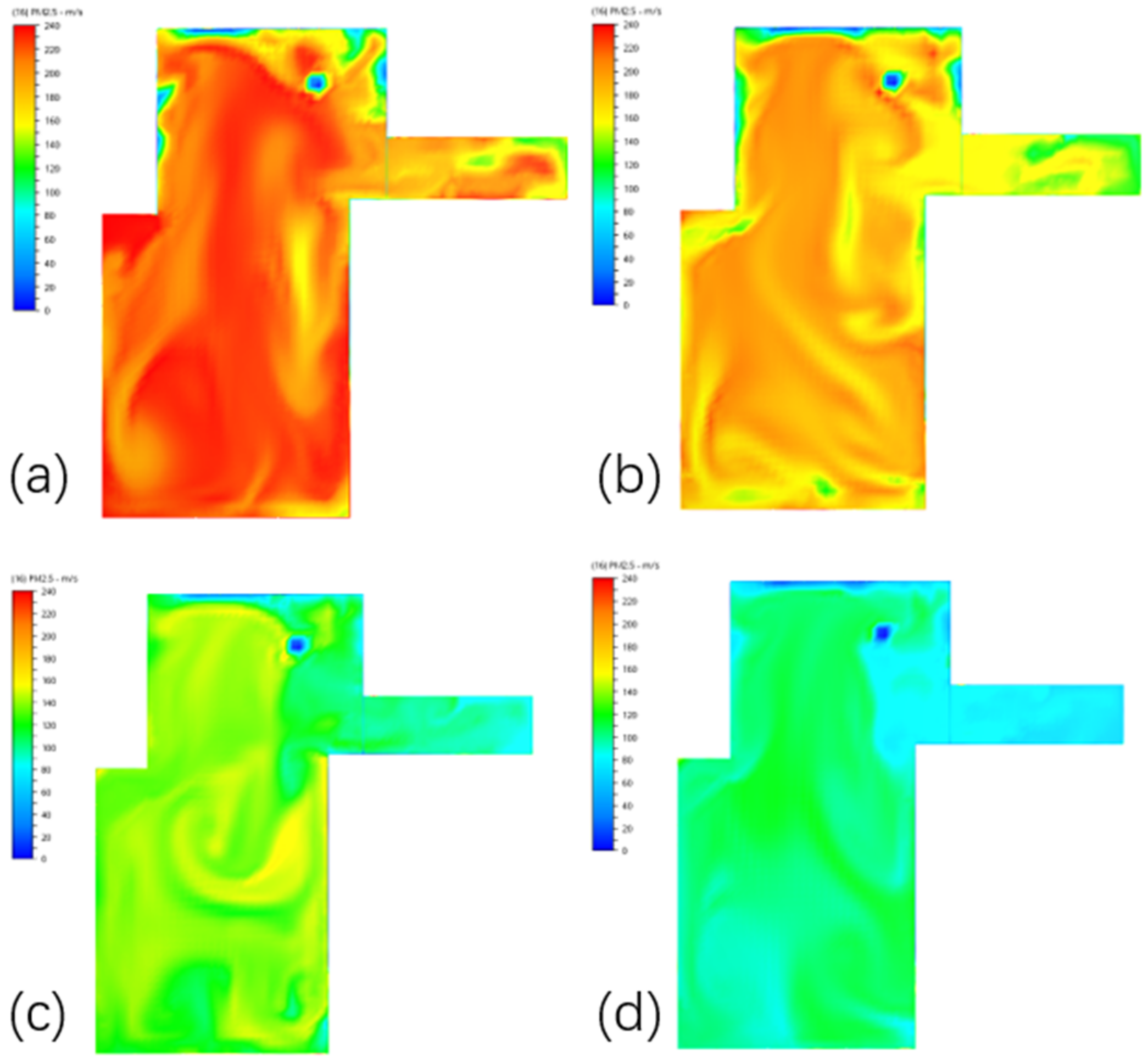
. Figure 9 shows the simulation results at four time stamps (300 s, 600 s, 1200 s, 1800 s) of case 4. It can be seen that the area near the air purification has relatively lower PM2.5 concentration and the distribution of the PM2.5 concentration gradually becomes uniform as time goes on, and the PM2.5 distribution across the whole room evenly becomes uniform.

In contrast, the air purifier in case 9 is located in a side hall of the room, which helps with the air purification of the small region while limiting its efficiency for the whole room. The result can be also seen from the detailed concentration data in each sampling point in Figure A8 in the Appendix A. For example, it can be seen that the average PM2.5 concentration values at points 12 and 13 are 85.3 $\mathsf{\mu }\mathrm{g}/{\mathrm{m}}^3$ and 58.1 $\mathsf{\mu }\mathrm{g}/{\mathrm{m}}^3$ at 30 min, which are significantly lower than other points. The possible reason for case 9 is that the air purifier induced the turbulent airflow in the surrounding area, while the side hall was isolated from the main region of the room, thus the airflow in the side hall could not induce air turbulent flow of a larger region, which reduced the flow rate of PM2.5 into the air purifier.

The rest of the cases (case 1, case 2, case 3, case 5, case 6, case 7, and case 8) achieved similar air purification effects, with the maximum difference within 10 $\mathsf{\mu }\mathrm{g}/{\mathrm{m}}^3$. In addition, the PM2.5 distribution pattern in these cases is also similar: relatively lower in the main region while higher and more uniform in the region of the side hall. The reason is that the air purifier locations in these cases all have efficient effects on the main area of the room and thereby generated higher turbulent flow in the region. Meanwhile, they have limited capability for affecting the space inside the hall, thus high-speed air turbulence was generated there.

The results indicate that for a room with special shapes such as a side hall, the selection of the position for installing an air purifier is very important. The best location would be one that is relatively at the geometric center of the whole area while it needs to be close enough to the side regions. In addition, if the air purifier is located in a small region, it could significantly improve its local efficiency while reducing the overall efficiency across the whole room. Except for specific positions with best or worst air purification effects, the positions of the air purifier in other locations may generate similar effects. However, the above findings are only applicable to the tested air purifier with a centrosymmetric inlet and outlet. If the tested air purifier has a different inlet and outlet, the results may be different.

5. Conclusions

This study proposes a framework to optimize the location of air purifiers for control of indoor PM2.5 based on CFD. Based on the models generated from BIM, the target geometric and semantic information of the rooms are generated, which was integrated into CFD to serve as the simulation environment. Specifications of the air purifier were obtained based on a real typical product. In order to pick the appropriate simulation mode, the simulation results obtained by commonly used simulation models were compared with site measurements. Then the best location, which refers to the purifier placement with the best purification performance, could be found by conducting iterative simulations for each potential location with the selected turbulence model. The framework serves as a generic approach and the slight modifications (e.g., number of mesh grids) could be made for better accuracies to fit similar studies. In addition, a case study was conducted as an illustrative example of the proposed optimization framework. In the case study, the target apartment was empty with no people or furniture. The proposed method can simulate occupied rooms as long as the occupation can be accurately modeled. Some important findings are shown below. Although the findings and quantitative results are only applicable to the simulated apartment of this paper, the proposed optimization approach can be applied to other types of room as well.

• A generally good way to induce an efficient air purification of the room is to place the air purifier at a centered place, while it may have a limited effect on the side halls.
• The efficiency of the air purifier could be very high if it is located in an isolated side hall, though it could not induce an efficient airflow across the whole room, thus eliminating the overall efficiency of the air purification
• In this case study, the best location of the air purifier can increase efficiency by up to 33% compared with other locations.

However, there are some limitations of this study. For example, in the real case, the air purifier may have different options of air inlet or outlet directions, while in this study assumptions regarding the boundary conditions of the air purifier were made. In addition, this study has not considered the effect of natural ventilation in the case that the windows are opened. Therefore, in future studies, the authors plan to incorporate different combinations of natural ventilation and air purifiers as well as different boundary conditions of the air purifiers. In future simulations, the authors will also consider situations when the rooms are occupied by furniture and people.

References

1. Du, Y.; Wan, Q.; Liu, H.; Liu, H.; Kapsar, K.; Peng, J. How does urbanization influence PM2.5 concentrations? Perspective of spillover effect of multi-dimensional urbanization impact. J. Clean. Prod. 2019, 220, 974–983. [Google Scholar] [CrossRef]
2. Oh, H.-J.; Nam, I.-S.; Yun, H.; Kim, J.; Yang, J.; Sohn, J.-R. Characterization of indoor air quality and efficiency of air purifier in childcare centers, Korea. Build. Environ. 2014, 82, 203–214. [Google Scholar] [CrossRef]
3. Franklin, M.; Zeka, A.; Schwartz, J. Association between PM 2.5 and all-cause and specific-cause mortality in 27 US communities. J. Expo. Sci. Environ. Epidemiol. 2007, 17, 279. [Google Scholar] [CrossRef] [PubMed] [Green Version]
4. I, C.A.P.I.I.; Burnett, R.T.; Thun, M.J.; Calle, E.E.; Krewski, D.; Ito, K.; Thurston, G.D. Lung cancer, cardiopulmonary mortality, and long-term exposure to fine particulate air pollution. JAMA 2002, 287, 1132–1141. [Google Scholar]
5. Schwartz, J.; Neas, L.M. Fine Particles Are More Strongly Associated than Coarse Particles with Acute Respiratory Health Effects in Schoolchildren. Epidemiology 2000, 11, 6–10. [Google Scholar] [CrossRef]
6. Adgate, J.L.; Mongin, S.J.; Pratt, G.C.; Zhang, J.; Field, M.P.; Ramachandran, G.; Sexton, K. Relationships between personal, indoor, and outdoor exposures to trace elements in PM2.5. Sci. Total Environ. 2007, 386, 21–32. [Google Scholar] [CrossRef]
7. Zhang, X.; Zhang, X.; Chen, X. Valuing air quality using happiness data: The case of China. Ecol. Econ. 2017, 137, 29–36. [Google Scholar] [CrossRef]
8. Hargreaves, M.; Parappukkaran, S.; Morawska, L.; Hitchins, J.; He, C.; Gilbert, D. A pilot investigation into associations between indoor airborne fungal and non-biological particle concentrations in residential houses in Brisbane, Australia. Sci. Total. Environ. 2003, 312, 89–101. [Google Scholar] [CrossRef] [Green Version]
9. Spalt, E.W.; Curl, C.L.; Allen, R.W.; Cohen, M.; Adar, S.D.; Stukovsky, K.H.; Avol, E.L.; Castro-Diehl, C.; Nunn, C.; Mancera-Cuevas, K.; et al. Time–location patterns of a diverse population of older adults: The Multi-Ethnic Study of Atherosclerosis and Air Pollution (MESA Air). J. Expo. Sci. Environ. Epidemiol. 2015, 26, 349–355. [Google Scholar] [CrossRef] [Green Version]
10. Jones, N.; Thornton, C.; Mark, D.; Harrison, R. Indoor/outdoor relationships of particulate matter in domestic homes with roadside, urban and rural locations. Atmospheric Environ. 2000, 34, 2603–2612. [Google Scholar] [CrossRef]
11. Long, C.M.; Suh, H.H.; Catalano, P.J.; Koutrakis, P. Using Time- and Size-Resolved Particulate Data To Quantify Indoor Penetration and Deposition Behavior. Environ. Sci. Technol. 2001, 35, 2089–2099. [Google Scholar] [CrossRef]
12. Pekey, B.; Bozkurt, Z.; Pekey, H.; Doğan, G.; Zararsız, A.; Efe, N.; Tuncel, G. Indoor/outdoor concentrations and elemental composition of PM10/PM2.5 in urban/industrial areas of Kocaeli City, Turkey. Indoor Air 2010, 20, 112–125. [Google Scholar] [CrossRef]
13. Massey, D.; Masih, J.; Kulshrestha, A.; Habil, M.; Taneja, A. Indoor/outdoor relationship of fine particles less than 2.5μm (PM2.5) in residential homes locations in central Indian region. Build. Environ. 2009, 44, 2037–2045. [Google Scholar] [CrossRef]
14. Zorman, T.; Jeršek, B. Assessment of Bioaerosol Concentrations in Different Indoor Environments. Indoor Built Environ. 2008, 17, 155–163. [Google Scholar] [CrossRef]
15. Martins, N.R.; da Graca, G.C. Impact of PM2.5 in indoor urban environments: A review. Sustain. Cities Soc. 2018, 42, 259–275. [Google Scholar] [CrossRef]
16. Oeder, S.; Dietrich, S.; Weichenmeier, I.; Schober, W.; Pusch, G.; Jörres, R.A.; Schierl, R.; Nowak, D.; Fromme, H.; Behrendt, H.; et al. Toxicity and elemental composition of particulate matter from outdoor and indoor air of elementary schools in Munich, Germany. Indoor Air 2011, 22, 148–158. [Google Scholar] [CrossRef]
17. Abbey, D.E.; Hwang, B.L.; Burchette, R.J.; Vancuren, T.; Mills, P.K. Estimated Long-Term Ambient Concentrations of PM10 and Development of Respiratory Symptoms in a Nonsmoking Population. Arch. Environ. Health Int. J. 1995, 50, 139–152. [Google Scholar] [CrossRef]
18. Matthaios, V.N.; Liu, M.; Li, L.; Kang, C.-M.; Vieira, C.L.; Gold, D.R.; Koutrakis, P. Sources of indoor PM2.5 gross α and β activities measured in 340 homes. Environ. Res. 2021, 197, 111114. [Google Scholar] [CrossRef]
19. Colome, S.D.; Kado, N.Y.; Jaques, P.; Kleinman, M. Indoor-outdoor air pollution relations: Particulate matter less than 10 μm in aerodynamic diameter (PM10) in homes of asthmatics. Atmospheric Environ. Part A. Gen. Top. 1992, 26, 2173–2178. [Google Scholar] [CrossRef]
20. Jones, A.P. Indoor air quality and health. Atmos. Environ. 1999, 33, 4535–4564. [Google Scholar] [CrossRef]
21. A Wallace, L.; Emmerich, S.J.; Howard-Reed, C. Continuous measurements of air change rates in an occupied house for 1 year: The effect of temperature, wind, fans, and windows. J. Expo. Sci. Environ. Epidemiol. 2002, 12, 296–306. [Google Scholar] [CrossRef] [PubMed]
22. Weerasuriya, A.; Zhang, X.; Gan, V.J.; Tan, Y. A holistic framework to utilize natural ventilation to optimize energy performance of residential high-rise buildings. Build. Environ. 2019, 153, 218–232. [Google Scholar] [CrossRef]
23. Park, J.S.; Jee, N.-Y.; Jeong, J.-W. Effects of types of ventilation system on indoor particle concentrations in residential buildings. Indoor Air 2014, 24, 629–638. [Google Scholar] [CrossRef] [PubMed]
24. Ye, W.; Zhang, X.; Gao, J.; Cao, G.; Zhou, X.; Su, X. Indoor air pollutants, ventilation rate determinants and potential control strategies in Chinese dwellings: A literature review. Sci. Total. Environ. 2017, 586, 696–729. [Google Scholar] [CrossRef] [PubMed]
25. Zhao, Y.; Sun, H.; Tu, D. Effect of mechanical ventilation and natural ventilation on indoor climates in Urumqi residential buildings. Build. Environ. 2018, 144, 108–118. [Google Scholar] [CrossRef]
26. Cooper, E.; Milner, J.; Wang, Y.; Stamp, S.; Mumovic, D. Modelling the impact on mortality of using portable air purifiers to reduce PM2.5 in UK homes. Atmospheric Environ. 2022, 289, 119311. [Google Scholar] [CrossRef]
27. Quang, T.N.; He, C.; Morawska, L.; Knibbs, L.D. Influence of ventilation and filtration on indoor particle concentrations in urban office buildings. Atmos. Environ. 2013, 79, 41–52. [Google Scholar] [CrossRef] [Green Version]
28. Stephens, B.; Siegel, J.A. Penetration of ambient submicron particles into single-family residences and associations with building characteristics. Indoor Air 2012, 22, 501–513. [Google Scholar] [CrossRef]
29. Rice, J.L.; Brigham, E.; Dineen, R.; Muqueeth, S.; O’Keefe, G.; Regenold, S.; Koehler, K.; Rule, A.; McCormack, M.; Hansel, N.N.; et al. The feasibility of an air purifier and secondhand smoke education intervention in homes of inner city pregnant women and infants living with a smoker. Environ. Res. 2017, 160, 524–530. [Google Scholar] [CrossRef] [Green Version]
30. Shaughnessy, R.; Sextro, R. What is an effective portable air cleaning device? A review. J. Occup. Environ. Hyg. 2006, 3, 169–181. [Google Scholar] [CrossRef]
31. Mamaghani, A.H.; Haghighat, F.; Lee, C.-S. Photocatalytic degradation of VOCs on various commercial titanium dioxides: Impact of operating parameters on removal efficiency and by-products generation. Build. Environ. 2018, 138, 275–282. [Google Scholar] [CrossRef]
32. Zhou, B.; Liu, T.; Yi, S.; Huang, Y.; Guo, Y.; Huang, S.; Zhou, C.; Zhou, R.; Cao, H. Reducing the effectiveness of ward particulate matter, bacteria and influenza virus by combining two complementary air purifiers. Int. J. Environ. Res. Public Health 2022, 19, 10446. [Google Scholar] [CrossRef]
33. Lee, Y.-W.; Kim, Y.-S.; Han, B.; Kim, Y.-J.; Kim, H.-J. Minimizing the Size and Ozone Emission of Electrostatic Precipitators Using Dielectric and Rolled Carbon Film Coatings. IEEE Trans. Ind. Appl. 2021, 58, 753–759. [Google Scholar] [CrossRef]
34. Baranowska-Wójcik, E.; Szwajgier, D.; Oleszczuk, P.; Winiarska-Mieczan, A. Effects of Titanium Dioxide Nanoparticles Exposure on Human Health—A Review. Biol. Trace Elem. Res. 2020, 193, 118–129. [Google Scholar] [CrossRef] [Green Version]
35. Yan, S.; Liu, C.; Hou, L.-A.; Wang, B.; Zhang, Y. A new filterless indoor air purifier for particulate matter and bioaerosol based on heterogeneous condensation. Environ. Res. 2023, 218, 115034. [Google Scholar] [CrossRef]
36. Wadchasit, P.; Khamwichit, W.; Sanongraj, W. The Synthesis of Air Filters from Silk Cocoons Coated TiO2 for Use in Air Purifier. Adv. Mater. Res. 2014, 931–932, 281–285. [Google Scholar] [CrossRef]
37. Novoselac, A.; Siegel, J.A. Impact of placement of portable air cleaning devices in multizone residential environments. Build. Environ. 2009, 44, 2348–2356. [Google Scholar] [CrossRef]
38. Wilcox, D.C. Turbulence Modeling for CFD; DCW industries: La Canada, CA, USA, 1998. [Google Scholar]
39. Yakhot, V.; Orszag, S.; Thangam, S.; Gatski, T.; Speziale, C. Development of turbulence models for shear flows by a double expansion technique. Phys. Fluids A Fluid Dyn. 1992, 4, 1510–1520. [Google Scholar] [CrossRef] [Green Version]
40. Menter, F.R. Two-equation eddy-viscosity turbulence models for engineering applications. AIAA J. 1994, 32, 1598–1605. [Google Scholar] [CrossRef]
41. Bertin, J.J.; Periaux, J.; Ballmann, J. Advances in Hypersonics: Modeling Hypersonic Flows; Springer: Berlin/Heidelberg, Germany, 1992. [Google Scholar]
Figure 1. The proposed framework for operation optimization of air purifiers.
Buildings 13 00077 g001
Figure 2. (a) 3D view of the selected room; (b) floor plan of the selected room (unit is m).
Buildings 13 00077 g002
Figure 3. BIM model of the selected air purifier and corresponding properties.
Buildings 13 00077 g003
Figure 4. (a) Tested locations of the air purifier; (b) observation points in the apartment.
Buildings 13 00077 g004
Figure 5. (a) 3D model of the tested apartment; (b) mesh of the computational domain.
Buildings 13 00077 g005
Figure 6. Quantitative results of the nine cases at 1800 s.
Buildings 13 00077 g006
Figure 7. The average concentration of PM2.5 at different times.
Buildings 13 00077 g007
Figure 8. The convergence curve for case 4 simulation.
Buildings 13 00077 g008
Figure 9. The simulation results of case 4 at the time of (a) 300 s; (b) 600 s; (c) 1200 s; (d) 1800 s.
Buildings 13 00077 g009