An Evolutionary Neuro-Fuzzy-Based Approach to Estimate the Compressive Strength of Eco-Friendly Concrete Containing Recycled Construction Wastes

Abstract

There has been a significant increase in construction and demolition (C&D) waste due to the growth of cities and the need for new construction, raising concerns about the impact on the environment of these wastes. By utilising recycled C&D waste, especially in concretes used in construction, further environmental damage can be prevented. By using these concretes, energy consumption and environmental impacts of concrete production can be reduced. The behaviour of these types of concrete in laboratories has been extensively studied, but reliable methods for estimating their behaviour based on the available data are required. Consequently, this research proposes a hybrid intelligent system, Fuzzy Group Method of Data Handling (GMDH)–Horse herd Optimisation Algorithm (HOA), for predicting one of the most important parameters in concrete structure design, compressive strength. In order to avoid uncertainty in the modelling process, crisp input values were converted to Fuzzy values (Fuzzification). Next, using Fuzzy input variables, the group method of data handling is used to predict the compressive strength of recycled aggregate concrete. The HOA algorithm is one of the newest metaheuristic algorithms being used to optimise the Fuzzy GMDH structure. Several databases containing experimental mix design records containing mixture components are gathered from published documents for compressive strength to assess the accuracy and reliability of the proposed hybrid Fuzzy-based model. Compared to other original approaches, the proposed Fuzzy GMDH model with the HOA optimiser outperformed them in terms of accuracy. A Monte Carlo simulation is also employed for uncertainty analysis of the empirical, standalone, and hybridised models in order to demonstrate that the evolutionary Fuzzy-based approach has less uncertainty than the standalone methods when simulating compressive strength.

1. Introduction

Global climate change is affecting many countries [1,2]. Thus, global collaboration has been initiated to support low-carbon sustainable development in response to this grand challenge [3]. The construction sector, however, cannot be excluded from these mitigation strategies as this industry is responsible for a high portion of global carbon emissions [4,5]. Cement is a significant source of carbon dioxide emitted during production and consumption [6]. Thus, employing some strategies such as using recycled materials could substantially reduce greenhouse gas emissions in this sector [7,8]. There are many studies that address how the construction sector can reduce global warming’s impacts, but there are few studies that address the use of recycled materials in this area [9]. Alternative materials, recycled waste concrete, can be substituted for conventional concrete constituents to alleviate the aforementioned issues and improve sustainability.

Different studies were carried out to discuss and evaluate the technological feasibility of Recycled Construction and Demolition Waste Aggregate Concrete (RCDWAC) [10,11,12,13,14]. The mechanical characteristics of RCDWAC may be generally less than those of Ordinary Portland Concrete (OPC), but they are still adequate for some practical construction alternatives [15]. 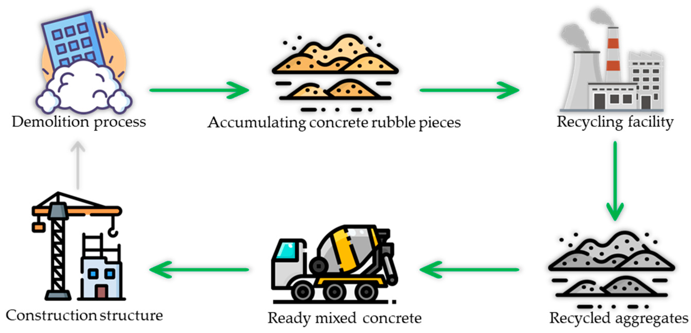A recycling station and concrete factory are used to produce RCDWAC, which incorporates natural coarse aggregates [16]. Two stages were involved in the demolition waste concrete recycling process. Crushing with jaw crushers (first) and crushing with impact crushers (second). Engineering tools (e.g., electromagnets, water cleaners, or air sifters) were used to remove reinforcement and contaminants after crushing [17]. Figure 1 illustrates the reproducing cycle of RCDWAC. Although studies on these concrete types have already begun, their characteristics remain unclear. Characteristics of concrete are input parameters in a number of design codes [18]. It is, therefore, crucial that these characteristics are accurately estimated so as to save time and effort [19]. Predicting concrete characteristics has been the focus of the majority of earlier studies [20]. Models previously published for regular concrete may, however, fail to accurately estimate the characteristics of other types of concrete.

The mechanical behaviour of concrete is dependent on experimental characteristics such as volumetric/weighted mixture proportion values [21]. Developing cost-effective and eco-friendly cementitious blends with optimal structural performance is a crucial objective for researchers and engineers [22]. Complex standards necessitate specialised users and time-consuming procedures for experimental investigation. Therefore, civil engineers employed an eco-friendly solution based on the development of Artificial Intelligence (AI) models to address this issue [23,24,25,26,27,28,29,30]. Several linear and nonlinear regression-based AI methods have recently been utilised to model concrete’s mechanical and structural properties. Sadowski et al. [31] estimated the compressive strength (CS) of low-strength concrete containing mineral dusts using the hybridised model. DeRousseau et al. [32] tried to compare predictive regression-based artificial intelligence models to simulate the compressive strength of field-placed concrete. Shahmansouri et al. [33] proposed Artificial Neural Network (ANN) and Gene Expression Programming (GEP) techniques for eco-environmentally concrete properties. The authors of [34] introduced a novel method for predicting the compressive strength (CS) of foam lightweight concrete based on an optimisation algorithm and Multivariate Adaptive Regression Splines (MARS). Naseri et al. [35] employed machine learning and evolutionary approaches for designing sustainable mixtures. Dao et al. [36] investigated Adaptive Neuro-Fuzzy Inference System (ANFIS) and ANN to estimate the behaviour of geopolymer concrete. Asteris and Mokos [37] employed an ANN system as an alternative application for estimating the CS of concrete using a non-destructive experimental method. Golafshani et al. [38] estimated the compressive strength (CS) of ordinary and high-performance concretes employing evolutionary methods. Behnood and Golafshani [39] studied the M5p model tree method to simulate the mechanical properties of mixtures containing waste foundry sand. Asteris and Mokos [37] presented a surrogate model for the estimation of the compressive strength of masonry. Feng et al. [40] evaluated an adaptive boosting technique for estimating the compressive strength of concrete containing granulated blast furnace slag. Li et al. [41] examined the ability of data-driven models known as ANN, ANFIS, and Multiple Linear Regression (MLR) to predict the service life of concrete. Using the GEP concept, Gholampour et al. [42] formulated the compressive strength of recycled aggregate concrete with non-pozzolanic admixtures. Al-Shamiri et al. [43] presented the Extreme Learning Method (ELM) and ANN for predicting the CS of cylindrical samples of high-strength concrete.

Although the AI models mentioned above have been successfully applied to a wide variety of civil engineering problems, many rely on crisp input variables to model the target variables, which can be a limitation of the modelling [44]. In contrast to their crisp counterparts, Fuzzy sets have gradual transitions between defined sets; this enables the uncertainty associated with these concepts to be directly modelled. After defining each model variable with a series of overlapping Fuzzy sets, the mapping of inputs to outputs can be expressed as a set of IF-THEN rules, which can be specified entirely from expert knowledge or from data [45]. However, unlike NNs, Fuzzy models are prone to a rule explosion; that is, as the number of variables or Fuzzy sets per variable increases, there is an exponential increase in the number of rules [46].

The main aim of this study is to develop a sustainable and predictive method for assessing the CS of RCDWAC using a hybridised and self-tuned model. To the authors’ knowledge, a hybridised Fuzzy GMDH coupled with HOA has not previously been developed and applied in modelling sustainable technology. During the calibration stage, the trial-and-error procedure for the hyperparameter setting for each model prevented ANFIS and GMDH models from performing satisfactorily for CS prediction. To overcome this shortcoming, HOA, a new metaheuristic method, is applied to explore for appropriate values of the user-defined parameters of the proposed model. HOA is a low-cost algorithm with a high degree of convergence that was first introduced in 2021 [47]. Then, the hybrid Fuzzy GMDH-HOA results are compared to those extracted from ELM, ANFIS, GMDH, and empirical equations by [42,48,49]. In this research, sensitivity analysis and parametric study were conducted to investigate and determine the most effective input variables (RCDWAC mix properties) and the influence of RCDWA on CS.

The remaining sections of the paper are as follows: Section 2 proposes a theoretical framework, existing models, an RCDWAC dataset, and a statistical description of used data; Section 3 describes the AI development and evaluation of proposed approaches for CS of RCDWAC; and Section 4 concludes with a conclusion, research highlights, and limitations.

2. Materials and Methods

2.1. Theoretical Framework and Existing Models

Until 2015, the global consumption of aggregates for construction and maintenance of civil engineering projects is anticipated to increase by over 5.2% per year, reaching 48.3 billion tonnes [50,51]. According to Eurostat (https://ec.europa.eu/eurostat, accessed on 23 June 2022), Europe produced approximately 2.5 billion tonnes of waste in 2010, of which about 860 million tonnes were demolition waste from the construction industry. According to this challenge, one of the most impressive, cost-effective, and environmentally friendly activities for the sustainable development of the concrete industry [48] is using recycled aggregate in concrete production. Based on this sustainable concept, experimental and artificial intelligence investigations were conducted to evaluate the strength behaviour of RCDWAC using formula-based models. In structural challenges, estimating CS at various ages is a significant concern. The following formula was proposed by ACI Committee 209 [48] for calculating the compressive strength of Portland cement-based concrete. In this formula, (t) refers to the age of specimens and ($C{S}_{28}$) is the 28-day compressive strength.

$$CS \left(t\right)=\frac{AS}{4+0.85\times AS}\times C{S}_{28}$$

(1)

Gholampour, Gandomi, and Ozbakkaloglu [42] presented a predictive equation for RCDWAC based on experimental variables such as the water-to-cement ratio and recycled aggregate using the AI method.

$$CS=\frac{19.1\times {0.998}^{\%RA}\times (\frac{W}{C}+0.33)}{{\frac{W}{C}}^{1.5}}$$

(2)

Abdollahzadeh, Jahani, and Kashir [49] investigated experimental factors (246.2 > W (Kg/m³) > 113, 500 > C (Kg/m³) > 250, 1797.7 > RA (Kg/m³) > 0 and 90 > AS (day) > 3) to propose a linear relationship for CS of RCDWAC.

$$CS=\sqrt{RA-\left(W-\left(CA+FA\right)\right)+(AS\times 18.908})+\left(\left(-9.989\right)-\frac{9.989}{AS}\right)$$

(3)

2.2. Description of Dataset

Using experimental data records from RCDWAC mixtures to simulate the hardened behaviour of concrete, this study implemented AI techniques based on the regression concept. Therefore, instances of data were extracted from the document that had been peer-reviewed [52,53,54,55,56,57,58,59,60,61,62,63,64,65,66,67]. Based on gathered data records, the predictive standalone and evolutionary approaches of CS for RCDWAC were applied to 353 experimental records of varying ages, utilising 353 experimental records. The dataset included influencing parameters regarding mixture constituents of RCDWAC in numerous constituents. The collected dataset is split into two subsets. The calibration subset is created for system knowledge implementation and developing a CS regression model. The validation subset is implemented to assess the performance capability of the proposed RCDWAC property models. The calibrating subset consisted of approximately 75% of the CS data instances (266 records). Alternatively, regression-based AI methods were validated using the remaining 87 records. Using

Table 1. Statistical measures of inputs and outputs in this study.

Variables	W (kg/m3)	C (kg/m3)	FA (kg/m3)	CA (kg/m3)	RA (kg/m3)	AS (days)	CS (MPa)
Minimum	120	220	365	0	0	7	13
Median	180	400	720	629.5	443.7	28	41.2
Maximum	244	750	1020	1366	1259	180	88.3
Range	124	530	655	1366	1259	173	75.3
Mean	184.1	394.9	710.3	564.8	504.3	45.25	42.11
Std. Deviation	27.14	83.94	108.5	438.7	414.6	43.96	13.13
Std. Error of Mean	1.444	4.468	5.772	23.35	22.07	2.34	0.6986
Skewness	0.288	1.111	0.3158	−0.1004	0.2203	1.783	0.6451
Kurtosis	0.3913	2.982	1.499	−1.453	−1.412	2.252	0.778

and Equation (4), the effective components for optimal concrete design are reported. The statistical measures of the most effective variables to design concrete with optimal mechanical properties such as cement (C), water (W), coarse aggregate (CA), fine aggregate (FA), recycled aggregate (RA), and age of specimens (AS), are presented in Table 1.

Moreover, the heatmap in Figure 2 illustrates the Pearson correlation analysis of selected inputs used to develop the models. The correlation heatmap demonstrates no significant correlations between the selected matrices and CS.

$$CS=f\left(W,C,FA,CA,RA,AS\right)$$

(4)

In addition, the Pearson correlation analysis of selected inputs for developing regression-based AI models is displayed on a heatmap in Figure 2. As stated by the correlation heatmap, there are no significant correlations between the selected matrices and CS, so it is best to consider all six parameters when modelling CS. Moreover, the histogram of CS values presented in Figure 2 revealed that the greatest frequency of CS dispersion occurred between 32.5 and 45.5 Mpa.

3. Methodology

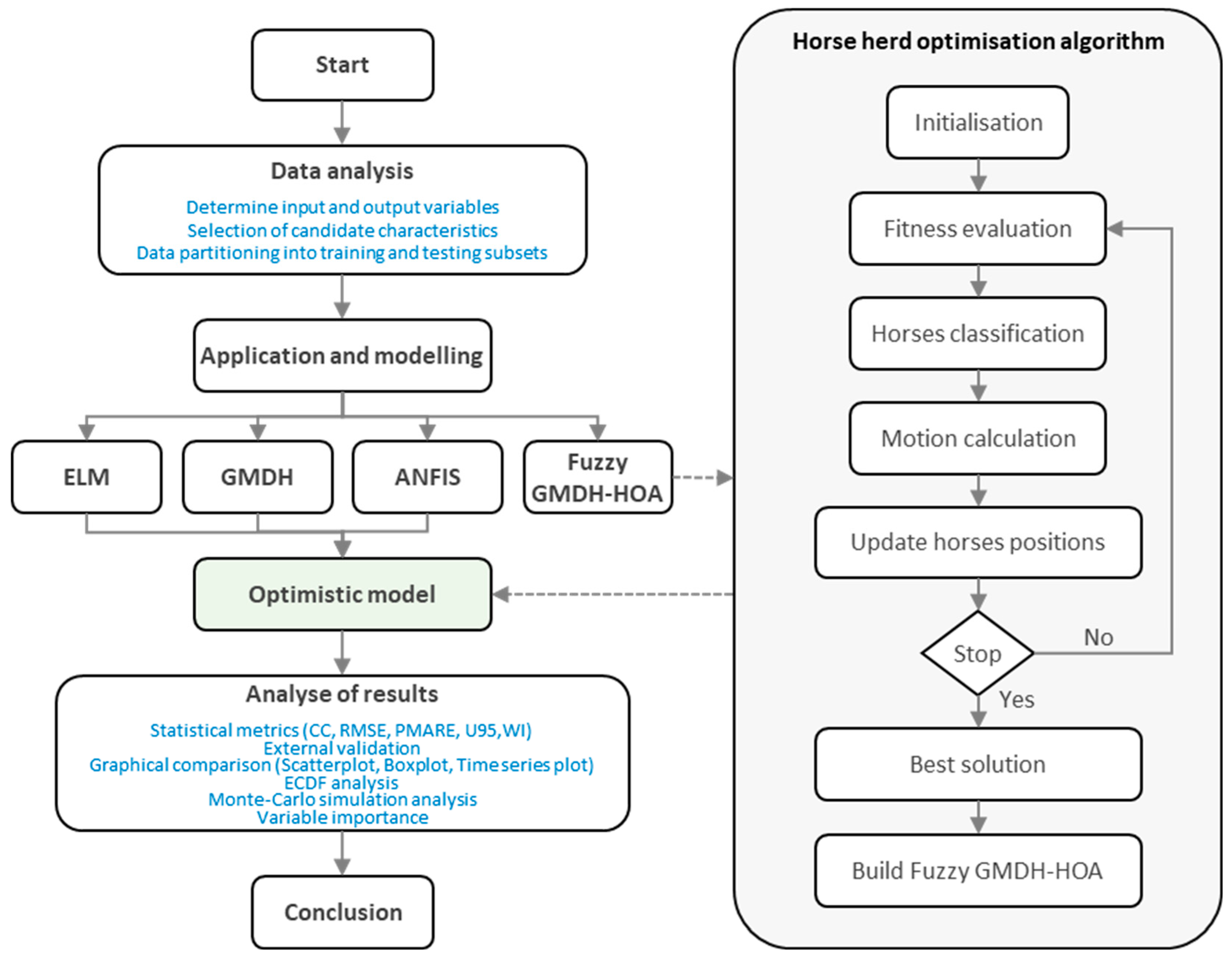
Several AI models, including GMDH, ANFIS, ELM, and hybridised Fuzzy GMDH-HOA, are used in the current study to model the CS of concrete made with recycled wastes from the demolition of structures. In this subsection, the context of the discussed models is presented. In addition, Figure 3 explains the workflow corresponding to the introduced models in this study.

3.1. Extreme Learning Machine (ELM)

Huang et al. [68] developed the ELM algorithm for determining the weight of a hidden neuron. It substantially reduces the required calculation time for training and selecting the model structure for large numbers. In addition, its implementation is relatively straightforward [69,70,71]. With a network containing c outputs, hidden neurons and p input units, the i-th output at time step zero is calculated as follows:

$$o_i\left(t\right)=m_i^{T}h\left(t\right)$$

(5)

In the above equation $m_i ϵ {ℝ}^q, \forall i ϵ \left\{1, \dots , c\right\}$ denotes the weight vector and relates the hidden neurons to the $i^{th}$ output neuron. $h\left(t\right)ϵ {ℝ}^q$ denotes the hidden neuron output of an input pattern $X\left(t\right)ϵ {ℝ}^q$ in the data set ${\left\{X\left(t\right)\right\}}_{t=1}^n$. Vector h(t) is expressed as:

$$h\left(t\right)={\left[f\left(W_1^{T}X\left(t\right)+b_1\right),f\left(W_2^{T}X\left(t\right)+b_2\right),\dots ,f\left(W_q^{T}X\left(t\right)+b_q\right)\right]}^T$$

(6)

Here, b_l denotes the bias of the l-th hidden neuron, $W_l ϵ {ℝ}^q$ denotes the weight vector of the l-th hidden neuron; finally, $f(.)$ represents a sigmoidal activation distribution. The weight vectors (wl) are now randomly derived from a normal or uniform distribution. In addition, $H=\left[h\left(1\right)h\left(2\right)\dots h\left(n\right)\right]$ is a $q\times n$ matrix. In this matrix, the t-th column represents the hidden-layer vector $h\left(t\right)ϵ{ℝ}^q$. In a similar way, $D=\left[\mathrm{d}\left(1\right)\mathrm{d}\left(2\right)\dots \mathrm{d}\left(\mathrm{n}\right)\right]$ denotes a $c\times n$ matrix in which the t-th column is the target or desired vector $d\left(t\right)ϵ{ℝ}^c$ which is related to the input pattern $x\left(t\right),t=1,\dots ,N$. Ultimately $M=\left[m\left(1\right)m\left(2\right)\dots m\left(c\right)\right]$ is a $q\times c$ matrix. The i-th column of this matrix is the weight vector, $m_iϵ{ℝ}^q,i=1,\dots ,c$. These three matrices are associated with each other through linear mapping.

$$D=M^{T}H$$

(7)

Based on the available data, D and H are known matrices, whereas M is unknown, but can be calculated using the Moore–Penrose pseudo-inverse method.

$$M={\left(H{H}^T\right)}^{-1}H{D}^T$$

(8)

If we assume that the number of output neurons equals the number of classes, we can calculate the class index i* for a new input pattern using the following formula:

$$i^{*}=arg\underset{i=1,\dots ,c}{\max }\left\{O_i\right\}$$

(9)

where Equation (5) is used for the calculation of $o_i$.

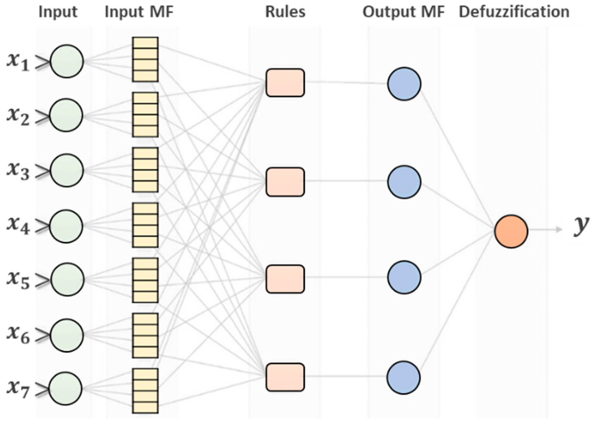
3.2. Adaptive Neuro-Fuzzy Inference System (ANFIS)

ANFIS is a type of ANN that combines neural networks and Fuzzy logic [72]. Jang [73] developed ANFIS in 1993 to model nonlinear functions, forecast chaotic time series, and identify nonlinear components. Using the Takagi–Sugeno inference system (expressed as Fuzzy If-Then rules) [74], ANFIS could be used to construct an input–output mapping. Numerous benefits of ANFIS, including the ability to catch the nonlinear structure of a procedure, accelerated learning, and adaptability, have led to its widespread use among engineers [75]. The core of ANFIS is the FIS (Fuzzy Inference System). In the initial layer, inputs are received and converted to Fuzzy values using MFs (Membership Functions). The rule base consists of two Fuzzy IF-Then rules of the Takagi and Sugeno varieties:

• $Rule1:ifxis{A}_{1}andyis{B}_1,then{f}_1=p_{1}x+q_{1}y+r_1.$
• $Rule2:ifxis{A}_{2}andyis{B}_2,then{f}_2=p_{2}x+q_{2}y+r_2$.

Each node on the first layer is selected as an adaptive node with a function.

$$O_i^1=\mu A_i\left(s\right)$$

(10)

In the preceding expression, $O_i^1$ represents the membership function of the linguistic label A_i. Gaussian functions (also known as bell-shaped functions) are frequently used in ANFIS due to their greater capacity in nonlinear data regression [75]. The following defines a bell-shaped function with a minimum value of zero and a maximum value of one:

$$\mu \left(x\right)=bell\left(x;a_i,b_i,c_i\right)=\frac{1}{1+{[(\frac{x-c_1}{a_i})]}^{b_i}}$$

(11)

In the expression above, x represents the input and {$a_i,b_i,c_i$} represent the set parameters. The incoming signals are multiplied in the second layer, and the resulting product is transmitted to the third layer. The third layer, the rule layer, computes the ratio of the i-th node’s firing strength to that of the other nodes. The fourth layer is the defuzzification layer, where each node has a node function. The fifth output layer is responsible for calculating the total output, which is the sum of all incoming signals. The current procedure selects a threshold value between the actual and output values. The subsequent parameters are then calculated using the least-squares method, which produces an error for each calculated value. If the obtained value exceeds the threshold value, a gradient descent algorithm [76,77] is used to update the assumed parameters. The procedure is repeated until the error value falls below the threshold value. This method’s parameters are simultaneously calculated and controlled utilising the least-square and gradient descent algorithms.

3.3. Group Method of Data Handling (GMDH)

A self-organising algorithm was initially developed by Ivahnenko. Typically, it is based on self-organising systems [78]. The model can generate quadratic polynomials in any neuron called Partial Descriptions (PDs) to select neurons with the best fit values, as well as generate error criteria to terminate the training phase and form a tree-like structure to solve highly complex problems [79,80]. A function of $\widehat{f}$ can be substituted for the actual function f in order to predict the final output of a complex system, $\widehat{y}$, for given model input, $X=\left(x_1, x_2, \dots , x_n\right)$, so that it is as close as possible to its actual output, y. Consequently, for given n observations of multi-variable data, the output variable is represented as follows:

$$y_i=f\left(x_{i1}, x_{i2}, \dots , x_{in}\right), i=1,2,3,\dots ,M$$

(12)

In the current status, the model of GMDH can be well-constructed to predict the final values of output, ${\widehat{y}}_i$, in the case of each given input vector $X=\left(x_{i1}, x_{i2}, \dots , x_{in}\right)$. A relationship between the final output and the inputs can be defined using the following function:

$${\widehat{y}}_i=\widehat{f}\left(x_{i1}, x_{i2}, \dots , x_{in}\right), i=1,2,3,\dots ,M$$

(13)

Based on the measured (observed) values and predicted model outputs, the following equation represents the error values:

$${\displaystyle \sum }_{i=1}^M{\left[\widehat{f}\left(x_{i1}, x_{i2}, \dots , x_{in}\right)-y_i\right]}^2 \to min$$

(14)

According to the GMDH model, dependent and independent parameters are related as follows:

$$y=w_0+{\displaystyle \sum }_{i=1}^n{w}_i{x}_i+{\displaystyle \sum }_{i=1}^n{\displaystyle \sum }_{j=1}^n{w}_{ij}{x}_i{x}_j+{\displaystyle \sum }_{i=1}^n{\displaystyle \sum }_{j=1}^n{\displaystyle \sum }_{k=1}^n{w}_{ijk}{x}_i{x}_j{x}_k+\dots ,$$

(15)

In addition, Equation (5) is suggested as the Kolmogorov–Gabor polynomial [78]. A quadratic polynomial has a lower error rate than other types of polynomials, and its weighting coefficients are calculated by least squares. For each pair of input variables $x_i$ and $x_j$, the error between the actual value and predicted model output y should be minimised. Additionally, this error function can determine the performance of a quadratic polynomial, $G_i$, using the least-square method to optimally remove a specified number of neurons (nodes) from each layer, as shown below:

$$E=\frac{{{\displaystyle \sum }}_{i=1}^M{(y_i-G())}^2}{M} \to min$$

(16)

When building the regression quadratic polynomial in GMDH, all possible independent variables (or inputs) are considered out of n input variables [80]. Weighting coefficients were derived using the least squares method in this case. The number of nodes in each layer can be calculated as follows:

$$C_n^2=n\left(n-1\right)/2,$$

where $n$ stands for the input numbers of the former layer. However, the partial descriptions will be produced in the initial layer from observations $\left\{\left(y_i{x}_{ip}{x}_{iq}\right);\left(1, 2, \dots , M\right)\right\}$ for different pairs of $p, q \in \left\{1, 2, \dots , n\right\}$. In other words, $M$ triples $\left\{\left(y_i{x}_{ip}{x}_{iq}\right);\left(1, 2, \dots , M\right)\right\}$ could be formed as inputs–output systems from n observations using $p, q \in \left\{1, 2, \dots , n\right\}$, expressed as follows [75,76,77]:

$$\left[\begin{array}{ccc}{x}_{1p}& x_{1q}& y_1\\ x_{2p}& x_{2q}& y_2\\ .& .& .\\ x_{mp}& x_{mq}& y_m\end{array}\right]$$

(17)

Considering coefficients of the weighting of the quadratic polynomial $W={\left\{w_0, w_1,\dots , w_5 \right\}}^{Tr}$, a mathematical matrix equation AW = Y, and the vector of output $Y={\left\{y_1, y_2,\dots , y_M \right\}}^{Tr}$, the final matrix created by combining two inputs can be determined as follows:

$$\left[\begin{array}{cccccc}1& x_{1p}& x_{1q}& x_{1p}.x_{1q}& x_{1p}^2& x_{1q}^2\\ 1& x_{2p}& x_{2q}& x_{2p}.x_{2q}& x_{2p}^2& x_{2q}^2\\ .& .& .& .& .& .\\ 1& x_{mp}& x_{mq}& x_{mp}.x_{mq}& x_{mp}^2& x_{mq}^2\end{array}\right]$$

(18)

The coefficients vector of $W={\left(A^{Tr}A\right)}^{-1}{A}^{Tr}Y$ can be calculated using the least-squares approach.

3.4. Horse Herd Optimisation Algorithm (HOA)

Metaheuristic algorithms have been developed and used for a wide range of complex engineering problems in recent years [81,82,83,84,85,86]. Developed by [47], HOA is based on the horses’ observed behaviour patterns in their environment. The six most important behavioural patterns of horses are hierarchy, sociability, grazing, imitation, defence mechanism, and roaming, and the HOA is based on these behaviours. The movement applied to the horses during each iteration (Equation (19)) is as follows:

$$X_m^{Iter,AGE}={\overrightarrow{V}}_m^{Iter,AGE}+X_m^{\left(Iter-1\right),AGE} , AGE=\alpha ,\beta ,\gamma ,\delta$$

(19)

In the above equation, $X_m^{Iter, AGE}$ denotes the m-th horse position, Iter denotes the current iteration, and AGE represents the range of age for the considered horse and ${\overrightarrow{V}}_m^{Iter,AGE}$ represents the velocity vector of the considered horse. Each horse has a maximum life of 25–30 years, so it could exhibit various behaviours during its lifetime [47]. Thus, $\delta$ represents a life range of 0–5 years, $\gamma$ represents a life range of 5–10 years, and $\alpha$ represents horses that are older than 15 years. A comprehensive and large response matrix is executed per iteration to determine the horses’ ages. In this respect, the matrix is sorted in terms of best responses. From the sorted matrix, the first 10% of horses are selected, representing the $\alpha$ horses. Consequently, the following 20% fall in the $\beta$ group. Additionally, the remaining 30% and 40% of horses belong to $\gamma$ and $\delta$ horses, respectively. The motion vectors of horses per different ages and at each cycle of the algorithm could be written as follows based on the above-mentioned horse behaviours (Equation (19))

$$\begin{array}{l}{\overrightarrow{V}}_m^{Iter,\alpha }={\overrightarrow{G}}_m^{Iter,\alpha }+{\overrightarrow{D}}_m^{Iter,\alpha }\\ {\overrightarrow{V}}_m^{Iter,\beta }={\overrightarrow{G}}_m^{Iter,\beta }+{\overrightarrow{H}}_m^{Iter,\beta }+{\overrightarrow{S}}_m^{Iter,\beta }+{\overrightarrow{D}}_m^{Iter,\beta }\\ {\overrightarrow{V}}_m^{Iter,\gamma }={\overrightarrow{G}}_m^{Iter,\gamma }+{\overrightarrow{H}}_m^{Iter,\gamma }+{\overrightarrow{S}}_m^{Iter,\gamma }+{\overrightarrow{I}}_m^{Iter,\gamma }+{\overrightarrow{D}}_m^{Iter,\gamma }+{\overrightarrow{R}}_m^{Iter,\gamma }\\ {\overrightarrow{V}}_m^{Iter,\delta }={\overrightarrow{G}}_m^{Iter,\delta }+{\overrightarrow{I}}_m^{Iter,\delta }+{\overrightarrow{R}}_m^{Iter,\delta }\end{array}$$

(20)

Using Equations (21) and (22) to explain how the global matrix is derived, positions (X) are juxtaposed with the cost of each position (C(X)).

$$X=[\begin{array}{cccc}{x}_{1,1}& x_{1,2}& \cdots & x_{1,d}\\ x_{2,1}& x_{2,2}& \cdots & x_{2,d}\\ ⋮& ⋮& \ddots & ⋮\\ x_{m,1}& x_{m,2}& \cdots & x_{m,d}\end{array}],C\left(X\right)=\left[\begin{array}{c}{c}_1\\ c_2\\ ⋮\\ c_m\end{array}\right]$$

(21)

$$GlobalMatrix=\left[\begin{array}{cc}X& C\end{array}\left(X\right)\right]=\left[\begin{array}{ccccc}{x}_{1,1}& x_{1,2}& \cdots & x_{1,d}& c_1\\ x_{2,1}& x_{2,2}& \cdots & x_{2,d}& c_2\\ ⋮& ⋮& \ddots & ⋮& ⋮\\ x_{m,1}& x_{m,2}& \cdots & x_{m,d}& c_{\mathrm{m}}\end{array}\right]$$

(22)

As shown in the preceding equations, x represents the position and c(x) represents the cost of each position. Moreover, m and d represent the number of horses and the dimensions of the problem. Next, we would store the global matrix according to the last column, which represents costs. The age of the horse is entered here.

In situations where an optimal solution has a high probability, high accuracy and low speed are advantages, and low accuracy and high speed are advantages in situations where an optimal solution has a low probability. The general velocity vector is computed in the following way:

The velocity of $\delta$ horses in the range of 0–5 years:

$$\begin{gathered} {\overrightarrow{V}}_m^{Iter,\delta }=\left[g_m^{\left(Iter-1\right),\delta }{\omega }_g(\breve{u}+\mathsf{Ƥ}\breve{l})[X_m^{\left(Iter-1\right)}]\right] \\ \begin{array}{l}\hspace{1em}\hspace{1em}\hspace{1em}\hspace{1em}\hspace{1em}\hspace{1em}\hspace{1em}\hspace{1em}\hspace{1em}\hspace{1em}\hspace{1em}\hspace{1em}\hspace{1em}\hspace{1em}\hspace{1em}+\left[i_m^{Iter-1,\delta }{\omega }_i\left[\left(\frac{1}{pN}{\displaystyle {\displaystyle \sum }_{j=1}^{pN}}{\widehat{X}}_j^{Iter-1}\right)-X^{Iter-1}\right]\right]\\ \hspace{1em}\hspace{1em}\hspace{1em}\hspace{1em}\hspace{1em}\hspace{1em}\hspace{1em}\hspace{1em}\hspace{1em}\hspace{1em}\hspace{1em}\hspace{1em}\hspace{1em}\hspace{1em}\hspace{1em}+\left[r_m^{Iter-1,\delta }{\omega }_r\mathsf{Ƥ}{X}^{Iter-1}\right]\end{array} \end{gathered}$$

(23)

The velocity of $\gamma$ horses at the age of 5–10 years:

$$\begin{gathered} {\overrightarrow{V}}_m^{Iter,\gamma }=\left[g_m^{Iter-1,\gamma }{\omega }_g(\breve{u}+\mathsf{Ƥ}\breve{l})\left[X_m^{Iter-1}\right]\right]+\left[h_m^{Iter-1,\gamma }{\omega }_h\left[X_{\ast }^{Iter-1}-X_m^{Iter-1}\right]\right] \\ \begin{array}{l}\hspace{1em}\hspace{1em}\hspace{1em}\hspace{1em}+\left[s_m^{Iter-1,\gamma }{\omega }_s\left[\left(\frac{1}{N}{\displaystyle {\displaystyle \sum }_{j=1}^N}{X}_j^{Iter-1}\right)-X_m^{Iter-1}\right]\right]\\ \hspace{1em}\hspace{1em}\hspace{1em}\hspace{1em}+\left[i_m^{Iter-1,\gamma }{\omega }_i\left[\left(\frac{1}{pN}{\displaystyle {\displaystyle \sum }_{j=1}^{pN}}{\widehat{X}}_j^{Iter-1}\right)-X^{Iter-1}\right]\right]\\ \hspace{1em}\hspace{1em}\hspace{1em}\hspace{1em}-\left[d_m^{Iter-1,\gamma }{\omega }_d\left[\left(\frac{1}{qN}{\displaystyle {\displaystyle \sum }_{j=1}^{qN}}{\check{X}}_j^{Iter-1}\right)-X^{Iter-1}\right]\right]\\ \hspace{1em}\hspace{1em}\hspace{1em}\hspace{1em}+\left[r_m^{Iter-1,AGE}{\omega }_r\mathsf{Ƥ}{X}^{Iter-1}\right]\end{array} \end{gathered}$$

(24)

$\beta$ horses aged 10–15 years have the following velocity:

$$\begin{gathered} {\overrightarrow{V}}_m^{Iter,\beta }=\left[g_m^{Iter-1,\beta }{\omega }_g(\breve{u}+\mathsf{Ƥ}\breve{l})\left[X_m^{Iter-1}\right]\right]+\left[h_m^{Iter-1,\beta }{\omega }_h\left[X_{\ast }^{Iter-1}-X_m^{Iter-1}\right]\right] \\ \begin{array}{l}\hspace{1em}\hspace{1em}\hspace{1em}\hspace{1em}+\left[s_m^{Iter-1,\beta }{\omega }_s\left[\left(\frac{1}{N}{\displaystyle {\displaystyle \sum }_{j=1}^N}{X}_j^{Iter-1}\right)-X_m^{Iter-1}\right]\right]\\ \hspace{1em}\hspace{1em}\hspace{1em}\hspace{1em}-\left[d_m^{Iter-1,\beta }{\omega }_d\left[\left(\frac{1}{qN}{\displaystyle {\displaystyle \sum }_{j=1}^{qN}}{\check{X}}_j^{Iter-1}\right)-X^{Iter-1}\right]\right]\end{array} \end{gathered}$$

(25)

$\alpha$ horses older than 15 years have the following velocity:

$${\overrightarrow{V}}_m^{Iter,\alpha }=\left[g_m^{Iter-1,\alpha }{\omega }_g\left(\breve{u}+\mathsf{Ƥ}\breve{l}\right)\left[X_m^{Iter-1}\right]\right]-\left[d_m^{Iter-1,\alpha }{\omega }_d\left[\left(\frac{1}{qN}{\displaystyle \sum }_{j=1}^{qN}{\check{X}}_j^{Iter-1}\right)-X^{Iter-1}\right]\right]$$

(26)

3.5. Development of an Adaptive Fuzzy GMDH Using HOA

Ivakhnenko introduced the GMDH neural network, which belongs to the category of self-organising models, in the 19th century. This procedure contains a number of significant operations. The introduction of a combination of input parameters based on the complex theorem of Ivakhnenko to generate partial descriptions (PDs) is one of the operations (i.e., polynomial neurons). The other operation takes into account the error criterion when selecting the seeds (perfectly working polynomial neurons) for each layer’s filtering process. In this study, the optimal structure of a Fuzzy GMDH model was optimised using evolutionary computing techniques and a parallel evaluation mechanism for the target variable. As a benefit, Hwang has utilised the Fuzzy GMDH as a conjunction model by employing various iterative algorithms or evolutionary techniques [87].

Studies available show that a typical Gaussian membership function $F_{kj}$ can be used to construct neural-Fuzzy systems, as this type of MF can produce more precise results for Fuzzy GMDH systems. It could be used as the number (k) of Fuzzy rules that are applied to the boundary of the jth input vector ($x_j$) as follows:

$$F_{kj}\left(x_j\right)=EXP[\frac{{\left(x_j-a_{kj}\right)}^2}{b_{kj}}]$$

(27)

In the above equation, $a_{kj}$ and $b_{kj}$ denote constant coefficients that are applied in the Gaussian membership function known as the Fuzzy rule. Furthermore, y, which denotes the output vector, is derived as the output of a neural-Fuzzy system using the following equation:

$$y={\displaystyle \sum }_{k=1}^K{u}_k{w}_k$$

(28)

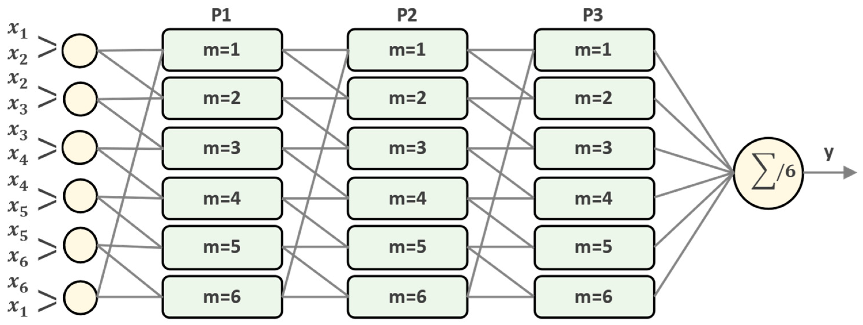
In the above equation $u_k={\displaystyle \prod }_j{F}_{kj}\left(x_j\right)$. $w_k$ denotes the real value of the kth Fuzzy rules [87]. According to the Fuzzy GMDH model, each neuron (partial description) possesses two inputs but one output. As shown in Figure 4, the output vector of each PD in the current layer is the input vector of the following layer. The ultimate output of the Fuzzy GMDH method is determined by averaging the outputs corresponding to the last layer. Therefore, the inputs from the $m_{\mathrm{th}}$ neuron and $p$th layer are taken as the output variables or vectors corresponding to the $m-1$th and $m$th PDs (or neurons) in the $p-1$ layer. Thus, these output vectors are used to generate the input vector (or neuron) in the $m-$th PD (or neuron) and $p$th layer. The relationship in mathematical form between $y^{pm}$, $y^{p-1, m-1}$, and $y^{p-1,m}$ is demonstrated by:

$$y^{pm}=f\left(y^{p-1,m-1},y^{p-1,m}\right)={\displaystyle \sum }_{k=1}^K{\mu }_k^{pm}.w_k^{pm}$$

(29)

${\mu }_k^{pm}$ in the above equation is a mathematical description used for calculating the kth Gaussian function. The following equation ultimately determines the Fuzzy GMDH network output:

$$y=\frac{1}{M}{\displaystyle \sum }_{m=1}^M{y}^{pm}$$

(30)

It should be noted that all the Gaussian functions and weighted coefficients are determined by the trial-and-error method.

Regarding the Fuzzy hybrid GMDH, the backpropagation algorithm must be used to tune all the involved parameters in the PDs and Fuzzy MFs. The problem with this algorithm is that it is unable to determine which PD or link should be eliminated, meaning that the network may contain unnecessary PDs or links. The complex topology of the Fuzzy GMDH model necessitates an efficient algorithm for optimising and tuning Fuzzy MF parameters as well as determining optimal weighting coefficients for PDs in the GMDH algorithm. In this regard, our study employs the HOA algorithm, which has several benefits in exploring and locating the best available solution for highly complex problems [47]. The mentioned algorithm could be used concurrently for network parameter training and structural identification. The HOA algorithm has a number of variables that can be altered to achieve the optimal objective function solution with minimal error. The following function is assumed as the objective function of the optimisation operation in the Fuzzy GMDH based on HOA:

$$Eval=\frac{{{\displaystyle \sum }}_{i=1}^N{\left(y\left(i\right)-\widehat{y}\left(i\right)\right)}^2}{N}$$

(31)

The percentage of the best and worst horses, denoted by pN and qN, respectively. RF (reduction factor), behaviour coefficients for each horse’s age range ($\mathsf{\alpha },\mathsf{\beta },\mathsf{\gamma },\mathsf{\delta }$), number of agents, and maximum number of iterations. Once the process of optimisation is complete, the weighting coefficients are determined. Using the HOA-based Fuzzy GMDH, the Gaussian functions are then derived. In this study, the number of variables and maximum iteration number in the HOA were set to 6 and 150, respectively. In addition, other parameters of the HOA were set similar to [88].

3.6. Statistical Performance

Several performance measures (Equations (32)–(36)) were used in this study, including Wilmot’s Index of Agreement (WI), Root Mean Square Error (RMSE), Correlation Coefficient (CC), Percent Mean Absolute Relative Error (PMARE), and 95% uncertainty (U95).

$$CC=\frac{{{\displaystyle \sum }}_{i=1}^n\left(t_{exp}-\overline{t_{exp}}\right).\left(t_{pre}-\overline{t_{pre}}\right)}{\sqrt{{{\displaystyle \sum }}_{i=1}^n{(t_{exp}-\overline{t_{exp}})}^2{{\displaystyle \sum }}_{i=1}^n{\left(t_{pre}-\overline{t_{pre}}\right)}^2}}$$

(32)

$$RMSE=\sqrt{\frac{1}{n}{{\displaystyle \sum }}_{i=1}^n{\left(t_{pre}-t_{exp}\right)}^2}$$

(33)

$$WI=1-\frac{{{\displaystyle \sum }}_{i=1}^n{\left(t_{exp}-t_{pre}\right)}^2}{{{\displaystyle \sum }}_{i=1}^n{\left(\left|t_{pre}-\overline{t_{exp}}\right|+\left|t_{exp}-\overline{t_{exp}}\right|\right)}^2}$$

(34)

$$PMARE=\frac{100}{n}{{\displaystyle \sum }}_{i=1}^n{\left(t_{pre}-t_{exp}\right)}^2$$

(35)

$$U_{95}=1.96\sqrt{\left(STDE{V}^2+RMS{E}^2\right)}$$

(36)

In the equations mentioned above $t_{exp}$ and $t_{pre}$, respectively, denote the values of experimental and predicted target variables (for example, CS). Additionally, $\overline{t_{exp}}$ and $\overline{t_{pre}}$ represent the mean of experimental and determined target values, respectively. n denotes the total number of the used data. In this study, the RMSE value with the range of (0, +∞) and the optimal value of zero were selected to assess performance. CC measure with the range of (−1 to 1) exhibits the appropriateness of the chosen input variable for determining the target value (with CC ≥ 0.8 being the accepted value), and the PMARE (0, +∞) determines the relative error of measured descriptive and logical behaviours and is based on the relative error. U95 is calculated as the 95% uncertainty band to verify the validity of a model.

4. Application Results and Discussion

The ANFIS, ELM, GMDH, and Fuzzy GMDH-HOA models’ implementation and performance capabilities are examined in this section.

4.1. Implementation of Proposed Models

For the development of the ELM approach, a two-layer architecture was employed. On the basis of prior research [89], the transfer function values, including the sigmoid function, were used to determine the ELM characteristics. To develop the best model’s architecture, 10–120 hidden neuron nodes were proposed. In addition, the RMSE criterion is applied to 500 iterations of the initialisation process for random parameters of hidden layers for each hidden node.

Table 2. Outcomes of the trial-and-error process used to determine the number of neurons in the ELM model.

Model Number	Number of Neurons	RMSE of Training Stage	RMSE of Testing Stage
1	10	10.851	13.524
2	30	9.684	12.289
3	50	9.158	11.235
4	60	7.624	8.362
5	70	7.112	8.027
6	80	6.298	7.899
7	90	5.981	7.389
8	100	6.893	8.068
9	110	7.251	9.621
10	120	8.622	10.136

Best performance is indicated by bold text.

displays the results of the trial-and-error method for determining the optimal number. The 90-neuron ELM model performs best in the learning and validation phases, with less than 6 and 8 % errors, respectively.

In terms of RCDWAC’s standalone ANFIS for CS, the R2019a version of MATLAB software is implemented. In order to create an ANFIS model, an initial Fuzzy inference system must be developed and then trained. The Takagi–Sugeno type’s membership functions (Gaussian MFs) were used for this purpose because they typically produce more robust results [38]. Second, the default hybrid algorithm of ANFIS was used during the training phase, and the least square algorithm was used to set the member function parameters. The optimal architecture of ANFIS for simulation of CS of RCDWAC was determined through a trial-and-error procedure, as shown in

Table 3. Results of the trial-and-error process to determine the number of MFs in the ANFIS model.

Model Number	Number of MFs	RMSE of Training Stage	RMSE of Testing Stage
1	2	9.721	10.189
2	3	7.582	8.428
3	4	6.297	6.317
4	5	6.358	6.581
5	6	5.059	6.554
6	7	4.288	7.263

Best performance is indicated by bold text.

and Figure 5. The ANFIS predictive model was developed using six predictors and four MFs for each input variable with 100 iterations to estimate the compressive strength of RCDWAC based on this structure.

In this study, based on MATLAB open-source code for GMDH evaluation, randomised data information is separated into a calibration subset and a validation subset in order to present new predictive models of CS of RCDWAC. The calibrating subset is utilised in the method’s learning process. The validating phase is used to determine the predictive technique’s performance capacity. Consequently, the GMDH model was implemented using six quadratic polynomials neurons based on a trial-and-error approach to reduce the measurement of each neuron [87].

The developed Fuzzy GMDH-HOA is implemented by the metaheuristic optimisation algorithm. The proposed model was included in partial description which is based on Gaussian variables and the Fuzzy rule and weights. The HOA algorithm was performed for optimising crucial parameters in PDs. Operation of the coupling and optimising process of the neuro-Fuzzy approach and HOA is a parallel interaction in each PD (neurons). As mentioned before, the proposed Fuzzy GMDH-HOA model for CS of RCDWAC has six independent predictors. Developed Fuzzy GMDH-HOA was implemented in the architecture of two Fuzzy rules and six weighting coefficients.

4.2. A Comparison of Models

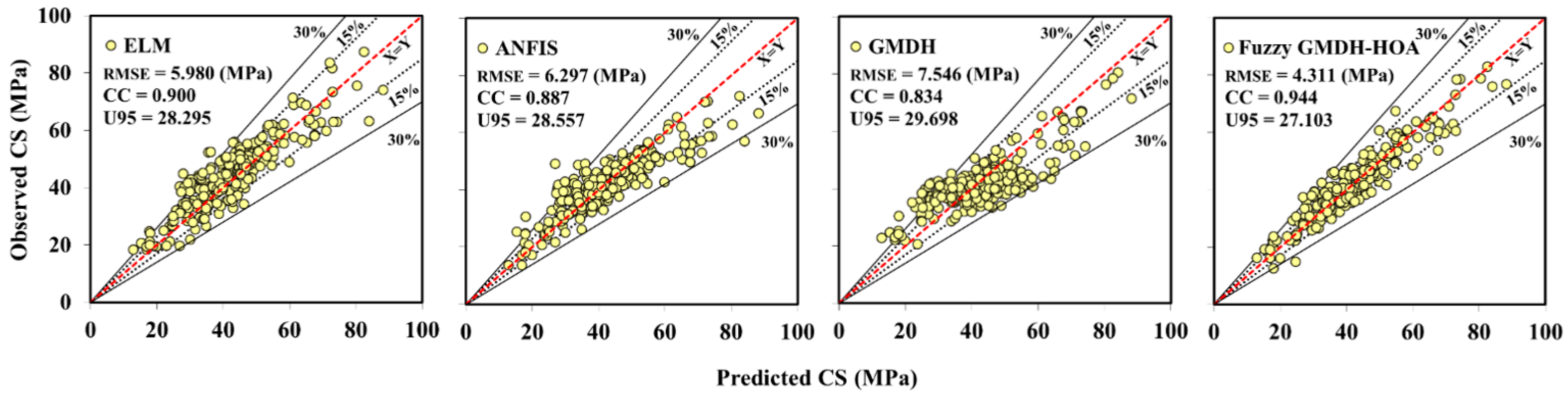
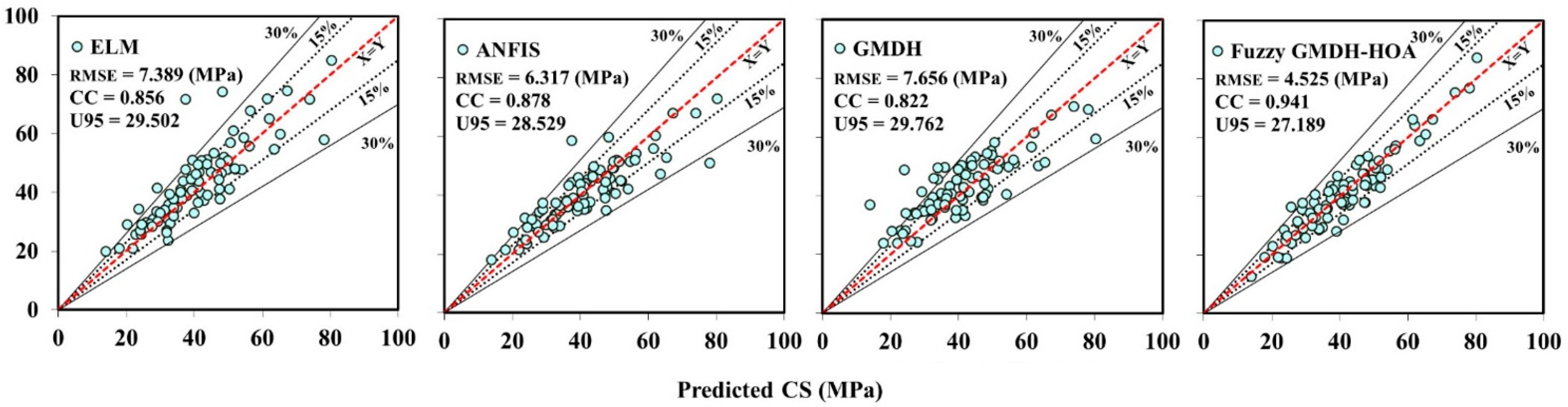
The applicability of the regression-based AI method (e.g., GMDH, ANFIS, ELM, and novel proposed Fuzzy GMDH-HOA) was studied to evaluate the compressive strength of RCDWAC. The performance capability metrics of the developed AI method for the evaluation of concrete behaviour strength are presented in

Table 4. Performance of predictive models.

Performance	Models	CC	RMSE (MPa)	PMARE (%)	U95	WI
Training subset	GMDH	0.834	7.546	15.925	29.698	0.876
	ANFIS	0.887	6.297	10.639	28.557	0.922
	Fuzzy GMDH-HOA	0.944	4.311	8.3182	27.103	0.970
	ELM	0.900	5.980	12.326	28.295	0.942
Testing subset	GMDH	0.822	7.656	17.063	29.762	0.884
	ANFIS	0.878	6.317	10.864	28.529	0.926
	Fuzzy GMDH-HOA	0.941	4.525	9.551	27.189	0.969
	ELM	0.856	7.389	13.638	29.502	0.918
	Gholampour, Gandomi and Ozbakkaloglu [42]	0.756	10.703	26.926	33.177	0.790
	Abdollahzadeh, Jahani and Kashir [49]	−0.150	16.129	31.645	40.743	0.322
	209-Creep and Concrete [48]	0.531	20.192	38.605	47.190	0.555

Best performance is indicated by bold text.

.

In this research, based on a 75–25% data dividing feature, the proposed hybridised and self-adaptive Fuzzy GMDH-HOA model (CC = 0.944, RMSE = 4.311 MPa and U95 = 27.103) and (CC = 0.941. RMSE = 4.525 MPa and U95 = 27.189), outperformed the other regression-based AI techniques and experimental equations in both calibrating (train) and validating (test) phases, respectively. For further investigation of the Fuzzy GMDH-HOA model, predictive equations extracted from the aforementioned method attained the lowest value of PMARE (9.551%) and highest value of WI (0.969); it indicated that hybridising of the AI method enhanced the accuracy of calibrating and validating the subset in terms of WI of the GMDH, ANFIS, and ELM by 8.5%, 4.1%, and 5.1%, respectively.

The validation measures through the regression slope (external validation) [90] for estimation of CS of RCDWAC using the presented models are reported in

Table 5. External validation of predictive models.

Models	K	KPRIME	M	N	RM
GMDH	0.964	1.005	−0.441	−0.477	0.306
NF	1.020	0.958	−0.288	−0.272	0.407
Fuzzy GMDH-HOA	1.005	0.983	−0.128	−0.124	0.587
ELM	0.942	1.033	−0.311	−0.345	0.382
Equation	$\frac{t_{exp}\times t_{pre}}{t_{exp}^2}$	$\frac{R^2-R_0^2}{R^2}$	$\frac{R^2-{R_0^{\prime }}^2}{R^2}$		$R^2\times \left(1-\sqrt{\left|R^2-R_0^2\right|}\right)$
	$\mathrm{Where}\hspace{1em}\hspace{1em}\hspace{1em}\begin{array}{c}{R}_0^2=1-{\displaystyle \sum }_{i=1}^n{t}_{pre}^2{\left(1-k\right)}^2/{\displaystyle \sum }_{i=1}^n{t}_{pre}-\overline{t_{pre}}{)}^2\\ {R_0^{\prime }}^2=1-{\displaystyle \sum }_{i=1}^n{t}_{exp}^2{\left(1-k^{\prime }\right)}^2/{\displaystyle \sum }_{i=1}^n{t}_{exp}-\overline{t_{exp}}{)}^2\end{array}$
Condition	(0.85 < K and Kprim < 1.15)		(m and n < 0.1)		(Rm > 0.5)

. Based on the table, Fuzzy GMDH-HOA with K^prim of 0.983, n of −0.124, and $R_m$ of 0.587 satisfies the required conditions with the best validation compared to those yielded by other methods such as GMDH (K^prim = 1.005, n = −0.477), ANFIS (K^prim = 0.958, n = −0.272), and ELM (K^prim = 0.942, n = −0.345) models. Moreover, the values of $R_m$ for GMDH ($R_m$ = 0.306), ANFIS ($R_m$ = 0.407), and ELM ($R_m$ = 0.382) were lower than the recommended condition ($R_m>$ 0.5). Therefore, Fuzzy GMDH-HOA was based on an optimistic CS estimation model, and computational correlations were not randomly determined.

Moreover, in this study,

Table 6. Summary of the previous studies on prediction models of recycled concrete.

Reference	Method	CC	RMSE	Range of CS	Age of Sample	Sample Size	Number of Input Parameters
Present study	Fuzzy GMDH-HOA	0.94	4.525	13–88	7, 28, 56, 90, 180	353	6
Ahmad, Chaiyasarn, Farooq, Ahmad, Suparp, and Aslam [92]	ANN	0.97	4.36	20–108	7, 28, 90, 180	344	9
	GEP	0.96	3.05
Salimbahrami and Shakeri [93]	ANN	0.97	15.02	18–60	7, 28	124	7
	SVM	0.98	14.97
	MLR	0.81	15.99
Yuan, Tian, Ahmad, Ahmad, Usanova, Mohamed, and Khallaf [91]	GB	0.81	6.976	17–103		638	12
	RF	0.84	5.642
Naderpour et al. [94]	ANN	0.82	6.116	9.85–80.52	28	139	6

is provided in order to discuss the outcomes of the present study with other ones in terms of four aforementioned factors. It is found that the accuracy of the current model seems to provide accurate and precise results in comparison to the previous studies while the number of sample sizes of the current model is much larger than those in the past, except Yuan et al. [91] that used 638 datasets for model development. However, it can be seen from the results of Yuan, Tian, Ahmad, Ahmad, Usanova, Mohamed, and Khallaf [91] that the accuracy of the models compared to the present research decreased significantly by about 15 and 32% in terms of CC and RMSE, respectively. Results from Ahmad et al. [92] are similar and slightly more accurate than the present study because of two important factors: (1) number of input parameters; and (2) number of datasets. It is proven that in many cases having more input variables can improve the accuracy of the models and increase the complexity of the models. The comparison indicated that the current model with fewer input variables and comprehensive datasets is sufficient for predicting the recycled concrete strength.

In addition, regarding to comparison of the model prediction with empirical dataset, it should be noted that in the first step of model development, the network of each model is trained and constructed, and the network then evaluated using unseen datasets called the testing step as the second step. Therefore, assessing the proposed models in the identified range of the dataset will lead to similar prediction results.

Figure 6 and Figure 7 display scatterplots for a graphical comparison of AI models based on regression. Fuzzy GMDH-HOA has the highest correlation around the X = Y ideal line during the calibrating and validating phases. In light of these numbers, the CS values calculated using the proposed Fuzzy GMDH and HOA are approximately closest to the perfect line.

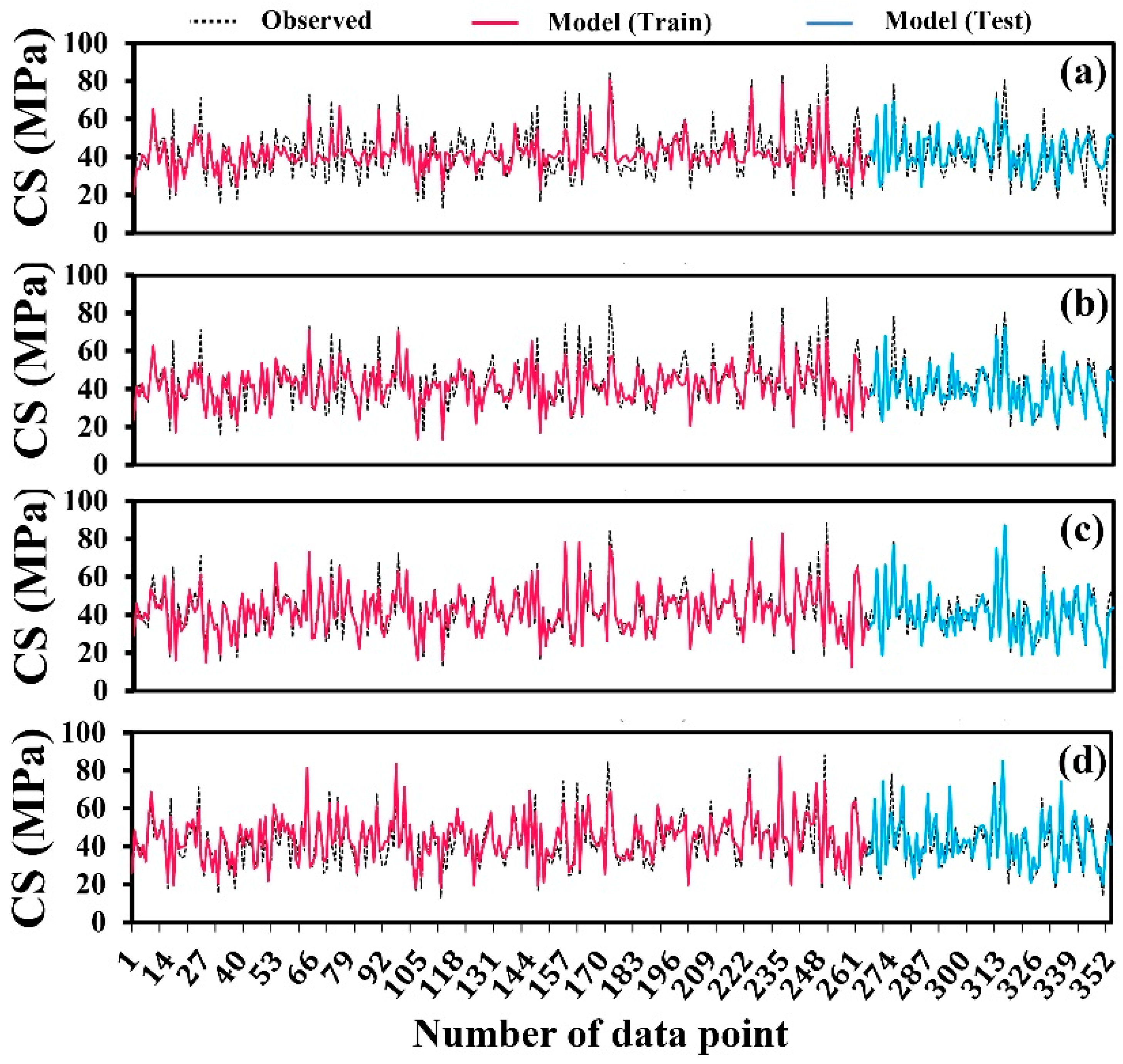
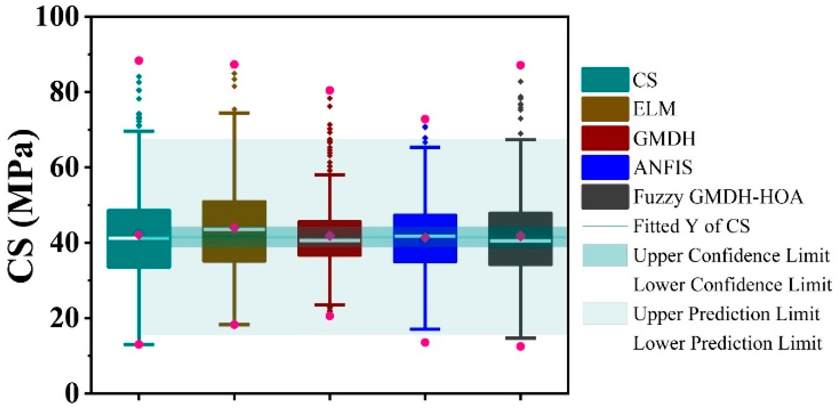
Figure 8 depicts the time series plot for evaluating CS experimental data records (black and dashed line) and proposed data-driven models (coloured and solid line). The Fuzzy GMDH-HOA improved the estimation accuracy of the local maximum (in the range of 50–80 MPa) and minimum values of RCDWAC strengths over other AI tools. A boxplot of the absolute error with quartile values was created for AI analysis (Figure 9). The boxplot’s lower, upper, and middle lines represent the first quartile, third quartile, and median values, respectively. The Fuzzy GMDH-HOA model median and whiskers for simulated and actual CS were nearly identical. The Fuzzy GMDH-HOA model achieved significantly greater statistical precision than the other AI tools.

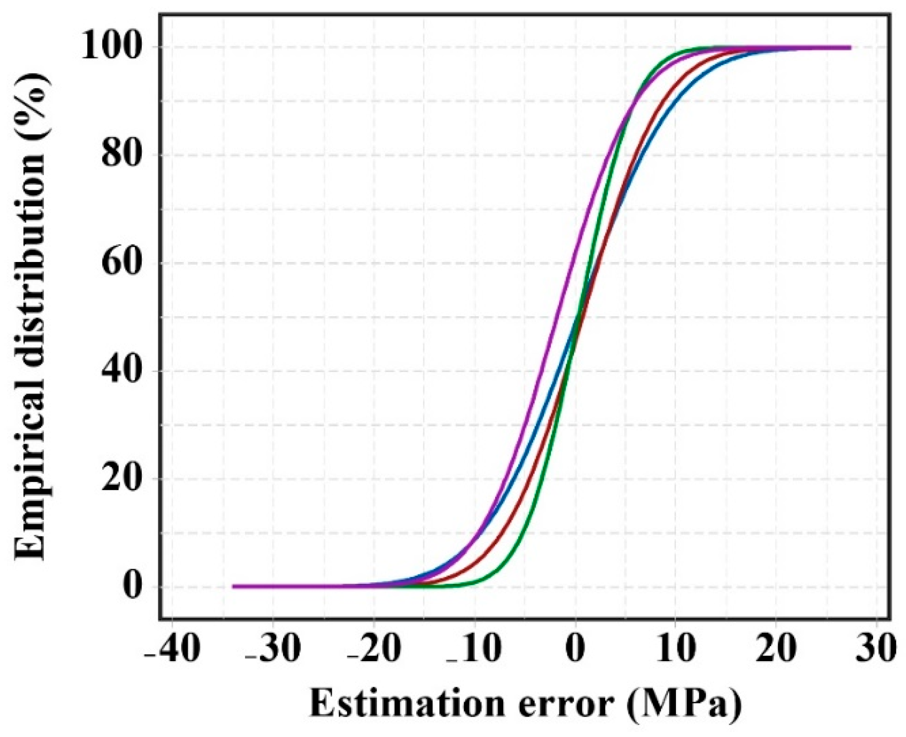
In addition, the Empirical Cumulative Distribution Function (ECDF) analysis was used to measure and investigate the percentage form of the estimated statistical error (|CS|) for the proposed regression-based AI approaches (Figure 10). Concerning the percentage of errors presented within the estimation error range (i.e., from −34.102 to 27.402 MPa), the ECDF reported the capability of Fuzzy GMDH-HOA for estimating the CS of RCDWAC.

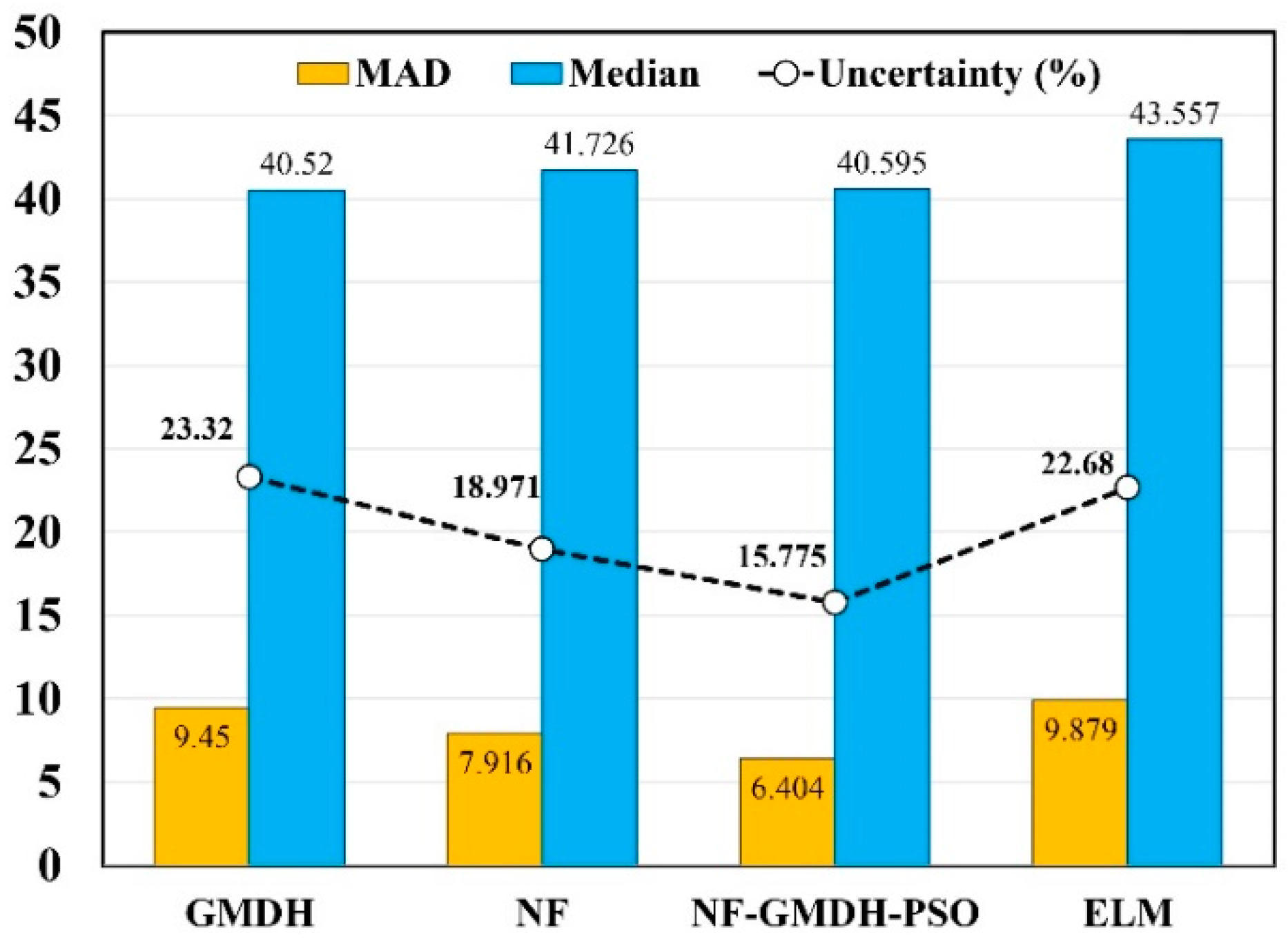
The Monte-Carlo Simulation (MCS) method is used to model uncertainty and specify randomness in a model. Based on probabilistic events, the military was the first to implement MCS [95,96,97]. Predicting the CS involves numerous uncertainties and difficulties, such as the uncertainties associated with input predictors, the uncertainties related to model parameters, etc. The MCS is utilised with forecasting models GMDH, ANFIS, ELM, and GMDH HOA that utilise CS values. Figure 11 displays the results of this study, including the Mean Absolute Deviation (MAD), median of predicted CS, and uncertainty bandwidth. According to the figure, the positive values obtained for the mean of the estimation error indicating that the estimated CS through the application of the predictive models is greater than those obtained through experimentation. In addition, the lower (15.775 percent) and higher (23.320 percent) uncertainty bands were produced by the Fuzzy GMDH-HOA and GMDH, respectively.

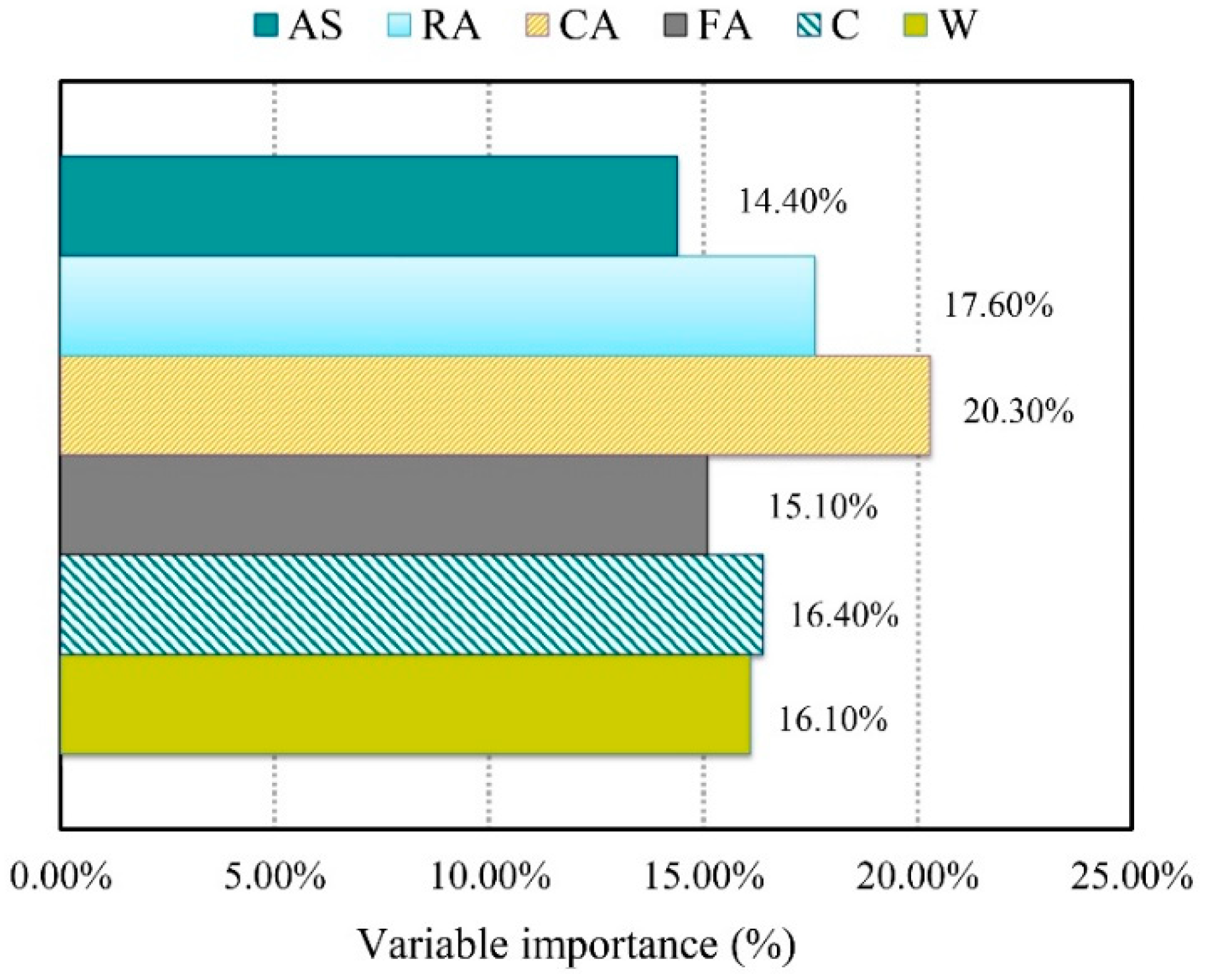
4.3. Variable Importance Analysis

Variable Importance (VA) analysis determines how differences in the values of independent variables affect the dependent variable. The VA percentage is denoted as follows for each model’s inputs [88]:

$$L_i=t_{max}\left(x_i\right)-t_{min}\left(x_i\right)$$

(37)

$$V{A}_i=\frac{L_i}{{{\displaystyle \sum }}_{j=1}^M{L}_i}\times 100$$

(38)

where $t_{max}$ and $t_{min}$ are the maximum and minimum values of the simulated CS over the ith input domain and other predictor values are equal to their mean values. Using the Fuzzy GMDH-HOA model, Figure 12 depicts the outcome of VA analysis for RCDWAC CS evaluation based on the Fuzzy GMDH-HOA model (optimistic developed model). This figure indicated that the coarse aggregate (20.03% importance) content is the most influential independent predictor in CS of RCDWAC.

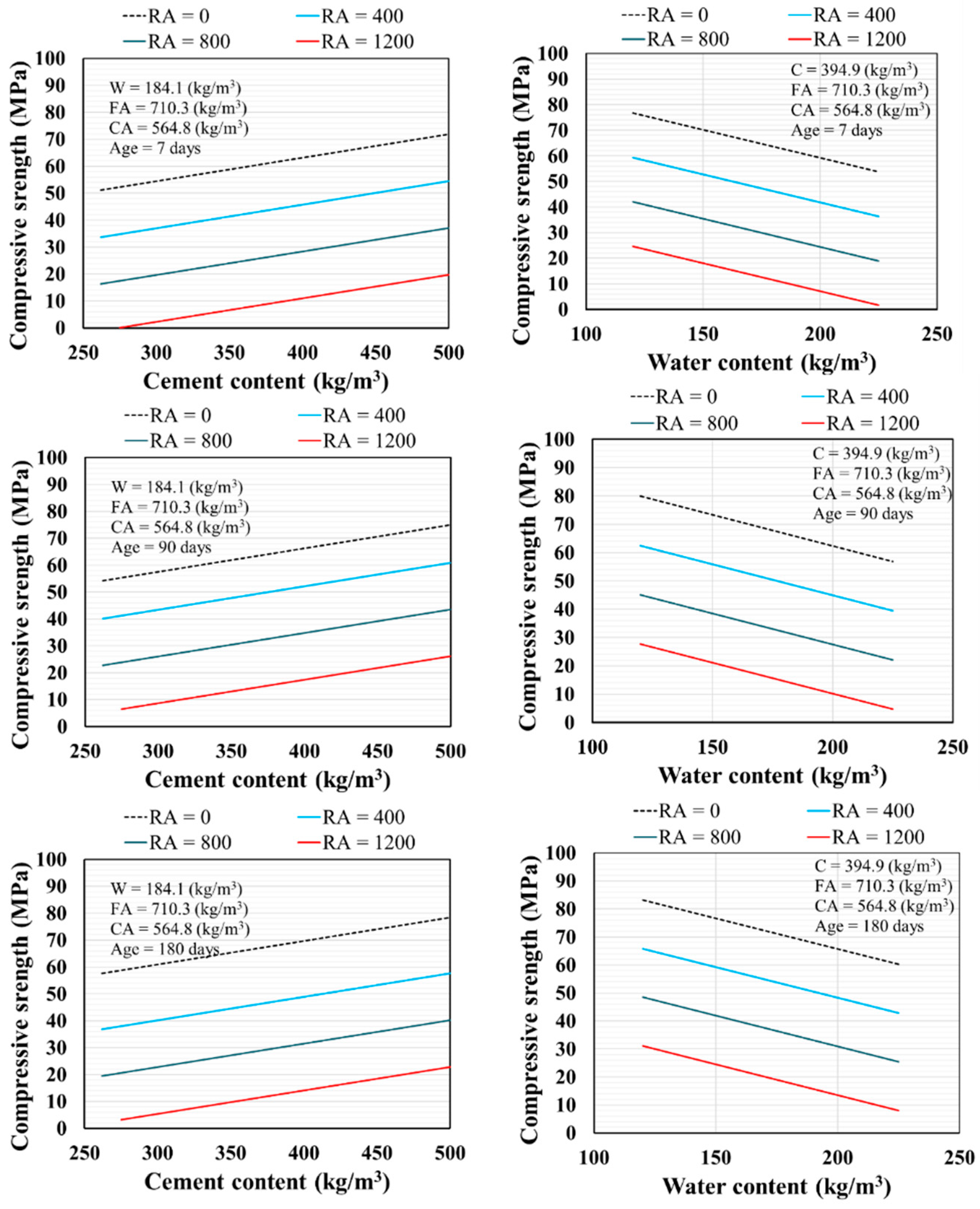
4.4. Parametric Evaluation of RCDWA on CS

A parametric study was applied to evaluate the presented evolutionary Fuzzy GMDH-HOA model based on experimentally effective constituents (e.g., RA, CA, FA, C, W, and AS). The model’s compatibility between estimated values and RCDWAC mixtures was evaluated to determine the quality and validity of the developed Fuzzy-based design model. In this study, only selected input variables are treated as variables at any given time, while other experimental factors are treated as constants based on the mean values of their entire datasets [55]. Mechanical properties of RCDWAC mixtures are highly dependent on the mix design and the materials used, and even small changes in the composition of materials can have significant effects. The projects constructed with the optimal content produced a more uniform mixture and, as a result, enhanced mechanical properties. Overall, the model accurately predicts all trends with smooth curves. Specifically, Figure 13 depicted the expected decrease in CS values with the use of water content in recycled aggregates with long and short curing times (7, 90, and 180 days), as well as the fact that excessive water content in recycled aggregates may cause segregation problems.

5. Summary and Conclusions

Recycled Construction and Demolition Waste Aggregate Concrete (RCDWAC) is an eco-friendly and cost-effective alternative to conventional concrete in the construction industry. This study aimed to implement an eco-friendly solution based on a novel Artificial Intelligence (AI) method in concrete technology for modelling and estimating the Compressive Strength (CS) of RCDWAC using an alternative artificial computing system known as Fuzzy GMDH-HOA. Several AI benchmark methods, such as the supervised learning method (e.g., GMDH), Fuzzy paradigm (e.g., the NeuroFuzzy system), and committee-based model, were compared with the presented model to determine its efficacy and capability (e.g., ELM). In addition, the uncertainty of the presented novel Fuzzy GMDH-HOA model was investigated using the Monte-Carlo simulation framework. For evaluating the predictability of the developed models, statistical indicators including PMARE, CC, U95, RMSE, and WI were utilised. In this regard, the RMSE and PMARE values of the Fuzzy-GMDH-HOA model for CS prediction were decreased to 30.8% and 7.5%, respectively, when compared to the standalone GMDH model. This study’s findings demonstrated the predictive capacity of the proposed Fuzzy GMDH-HOA in developing a reasonable and robust regression-based AI technique for predicting the CS of RCDWAC. On the basis of AI computational operation, modelling error, and visual consideration (e.g., scatterplots, time series plots, boxplot, and ECDF distribution diagram), the proposed model extracted from Fuzzy GMDH can improve accuracy by hybridising the evolutionary HOA algorithm. According to a sensitivity analysis, the coarse aggregate is the most influential independent variable in RCDWAC mix design, accounting for 20.03% of its importance.

Nonetheless, this paper proposed an innovative hybridisation of evolutionary models to evaluate the CS of RCDWAC; future research should address several limitations. As suggested by hybridised computation, Fuzzy GMDH-HOA may be used to simulate the CS of RCDWAC with a high level of estimation capability. One of the disadvantages of the proposed Fuzzy GMDH-HOA is that the technique is time-consuming because tuning parameters are used to achieve optimal conditions. To circumvent these limitations, it was determined that more metaheuristic optimisation algorithms with a high level of convergence should be utilised. More focus should be placed on coupling AI, and the data mining approach (ensemble mechanism, deep learning methods, etc.) could be extended to include the data mining approach. As can be presented from the AI process, the proposed model could predict the CS of RCDWAC in different input types with optimal performance. One of the disadvantages of the proposed hybrid model (e.g., Fuzzy-GMDH-HOA) is that non-equation-based prediction and its implementation is time-consuming because it optimized user manual parameters of the model. Therefore, it was recommended to propose more evolutionary AI approaches for domination of these limitations via high convergence speed algorithms, classifiers, and methods. More focus should be placed on coupling AI, and data mining approaches (ensemble mechanism, deep learning methods, etc.) could be extended to include the data mining approach.

References

1. Yazdani, M.; Mojtahedi, M.; Loosemore, M. Enhancing evacuation response to extreme weather disasters using public transportation systems: A novel simheuristic approach. J. Comput. Des. Eng. 2020, 7, 195–210. [Google Scholar] [CrossRef]
2. Yazdani, M.; Mojtahedi, M.; Loosemore, M.; Sanderson, D. A modelling framework to design an evacuation support system for healthcare infrastructures in response to major flood events. Prog. Disaster Sci. 2022, 13, 100218. [Google Scholar] [CrossRef]
3. Wei, W.; Mojtahedi, M.; Yazdani, M.; Kabirifar, K. The Alignment of Australia’s National Construction Code and the Sendai Framework for Disaster Risk Reduction in Achieving Resilient Buildings and Communities. Buildings 2021, 11, 429. [Google Scholar] [CrossRef]
4. Shahmansouri, A.A.; Yazdani, M.; Hosseini, M.; Bengar, H.A.; Ghatte, H.F. The prediction analysis of compressive strength and electrical resistivity of environmentally friendly concrete incorporating natural zeolite using artificial neural network. Constr. Build. Mater. 2022, 317, 125876. [Google Scholar] [CrossRef]
5. Kabirifar, K.; Mojtahedi, M.; Changxin Wang, C.; Tam, V.W.Y. Effective construction and demolition waste management assessment through waste management hierarchy; a case of Australian large construction companies. J. Clean. Prod. 2021, 312, 127790. [Google Scholar] [CrossRef]
6. Mirmozaffari, M.; Yazdani, M.; Boskabadi, A.; Ahady Dolatsara, H.; Kabirifar, K.; Amiri Golilarz, N. A novel machine learning approach combined with optimization models for eco-efficiency evaluation. Appl. Sci. 2020, 10, 5210. [Google Scholar] [CrossRef]
7. Yazdani, M.; Kabirifar, K.; Frimpong, B.E.; Shariati, M.; Mirmozaffari, M.; Boskabadi, A. Improving construction and demolition waste collection service in an urban area using a simheuristic approach: A case study in Sydney, Australia. J. Clean. Prod. 2021, 280, 124138. [Google Scholar] [CrossRef]
8. Akbarzadeh Bengar, H.; Shahmansouri, A.A.; Akkas Zangebari Sabet, N.; Kabirifar, K.; Tam, V.W. Impact of elevated temperatures on the structural performance of recycled rubber concrete: Experimental and mathematical modeling. Constr. Build. Mater. 2020, 255, 119374. [Google Scholar] [CrossRef]
9. Ghafourian, K.; Kabirifar, K.; Mahdiyar, A.; Yazdani, M.; Ismail, S.; Tam, V.W. A synthesis of express analytic hierarchy process (EAHP) and partial least squares-structural equations modeling (PLS-SEM) for sustainable construction and demolition waste management assessment: The case of Malaysia. Recycling 2021, 6, 73. [Google Scholar] [CrossRef]
10. Abera, Y.A. Performance of concrete materials containing recycled aggregate from construction and demolition waste. Results Mater. 2022, 14, 100278. [Google Scholar] [CrossRef]
11. Akhtar, A.; Sarmah, A.K. Construction and demolition waste generation and properties of recycled aggregate concrete: A global perspective. J. Clean. Prod. 2018, 186, 262–281. [Google Scholar] [CrossRef]
12. de Andrade Salgado, F.; de Andrade Silva, F. Recycled aggregates from construction and demolition waste towards an application on structural concrete: A review. J. Build. Eng. 2022, 52, 104452. [Google Scholar] [CrossRef]
13. Özalp, F.; Yılmaz, H.D.; Kara, M.; Kaya, Ö.; Şahin, A. Effects of recycled aggregates from construction and demolition wastes on mechanical and permeability properties of paving stone, kerb and concrete pipes. Constr. Build. Mater. 2016, 110, 17–23. [Google Scholar] [CrossRef]
14. del Bosque, I.S.; Van den Heede, P.; De Belie, N.; De Rojas, M.S.; Medina, C. Carbonation of concrete with construction and demolition waste based recycled aggregates and cement with recycled content. Constr. Build. Mater. 2020, 234, 117336. [Google Scholar] [CrossRef]
15. Bui, N.K.; Satomi, T.; Takahashi, H. Improvement of mechanical properties of recycled aggregate concrete basing on a new combination method between recycled aggregate and natural aggregate. Constr. Build. Mater. 2017, 148, 376–385. [Google Scholar] [CrossRef]
16. Kabirifar, K.; Mojtahedi, M.; Wang, C.; Tam, V.W.Y. Construction and demolition waste management contributing factors coupled with reduce, reuse, and recycle strategies for effective waste management: A review. J. Clean. Prod. 2020, 263, 121265. [Google Scholar] [CrossRef]
17. Ann, K.Y.; Moon, H.; Kim, Y.; Ryou, J. Durability of recycled aggregate concrete using pozzolanic materials. Waste Manag. 2008, 28, 993–999. [Google Scholar] [CrossRef]
18. Ghanbari, S.; Shahmansouri, A.A.; Akbarzadeh Bengar, H.; Jafari, A. Compressive strength prediction of high-strength oil palm shell lightweight aggregate concrete using machine learning methods. Environ. Sci. Pollut. Res. 2022, 1–20. [Google Scholar] [CrossRef]
19. Mehrabi, P.; Shariati, M.; Kabirifar, K.; Jarrah, M.; Rasekh, H.; Trung, N.T.; Shariati, A.; Jahandari, S. Effect of pumice powder and nano-clay on the strength and permeability of fiber-reinforced pervious concrete incorporating recycled concrete aggregate. Constr. Build. Mater. 2021, 287, 122652. [Google Scholar] [CrossRef]
20. Shahmansouri, A.A.; Yazdani, M.; Ghanbari, S.; Bengar, H.A.; Jafari, A.; Ghatte, H.F. Artificial neural network model to predict the compressive strength of eco-friendly geopolymer concrete incorporating silica fume and natural zeolite. J. Clean. Prod. 2021, 279, 123697. [Google Scholar] [CrossRef]
21. AzariJafari, H.; Taheri Amiri, M.J.; Ashrafian, A.; Rasekh, H.; Barforooshi, M.J.; Berenjian, J. Ternary blended cement: An eco-friendly alternative to improve resistivity of high-performance self-consolidating concrete against elevated temperature. J. Clean. Prod. 2019, 223, 575–586. [Google Scholar] [CrossRef]
22. Shahmansouri, A.A.; Akbarzadeh Bengar, H.; Ghanbari, S. Compressive strength prediction of eco-efficient GGBS-based geopolymer concrete using GEP method. J. Build. Eng. 2020, 31, 101326. [Google Scholar] [CrossRef]
23. Ashrafian, A.; Gandomi, A.H.; Rezaie-Balf, M.; Emadi, M. An evolutionary approach to formulate the compressive strength of roller compacted concrete pavement. Measurement 2020, 152, 107309. [Google Scholar] [CrossRef]
24. Ashrafian, A.; Taheri Amiri, M.J.; Rezaie-Balf, M.; Ozbakkaloglu, T.; Lotfi-Omran, O. Prediction of compressive strength and ultrasonic pulse velocity of fiber reinforced concrete incorporating nano silica using heuristic regression methods. Constr. Build. Mater. 2018, 190, 479–494. [Google Scholar] [CrossRef]
25. Asteris, P.G.; Ashrafian, A.; Rezaie-Balf, M. Prediction of the compressive strength of self-compacting concrete using surrogate models. Comput. Concr 2019, 24, 137–150. [Google Scholar]
26. NoParast, M.; Hematian, M.; Ashrafian, A.; Amiri, M.J.T.; AzariJafari, H. Development of a non-dominated sorting genetic algorithm for implementing circular economy strategies in the concrete industry. Sustain. Prod. Consum. 2021, 27, 933–946. [Google Scholar] [CrossRef]
27. Taheri Amiri, M.J.; Ashrafian, A.; Haghighi, F.R.; Javaheri Barforooshi, M. Prediction of the compressive strength of self-compacting concrete containing rice husk ash using data driven models. Modares Civ. Eng. J. 2019, 19, 209–221. [Google Scholar]
28. Ashrafian, A.; Taheri Amiri, M.J.; Haghighi, F. Modeling the slump flow of self-compacting concrete incorporating Metakaolin using soft computing techniques. J. Struct. Constr. Eng. 2019, 6, 5–20. [Google Scholar]
29. Ashrafian, A.; Taheri Amiri, M.J.; Masoumi, P.; Asadi-shiadeh, M.; Yaghoubi-chenari, M.; Mosavi, A.; Nabipour, N. Classification-based regression models for prediction of the mechanical properties of roller-compacted concrete pavement. Appl. Sci. 2020, 10, 3707. [Google Scholar] [CrossRef]
30. Rezaie-Balf, M.; Maleki, N.; Kim, S.; Ashrafian, A.; Babaie-Miri, F.; Kim, N.W.; Chung, I.-M.; Alaghmand, S. Forecasting daily solar radiation using CEEMDAN decomposition-based MARS model trained by crow search algorithm. Energies 2019, 12, 1416. [Google Scholar] [CrossRef] [Green Version]
31. Sadowski, Ł.; Piechówka-Mielnik, M.; Widziszowski, T.; Gardynik, A.; Mackiewicz, S. Hybrid ultrasonic-neural prediction of the compressive strength of environmentally friendly concrete screeds with high volume of waste quartz mineral dust. J. Clean. Prod. 2019, 212, 727–740. [Google Scholar] [CrossRef]
32. DeRousseau, M.A.; Laftchiev, E.; Kasprzyk, J.R.; Rajagopalan, B.; Srubar, W.V. A comparison of machine learning methods for predicting the compressive strength of field-placed concrete. Constr. Build. Mater. 2019, 228, 116661. [Google Scholar] [CrossRef]
33. Shahmansouri, A.A.; Akbarzadeh Bengar, H.; Jahani, E. Predicting compressive strength and electrical resistivity of eco-friendly concrete containing natural zeolite via GEP algorithm. Constr. Build. Mater. 2019, 229, 116883. [Google Scholar] [CrossRef]
34. Ashrafian, A.; Shokri, F.; Taheri Amiri, M.J.; Yaseen, Z.M.; Rezaie-Balf, M. Compressive strength of Foamed Cellular Lightweight Concrete simulation: New development of hybrid artificial intelligence model. Constr. Build. Mater. 2020, 230, 117048. [Google Scholar] [CrossRef]
35. Naseri, H.; Jahanbakhsh, H.; Hosseini, P.; Moghadas Nejad, F. Designing sustainable concrete mixture by developing a new machine learning technique. J. Clean. Prod. 2020, 258, 120578. [Google Scholar] [CrossRef]
36. Dao, D.V.; Ly, H.-B.; Trinh, S.H.; Le, T.-T.; Pham, B.T. Artificial Intelligence Approaches for Prediction of Compressive Strength of Geopolymer Concrete. Materials 2019, 12, 983. [Google Scholar] [CrossRef] [Green Version]
37. Asteris, P.G.; Mokos, V.G. Concrete compressive strength using artificial neural networks. Neural Comput. Appl. 2020, 32, 11807–11826. [Google Scholar] [CrossRef]
38. Golafshani, E.M.; Behnood, A.; Arashpour, M. Predicting the compressive strength of normal and High-Performance Concretes using ANN and ANFIS hybridized with Grey Wolf Optimizer. Constr. Build. Mater. 2020, 232, 117266. [Google Scholar] [CrossRef]
39. Behnood, A.; Golafshani, E.M. Machine learning study of the mechanical properties of concretes containing waste foundry sand. Constr. Build. Mater. 2020, 243, 118152. [Google Scholar] [CrossRef]
40. Feng, D.-C.; Liu, Z.-T.; Wang, X.-D.; Chen, Y.; Chang, J.-Q.; Wei, D.-F.; Jiang, Z.-M. Machine learning-based compressive strength prediction for concrete: An adaptive boosting approach. Constr. Build. Mater. 2020, 230, 117000. [Google Scholar] [CrossRef]
41. Li, X.; Khademi, F.; Liu, Y.; Akbari, M.; Wang, C.; Bond, P.L.; Keller, J.; Jiang, G. Evaluation of data-driven models for predicting the service life of concrete sewer pipes subjected to corrosion. J. Environ. Manag. 2019, 234, 431–439. [Google Scholar] [CrossRef] [PubMed]
42. Gholampour, A.; Gandomi, A.H.; Ozbakkaloglu, T. New formulations for mechanical properties of recycled aggregate concrete using gene expression programming. Constr. Build. Mater. 2017, 130, 122–145. [Google Scholar] [CrossRef]
43. Al-Shamiri, A.K.; Kim, J.H.; Yuan, T.-F.; Yoon, Y.S. Modeling the compressive strength of high-strength concrete: An extreme learning approach. Constr. Build. Mater. 2019, 208, 204–219. [Google Scholar] [CrossRef]
44. Precup, R.-E.; David, R.-C. Nature-Inspired Optimization Algorithms for Fuzzy Controlled Servo Systems; Butterworth-Heinemann: Oxford, UK, 2019. [Google Scholar]
45. Wong, W.K.; Guo, Z.X.; Leung, S. Optimizing Decision Making in the Apparel Supply Chain Using Artificial Intelligence (AI): From Production to Retail; Elsevier: Amsterdam, The Netherlands, 2013. [Google Scholar]
46. Imran, M.; Alsuhaibani, S.A. A neuro-fuzzy inference model for diabetic retinopathy classification. In Intelligent Data Analysis for Biomedical Applications; Elsevier: Amsterdam, The Netherlands, 2019; pp. 147–172. [Google Scholar]
47. MiarNaeimi, F.; Azizyan, G.; Rashki, M. Horse herd optimization algorithm: A nature-inspired algorithm for high-dimensional optimization problems. Knowl.-Based Syst. 2021, 213, 106711. [Google Scholar] [CrossRef]
48. ACI Committee 209-Creep and Volume Changes in Concrete. Prediction of Creep, Shrinkage, and Temperature Effects in Concrete Structures; American Concrete Institute: Farmington Hills, MI, USA, 1982. [Google Scholar]
49. Abdollahzadeh, G.; Jahani, E.; Kashir, Z. Predicting of compressive strength of recycled aggregate concrete by genetic programming. Comput. Concr. 2016, 18, 155–163. [Google Scholar] [CrossRef]
50. Silva, R.; de Brito, J. Eurocode 2-based structural design of a reinforced recycled aggregate concrete slab. In Proceedings of the UKIERI Concrete Congress, Jalandhar, India, 5–8 March 2019. [Google Scholar]
51. EPA US. United States environmental protection agency. In Quality Assurance Guidance Document-Model Quality Assurance Project Plan for the PM Ambient Air; U.S. Environmental Protection Agency: Washington, DC, USA, 2001; Volume 2. [Google Scholar]
52. Domingo-Cabo, A.; Lázaro, C.; López-Gayarre, F.; Serrano-López, M.A.; Serna, P.; Castaño-Tabares, J.O. Creep and shrinkage of recycled aggregate concrete. Constr. Build. Mater. 2009, 23, 2545–2553. [Google Scholar] [CrossRef]
53. González-Fonteboa, B.; Martínez-Abella, F.; Eiras-López, J.; Seara-Paz, S. Effect of recycled coarse aggregate on damage of recycled concrete. Mater. Struct. 2011, 44, 1759. [Google Scholar] [CrossRef]
54. Casuccio, M.; Torrijos, M.C.; Giaccio, G.; Zerbino, R. Failure mechanism of recycled aggregate concrete. Constr. Build. Mater. 2008, 22, 1500–1506. [Google Scholar] [CrossRef]
55. Zega, C.J.; Di Maio, A.A. Recycled concrete made with different natural coarse aggregates exposed to high temperature. Constr. Build. Mater. 2009, 23, 2047–2052. [Google Scholar] [CrossRef]
56. Thomas, J.; Thaickavil, N.N.; Wilson, P.M. Strength and durability of concrete containing recycled concrete aggregates. J. Build. Eng. 2018, 19, 349–365. [Google Scholar] [CrossRef]
57. Folino, P.; Xargay, H. Recycled aggregate concrete—Mechanical behavior under uniaxial and triaxial compression. Constr. Build. Mater. 2014, 56, 21–31. [Google Scholar] [CrossRef]
58. Duan, Z.H.; Poon, C.S. Properties of recycled aggregate concrete made with recycled aggregates with different amounts of old adhered mortars. Mater. Des. 2014, 58, 19–29. [Google Scholar] [CrossRef]
59. Vieira, J.P.B.; Correia, J.R.; de Brito, J. Post-fire residual mechanical properties of concrete made with recycled concrete coarse aggregates. Cem. Concr. Res. 2011, 41, 533–541. [Google Scholar] [CrossRef]
60. Zheng, C.; Lou, C.; Du, G.; Li, X.; Liu, Z.; Li, L. Mechanical properties of recycled concrete with demolished waste concrete aggregate and clay brick aggregate. Results Phys. 2018, 9, 1317–1322. [Google Scholar] [CrossRef]
61. Kou, S.-C.; Poon, C.-S. Mechanical properties of 5-year-old concrete prepared with recycled aggregates obtained from three different sources. Mag. Concr. Res. 2008, 60, 57–64. [Google Scholar] [CrossRef]
62. Etxeberria, M.; Vázquez, E.; Marí, A.; Barra, M. Influence of amount of recycled coarse aggregates and production process on properties of recycled aggregate concrete. Cem. Concr. Res. 2007, 37, 735–742. [Google Scholar] [CrossRef]
63. JACOB, L.L.G. Effects of Recycled Aggregates on Concrete Properties. Master’s Thesis, National University of Singapore, Singapore, 2011. [Google Scholar]
64. Chakradhara Rao, M.; Bhattacharyya, S.; Barai, S. Influence of field recycled coarse aggregate on properties of concrete. Mater. Struct. 2011, 44, 205–220. [Google Scholar] [CrossRef]
65. Yang, K.-H.; Chung, H.-S.; Ashour, A.F. Influence of Type and Replacement Level of Recycled Aggregates on Concrete Properties. ACI Mater. J. 2008, 105, 289–296. [Google Scholar]
66. Alengaram, U.J.; Salam, A.; Jumaat, M.Z.; Jaafar, F.F.; Saad, H.B. Properties of high-workability concrete with recycled concrete aggregate. Mater. Res. 2011, 14, 248–255. [Google Scholar]
67. Kotrayothar, D. Recycled Aggregate Concrete for Structural Applications. Ph.D. Thesis, University of Western Sydney Penrith Campus, Kingswood, Australia, 2012. [Google Scholar]
68. Huang, G.-B.; Zhu, Q.-Y.; Siew, C.-K. Extreme learning machine: Theory and applications. Neurocomputing 2006, 70, 489–501. [Google Scholar] [CrossRef]
69. Malekzadeh, M.; Kardar, S.; Shabanlou, S. Simulation of groundwater level using MODFLOW, extreme learning machine and Wavelet-Extreme Learning Machine models. Groundw. Sustain. Dev. 2019, 9, 100279. [Google Scholar] [CrossRef]
70. Shirzadi, A.; Asadi, S.; Shahabi, H.; Ronoud, S.; Clague, J.J.; Khosravi, K.; Pham, B.T.; Ahmad, B.B.; Bui, D.T. A novel ensemble learning based on Bayesian Belief Network coupled with an extreme learning machine for flash flood susceptibility mapping. Eng. Appl. Artif. Intell. 2020, 96, 103971. [Google Scholar] [CrossRef]
71. Valipour, A.; Shirgahi, H. Estimation of rip density on intermediate beaches using an extreme learning machine model. Reg. Stud. Mar. Sci. 2022, 52, 102332. [Google Scholar] [CrossRef]
72. Gharib, Z.; Tavakkoli-Moghaddam, R.; Bozorgi-Amiri, A.; Yazdani, M. Post-Disaster Temporary Shelters Distribution after a Large-Scale Disaster: An Integrated Model. Buildings 2022, 12, 414. [Google Scholar] [CrossRef]
73. Jang, J.S.R. ANFIS: Adaptive-network-based fuzzy inference system. IEEE Trans. Syst. Man Cybern. 1993, 23, 665–685. [Google Scholar] [CrossRef]
74. Kang, F.; Liu, J.; Li, J.; Li, S. Concrete dam deformation prediction model for health monitoring based on extreme learning machine. Struct. Control. Health Monit. 2017, 24, e1997. [Google Scholar] [CrossRef]
75. Kar, S.; Das, S.; Ghosh, P.K. Applications of neuro fuzzy systems: A brief review and future outline. Appl. Soft Comput. 2014, 15, 243–259. [Google Scholar] [CrossRef]
76. Jovic, S.; Smigic Miladinovic, J.; Micic, R.; Markovic, S.; Rakic, G. Analysing of exchange rate and gross domestic product (GDP) by adaptive neuro fuzzy inference system (ANFIS). Phys. A Stat. Mech. Appl. 2019, 513, 333–338. [Google Scholar] [CrossRef]
77. Shiri, J.; Kişi, Ö. Comparison of genetic programming with neuro-fuzzy systems for predicting short-term water table depth fluctuations. Comput. Geosci. 2011, 37, 1692–1701. [Google Scholar] [CrossRef]
78. Ivakhnenko, A.G.; Ivakhnenko, G.A. Problems of further development of the group method of data handling algorithms. Part I. Pattern Recognit. Image Anal. C/C Raspoznavaniye Obraz. I Anal. Izobr. 2000, 10, 187–194. [Google Scholar]
79. Amanifard, N.; Nariman-Zadeh, N.; Farahani, M.H.; Khalkhali, A. Modelling of multiple short-length-scale stall cells in an axial compressor using evolved GMDH neural networks. Energy Convers. Manag. 2008, 49, 2588–2594. [Google Scholar] [CrossRef]
80. Ebtehaj, I.; Bonakdari, H.; Gharabaghi, B. Development of more accurate discharge coefficient prediction equations for rectangular side weirs using adaptive neuro-fuzzy inference system and generalized group method of data handling. Measurement 2018, 116, 473–482. [Google Scholar] [CrossRef]
81. Beiki Ashkezari, A.; Zokaee, M.; Aghsami, A.; Jolai, F.; Yazdani, M. Selecting an Appropriate Configuration in a Construction Project Using a Hybrid Multiple Attribute Decision Making and Failure Analysis Methods. Buildings 2022, 12, 643. [Google Scholar] [CrossRef]
82. Safaeian, M.; Fathollahi-Fard, A.M.; Kabirifar, K.; Yazdani, M.; Shapouri, M. Selecting Appropriate Risk Response Strategies Considering Utility Function and Budget Constraints: A Case Study of a Construction Company in Iran. Buildings 2022, 12, 98. [Google Scholar] [CrossRef]
83. Salari, S.A.-S.; Mahmoudi, H.; Aghsami, A.; Jolai, F.; Jolai, S.; Yazdani, M. Off-Site construction Three-Echelon supply chain management with stochastic constraints: A modelling approach. Buildings 2022, 12, 119. [Google Scholar] [CrossRef]
84. Yazdani, M.; Kabirifar, K.; Fathollahi-Fard, A.M.; Mojtahedi, M. Production scheduling of off-site prefabricated construction components considering sequence dependent due dates. Environ. Sci. Pollut. Res. 2021, 1–17. [Google Scholar] [CrossRef]
85. Yazdani, M.; Jolai, F. Lion optimization algorithm (LOA): A nature-inspired metaheuristic algorithm. J. Comput. Des. Eng. 2016, 3, 24–36. [Google Scholar] [CrossRef] [Green Version]
86. Gharib, Z.; Yazdani, M.; Bozorgi-Amiri, A.; Tavakkoli-Moghaddam, R.; Taghipourian, M.J. Developing an integrated model for planning the delivery of construction materials to post-disaster reconstruction projects. J. Comput. Des. Eng. 2022, 9, 1135–1156. [Google Scholar] [CrossRef]
87. Hwang, H.S. Fuzzy GMDH-type neural network model and its application to forecasting of mobile communication. Comput. Ind. Eng. 2006, 50, 450–457. [Google Scholar] [CrossRef]
88. Ashrafian, A.; Shahmansouri, A.A.; Akbarzadeh Bengar, H.; Behnood, A. Post-fire behavior evaluation of concrete mixtures containing natural zeolite using a novel metaheuristic-based machine learning method. Arch. Civ. Mech. Eng. 2022, 22, 101. [Google Scholar] [CrossRef]
89. Madandoust, R.; Ghavidel, R.; Nariman-zadeh, N. Evolutionary design of generalized GMDH-type neural network for prediction of concrete compressive strength using UPV. Comput. Mater. Sci. 2010, 49, 556–567. [Google Scholar] [CrossRef]
90. Tropsha, A. Best Practices for QSAR Model Development, Validation, and Exploitation. Mol. Inform. 2010, 29, 476–488. [Google Scholar] [CrossRef] [PubMed]
91. Yuan, X.; Tian, Y.; Ahmad, W.; Ahmad, A.; Usanova, K.I.; Mohamed, A.M.; Khallaf, R. Machine Learning Prediction Models to Evaluate the Strength of Recycled Aggregate Concrete. Materials 2022, 15, 2823. [Google Scholar] [CrossRef]
92. Ahmad, A.; Chaiyasarn, K.; Farooq, F.; Ahmad, W.; Suparp, S.; Aslam, F. Compressive strength prediction via gene expression programming (GEP) and artificial neural network (ANN) for concrete containing RCA. Buildings 2021, 11, 324. [Google Scholar] [CrossRef]
93. Salimbahrami, S.R.; Shakeri, R. Experimental investigation and comparative machine-learning prediction of compressive strength of recycled aggregate concrete. Soft Comput. 2021, 25, 919–932. [Google Scholar] [CrossRef]
94. Naderpour, H.; Rafiean, A.H.; Fakharian, P. Compressive strength prediction of environmentally friendly concrete using artificial neural networks. J. Build. Eng. 2018, 16, 213–219. [Google Scholar] [CrossRef]
95. Ashrafian, A.; Panahi, E.; Salehi, S.; Taheri Amiri, M.J. On the implementation of the interpretable data-intelligence model for designing service life of structural concrete in a marine environment. Ocean. Eng. 2022, 256, 111523. [Google Scholar] [CrossRef]
96. Islam, M.S.; Mohandes, S.R.; Mahdiyar, A.; Fallahpour, A.; Olanipekun, A.O. A Coupled Genetic Programming Monte Carlo Simulation–Based Model for Cost Overrun Prediction of Thermal Power Plant Projects. J. Constr. Eng. Manag. 2022, 148, 04022073. [Google Scholar] [CrossRef]
97. Sadeghi, H.; Mohandes, S.R.; Hosseini, M.R.; Banihashemi, S.; Mahdiyar, A.; Abdullah, A. Developing an Ensemble Predictive Safety Risk Assessment Model: Case of Malaysian Construction Projects. Int. J. Environ. Res. Public Health 2020, 17, 8395. [Google Scholar] [CrossRef]
Figure 1. Production cycle of recycled aggregate concrete.
Buildings 12 01280 g001
Figure 2. Variable analysis of inputs and output.
Buildings 12 01280 g002
Figure 3. Workflow of the proposed RCDWAC predictive models.
Buildings 12 01280 g003
Figure 4. The hybrid structure of the Fuzzy GMDH model.
Buildings 12 01280 g004
Figure 5. Considered NF system architecture for compressive strength prediction.
Buildings 12 01280 g005
Figure 6. Training performances of proposed models for CS of RCDWAC.
Buildings 12 01280 g006
Figure 7. Testing performances of proposed models for CS of RCDWAC.
Buildings 12 01280 g007
Figure 8. Comparison of predicted and experimental data in a graph CS; (a) GMDH; (b) NF; (c) Fuzzy-GMDH-HOA; (d) ELM.
Buildings 12 01280 g008
Figure 9. Boxplot of proposed AI predictive models.
Buildings 12 01280 g009
Figure 10. ECDF analysis of developed AI models.
Buildings 12 01280 g010
Figure 11. AI models uncertainty analysis using Monte Carlo simulations.
Buildings 12 01280 g011
Figure 12. Variable importance of the developed Fuzzy GMDH-HOA model.
Buildings 12 01280 g012
Figure 13. Parametric study for trends of RCDWAC mixtures at different water and cement contents versus curing time.
Buildings 12 01280 g013