A Case Study about Energy and Cost Impacts for Different Community Scenarios Using a Community-Scale Building Energy Modeling Tool

Abstract

The United States building sector consumed approximately 75% of electricity in 2019. By implementing renewable energy technologies and control strategies into buildings, future buildings will serve as energy generators as well as consumers. To accommodate this transition, communications among buildings and between buildings and the grid could provide more possibilities to optimize the energy performance of buildings. This paper develops a community-scale building energy model tool and conducts a case study adopting behind-the-meter distributed energy resources, sharing energy in different buildings, and using different electricity tariff structures. Three scenarios are studied: (1) electricity only supplied by the grid, (2) photovoltaic (PV) panels installed on and available to some but not all buildings, and (3) a connected community. To consider the impacts of locations and energy tariffs, this paper selects four cities and three electricity tariffs to evaluate the energy and cost performances of these three scenarios. The results show that the PV panels in Scenario 2 reduce 25% to 33% of the community-level electricity consumption and 20% to 30% of the community-level electricity cost compared with Scenario 1 in all studied locations and energy tariffs. By considering power management in the connected community (Scenario 3), the electricity consumption and cost can be further reduced by 6% to 7% and 5% to 11%, respectively, compared with Scenario 2.

1. Introduction

Buildings are a major energy consumer in the United States (U.S.). The U.S. Energy Information Administration’s (EIA’s) Annual Energy Outlook stated that the U.S. building sector consumed approximately 75% of electricity in 2019 [1]. Recent studies illustrated a great potential to reduce the energy consumption in buildings [2,3,4,5,6]. For example, Glazer [2] studied the energy saving potential for U.S. commercial buildings by using baseline models consistent with ASHRAE Standard 90.1-2013 [7] and concluded that the potential national weighted energy saving rate is approximately 50% based on both site and source energy.

In addition, buildings have the flexibility to adjust their power demands [8]. Neukomm, et al. [9] highlighted that some degree of flexible electricity loads can reduce grid stress. Thus, buildings are critically important to power grid optimization. By improving buildings’ energy efficiency, shedding, shifting, and modulating power load, it is possible to dynamically balance the supply side and demand side of electricity [9,10]. This approach is known as building-to-grid integration [11].

To study the performance of different optimization strategies, aggregated power demand from buildings on a community level or even an urban level must be predicted. These aggregations could consist of tens to hundreds or even thousands of buildings. A modeling and simulation-based approach is an effective method for such a large-scale study, which can be categorized into two methods: (1) data-driven methods and (2) physical-based methods. Data-driven methods [12,13] usually rely on historical data, which are often limited. Furthermore, it is usually difficult to explain the underlying physical meaning for the prediction results.

Physical-based methods usually use a bottom-up approach for large-scale building energy modeling and simulation. That is, these methods create and run models for each building sample, then aggregate energy data (e.g., power demand) for all samples. Physical-based methods have two main advantages [14]: (1) they provide more detailed energy-related outputs. For example, besides aggregated power demand, physical-based methods can also estimate power demand and energy consumption for individual buildings; (2) they are able to answer “what-if” questions by changing some input settings for some buildings. This method usually requires an urban-scale building energy modeling framework to predict the power demands of individual buildings and aggregate them.

Recently, some community- and urban-scale building energy modeling frameworks were created using physical-based building methods and applied to different areas of study [15,16,17,18,19,20]. These areas include collecting as-built building data from different information sources, integrating geometry modeling with geographic information systems (GIS), representing operational and occupancy profiles, automating workflow, processing and visualizing results, and conducting large-scale simulations [21]. Using these community- and urban-scale building energy modeling frameworks, many studies have been conducted. For example, Wang, et al. [22] used URBANopt™ [23], a community-scale tool, to study the energy consumption, carbon emission, and gird impact of a future community considering on-site distributed energy resources (DERs) and high efficiency measures. Burleyson, et al. [24] used an urban-scale tool to study future western U.S. building electricity consumption.

Some renewable energy technologies, such as photovoltaic panels, have started to be considered in buildings [25] and become standard practice in some standards and code requirements, such as additional package efficiency code requirements [26]. Buildings adopting renewable energy technologies are not only passive energy consumers, but also active energy generators. Thus, to optimize the distribution of energy consumption, energy management strategies utilizing connections between buildings need to be developed to manage demand on the community level [27]. An urban-scale building energy modeling framework could be used for such community-level studies.

Within the building energy modeling framework, the concept of a “connected community” needs to be discussed and its performance needs to be studied. A connected community is a collection of buildings and DERs integrating energy management strategies at the multi-building scale [28]. In a connected community, energy is shareable between buildings through physically connected and shared systems, which reduces the energy surplus in each building and optimizes energy utilization. It is necessary to research the impact of the connected community scenario on community-level power demand by implementing some renewable energy technologies and comparing them with traditional community scenario.

To support power grid optimization, dynamic electricity tariffs are also utilized to adjust power demand in each building. For example, Ye, et al. [29] studied the impact of electricity tariffs on the selection of energy efficiency measures (EEMs). Five electricity tariffs were considered. The results show that the return on investment (ROI) of each EEM varies for different electricity tariffs. Furthermore, the sequences of ROIs for EEMs are different in some cases. Hao, et al. [30] provided another example demonstrating that end users may change their electricity consumption due to electricity unit price adjustment. The price-based demand response strategy demonstrated in this paper can shed, shift, and modulate power load, which provides a capability to dynamically balance the supply side and demand side of electricity. Different electricity tariffs can impact electricity cost savings, which will affect stakeholders’ motivation to install on-site DERs and adopt advanced control strategies to shed, shift, and modulate power load and consider energy management at a community level. The impact of electricity tariffs to electricity cost savings for connected communities deserves to be studied.

As part of the research on the impact of connected communities with renewable energy technologies, this paper develops a community-scale building energy model tool by leveraging a new urban-scale building energy modeling framework developed by Pacific Northwest National Laboratory (PNNL) [21]. This tool can conduct scenario analyses for adopting behind-the-meter DERs, sharing energy in different buildings, and testing different electricity tariffs. Using this tool, this paper provides a case study simulating power demand, annual electricity consumption, and annual electricity cost in a community. Specifically, three community scenarios are studied: (1) electricity only supplied by the grid, (2) PV panels installed on and available to some but not all the buildings, and (3) a connected community. These three scenarios are defined in more detail in Section 3.1. To consider the impacts of the location and electricity tariff, this paper studies this case by four locations (Tampa, FL; Seattle, WA; Buffalo, NY; and Fairbanks, AK) and three electricity tariffs (ASHRAE Blended, ASHRAE TOU, and ConEd Rate III).

The rest of the paper is organized as follows: Section 2 introduces the new community-scale building energy modeling tool; Section 3 describes the case used to demonstrate one application of this new tool; Section 4 displays and analyzes the result for this case; Section 5 discusses the current study’s limitations and potential future research directions using this new tool; finally, Section 6 makes a conclusion and proposes the future research.

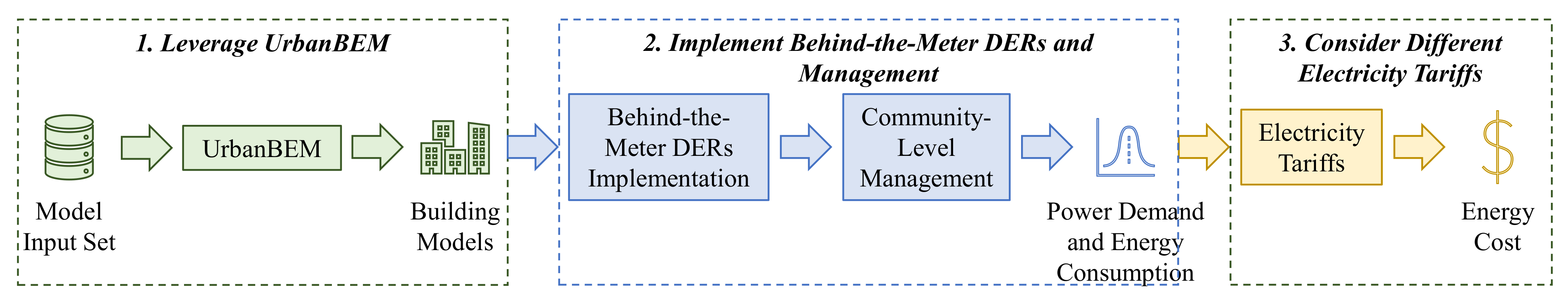
2. Community-Scale Building Energy Modeling Tool

This section introduces the new community-scale building energy modeling tool. Section 2.1 provides a general description of this tool. Then, Section 2.2, Section 2.3 and Section 2.4 detail the three parts of this tool, respectively.

2.1. General Description

Figure 1 outlines the structure of this community-scale building energy modeling tool. This tool leverages the authors’ previous Urban-scale Building Energy Modeling (UrbanBEM) framework [21] to generate community-scale building energy models. Then, behind-the-meter DERs can be implemented into some building models and community-level management strategies need to be provided. In addition, various electricity tariffs are provided. Based on the simulated power demand and energy consumption, the annual energy cost can be calculated. The following section will provide more details about these three parts.

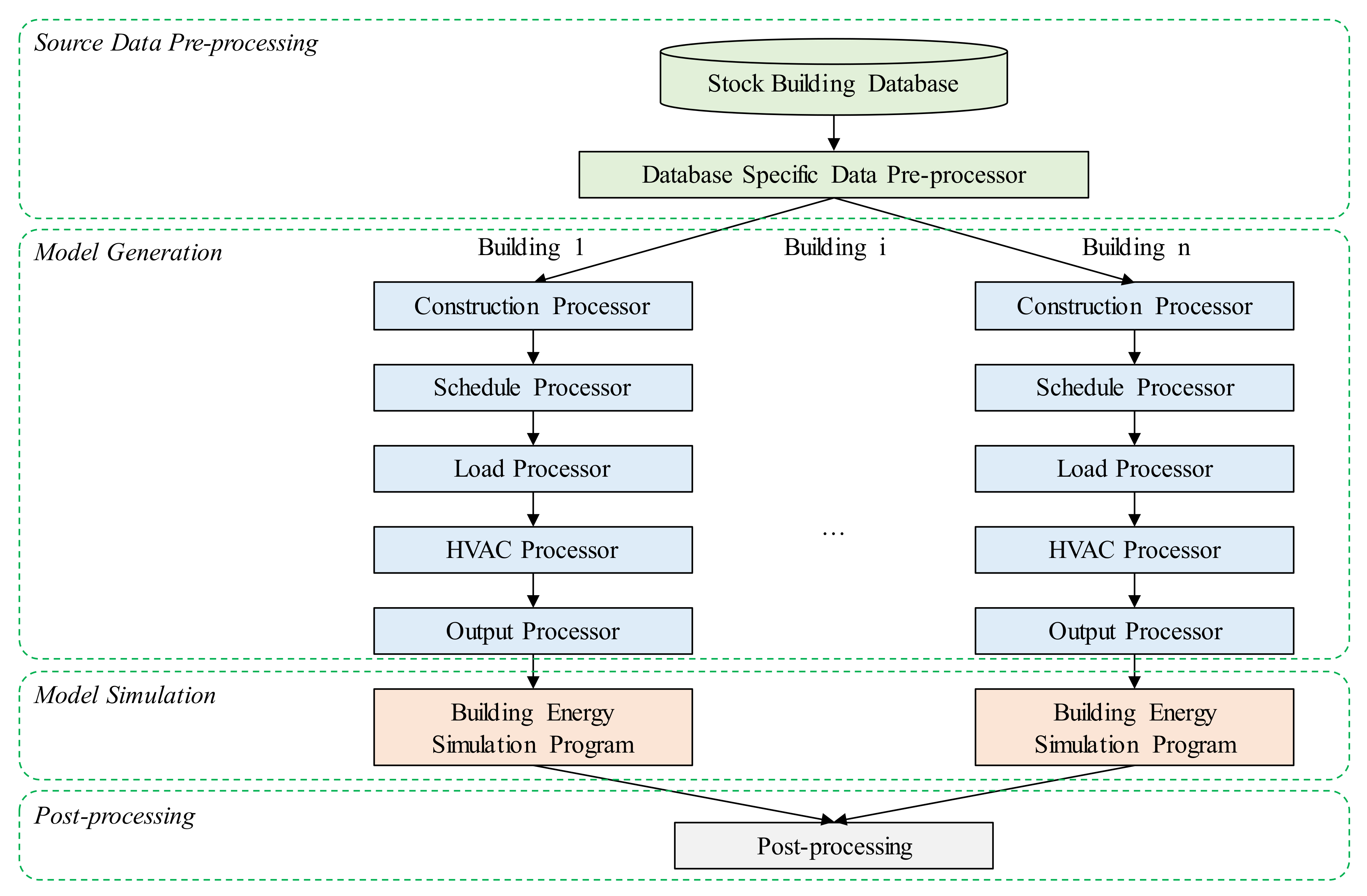
2.2. UrbanBEM

Building energy models in a virtual community are developed by a modularized urban-scale building modeling framework designed for heterogeneous datasets. This framework is developed by Pacific Northwest National Laboratory (PNNL) [21]. Figure 2 visualizes the workflow of this framework.

The framework consists of four steps: (1) source data preprocessing, (2) model generation, (3) model simulation, and (4) postprocessing. In Step 1, the dataset preprocessing module is unique for different datasets. The raw data from the corresponding dataset are translated into information items specified by the standardized model input schema, such as building area type, number of floors, and lighting power density. In Step 2, based on the standardized model inputs, building energy models are developed by using the five processors: construction, schedule; load; heating, ventilation, and air conditioning system (HVAC); and output. This step is conducted in parallel to reduce the computation time. In Step 3, the building energy models are simulated by using EnergyPlus^TM [31], which is a full-scale building energy modeling program. This step is also conducted in parallel. It is noticed that, to develop a building energy model, more data are needed than standardized model inputs. UrbanBEM provides methods to identify other input data from the standardized model inputs. For example, based on the standardized model inputs, hvac_system_type, heating_system_type, and cooling_system_type, UrbanBEM will identify the heating and cooling efficiency from ASHRAE Standard 90.1 [7,32]. In Step 4, after the simulation process, this framework conducts postprocessing for various research purposes, such as evaluating the aggregated power demand on an urban scale. The more detailed description about UrbanBEM is introduced in Lei, et al. [21].

This framework provides three advantages for large-scale building energy research: (1) the building characteristics are described by standardized model inputs schema. Based on different standardized model input elements, this framework generates building energy models with various building characteristics. Compared with the DOE’s Commercial Prototype Building Models [33], this framework is more flexible for developing building models. It reflects special characteristics for individual buildings in the modeling of a diverse portfolio of buildings. (2) This framework is customizable. For example, in this paper, a stochastic schedule generator is implemented in the schedule processor of this framework. This stochastic schedule generator adds random multi-variate Gaussian noise to hourly schedule vectors and uses parametrized covariance matrix to control for noise level and output schedule smoothness. A set of stochastic schedules are generated and then implemented for individual buildings. Buildings usually have different schedules, even if they belong to the same building type. Based on the schedule inputs in the standardized model input set, this framework provides the uncertainties of start and end time for each building. Furthermore, the uncertainties of the occupant behaviors can also be reflected by fluctuating the schedules. This feature can simulate realistic human behaviors, such as moving in and moving out of the buildings. (3) This framework decouples data source format with model generation routines with the standardized model input schema. With data-source-specific preprocessing modules, this framework accepts various data sources with different data formats, which provide a connector to link survey and measured data from different sources to building energy models. Thus, by using the survey and measured data, this framework can predict the real buildings’ energy consumption on a large scale.

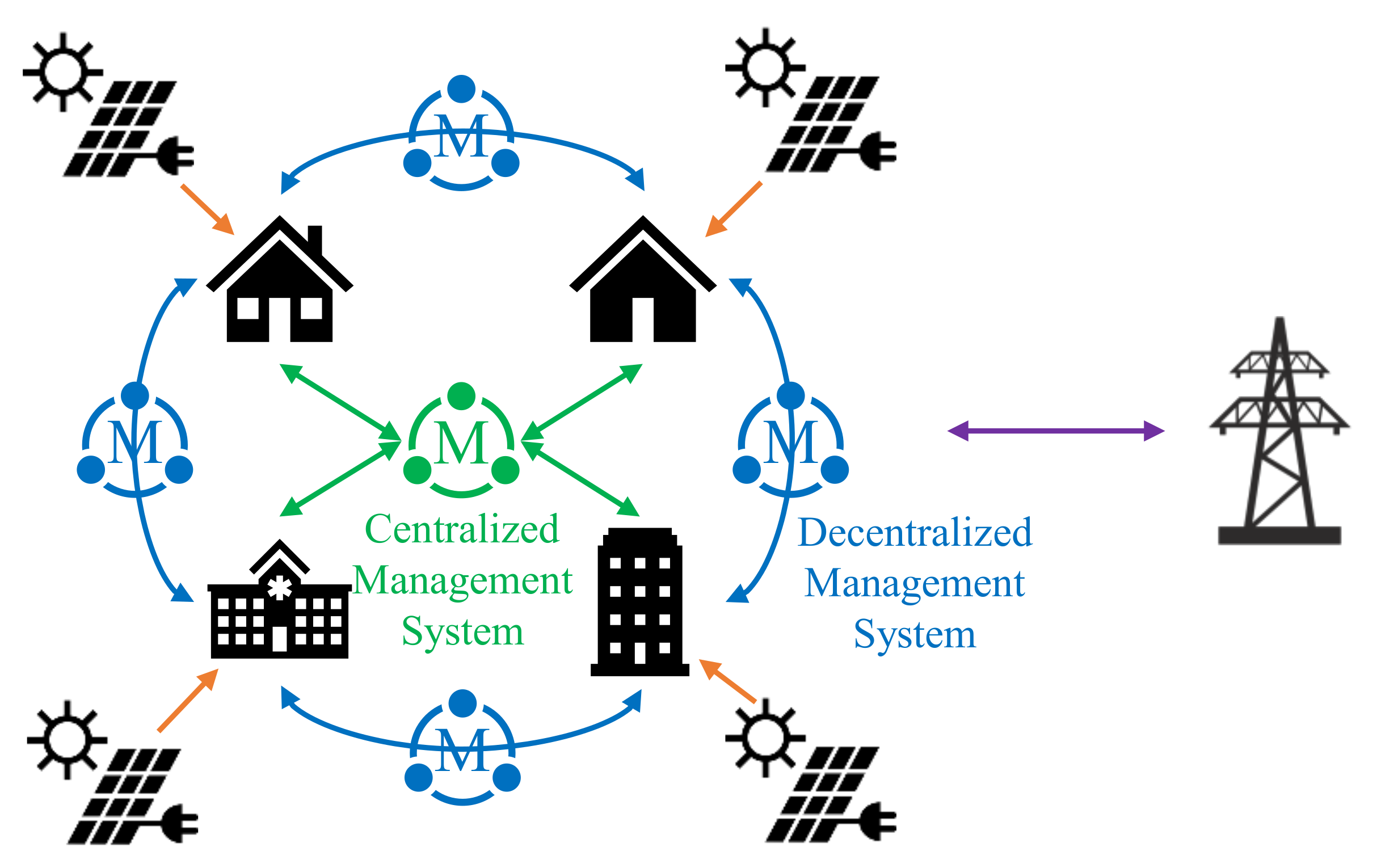
2.3. Behind-the-Meter DERs and Management

The behind-the-meter DERs and community-level power management system are implemented into the building energy models generated by UrbanBEM. The structure is shown in Figure 3. Currently, the new tool can add the rooftop photovoltaics (PV), one type of the behind-the-meter DER, into building energy models. The inputs are: (1) is rooftop PV used for every building; and (2) ratio of PV panel area to roof area.

There are two types of management system: (1) centralized management system and (2) decentralized management system. The centralized management system stores the control strategies in one central control box. The energy-related data are collected from all buildings in the studied community to this central control box. Then, the feedback generated based on the control strategies is sent back to every building. The decentralized management system does not have a central control box. One control box is installed in every building. The data in one building are able to share with other buildings directly and other buildings’ data are also considered for the building control. The final feedback for each building is generated based on the decisions from various control boxes. Using power management systems, the power demand at a community level can be optimized. In addition, this tool allows buildings to share surplus electricity between themselves or sell electricity to the grid. The control logic has been implemented using Python in the community-scale building energy modeling tool. After the building energy models are created and simulated using UrbanBEM, the management system will control electricity consumption and generation.

2.4. Electricity Tariffs

In general, to calculate annual electricity cost, one needs to consider three different types of charges [34,35]: (1) kWh charge, (2) base kW charge, and (3) peak kW charge. kWh charge accounts for the cost of electricity consumption. Base kW charge is applied to the maximum peak demand for each month, regardless of whether it occurs during an off-peak or peak period. Peak kW charge is per peak period and is applied to the maximum peak demand during that peak period in each month. The annual electricity cost can be expressed as follows:

$$\begin{gathered} Annual Electricity Cost = kWh charge + Base kW charge +{\sum }_{i=1}^{n}Peak kW charg{e}_i={\sum }_{i=1}^{365\times 24}\left(kW{h}_i\times \\ kWh unit pric{e}_i\right)+{\sum }_{i=1}^{12}\left(\underset{i}{max}\left(k{W}_j\right)\times base kW unit pric{e}_i\right)+{\sum }_{i=1}^n{\sum }_{m=1}^{12}\left(\underset{m,period i}{max}\left(k{W}_k\right)\times \\ peak kW unit pric{e}_{m,period i}\right), \end{gathered}$$

(1)

where $kW{h}_i$ is the electricity consumption in the ith hour; $kWhunitpric{e}_i$ is the unit price for electricity consumption in the ith hour; $k{W}_j$ is the electricity power in the jth hour, which belongs to the ith month; $basekWunitpric{e}_i$ is the base unit price for electricity power in the ith month; $k{W}_k$ is the electricity power in the kth hour, which belongs to the period i in mth month; $peakkWunitpric{e}_{m,periodi}$ is the peak kW unit price in the period i and mth month, in the peak kW charge; and the total number of the periods is n.

This tool has already implemented three electricity tariffs: (1) ASHRAE Blended [35,36], (2) ASHRAE TOU [34,35], and (3) ConEd Rate III [35,37]. ASHRAE Blended is the standard electricity tariff stated in the ASHRAE 90.1-2022 Work Plan. ASHRAE TOU is the alternative time of use electric rate included in the ASHRAE 90.1-2022 Work Plan. The ConEd Rate III is published under Consolidated Edison New York City, Rate III, General Large Voluntary Time-of-Day and was retrieved from the OpenEI database [37]. The parameters of these three electricity tariffs are listed in

Table 1. Electricity tariffs.

Program	kWh Charge	Base kW Charge	Peak1 kW Charge	Peak2 kW Charge
ASHRAE Blended	$0.11/kWh	-	-	-
ASHRAE TOU	June~September: Peak1: USD 0.11/kWh Non-peak: USD 0.059/kWh October~May: Peak2: $0.095/kWh Non-peak: $0.057/kWh	USD 5.59/kW	June~September: Weekday 1 pm~9 pm: USD 10.99/kW	-
ConEd Rate III	USD 0.012/kWh	June~September: USD 18.36/kW October~May: USD 5.26/kW	June~September: Weekday 8 am~6 pm: USD 28.15/kW October~May: Weekday 8am~9pm: USD 12.43/kW	June~September: Weekday 6 pm~9 pm: USD 19.2/kW

¹ Weekday 1 pm to 9 pm. ² Weekday 6am to 10 am and 5 pm to 9 pm.

.

ASHRAE Blended is a static electricity program and it only considers kWh charge. The kWh unit price is based on published EIA energy data [36]. The unit price is the same for the whole year. Thus, the annual electricity cost is only affected by the annual electricity consumption.

ASHRAE TOU consists of all three charges. The kWh charge has different settings for summer months (June to September) and non-summer months (October to May). The base kW charge has the same setting for all months. It only has one peak kW charge during summer months. Thus, the ASHRAE TOU electricity tariff incentivizes building owners and users to use less electricity during summer, especially during peak periods, since the unit price of kWh charge and peak1 kW charge are both high during these periods.

ConEd Rate III also consists of all three charges. The kWh charge has the same setting for all months. The base kW charge has different settings for summer months (June to September) and non-summer months (October to May). There are two types of peak kW charges. Type 1 (peak1 kW charge) has different settings for summer months and non-summer months, while Type 2 (peak2 kW charge) is only applied for summer months. The variation in the electricity unit price is purely from all-time peak power and peak periods. This pricing program also has the potential to reduce the peak power demand for the power grid.

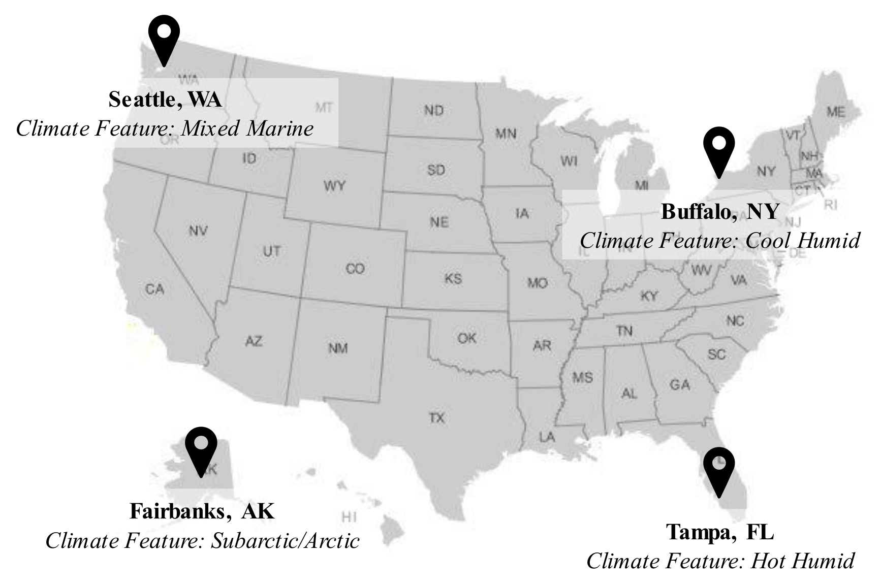
3. Case Description

This section and the next section outline a case study for a virtual community consisting of 22 commercial buildings. The model of these blocks of buildings features four cities for evaluating different climate features and three community scenarios (two traditional community scenarios and one connected community scenario).

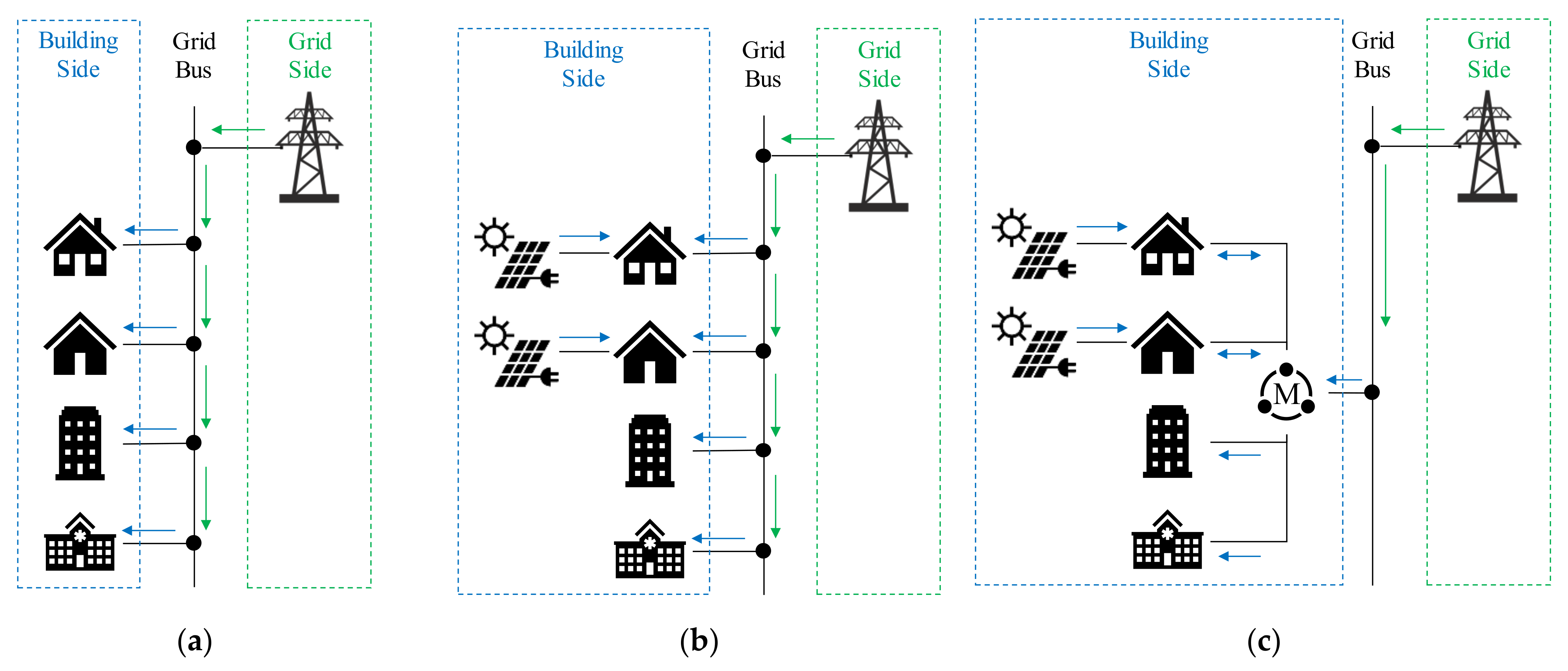
3.1. Scenarios

In this study, we evaluate three community scenarios, which are displayed in Figure 4. All three scenarios in Figure 4 include the two sides of electricity distribution to buildings: (1) grid side and (2) building side. The two sides are connected via the grid bus, which facilitates electricity transmission and distribution. To simplify the study, this paper assumes that the electricity generated by PV panels cannot be sold to the power grid.

Scenario 1, shown in Figure 4a, is a traditional community scenario. All buildings are passive energy users and energy-related actions of these buildings are independent of each other. The power grid generates electricity, and the electricity is supplied to the buildings by the grid bus.

Scenario 2, shown in Figure 4b, is another traditional community scenario. In this scenario, some buildings install PV panels. Thus, these buildings are not only energy users, but also energy generators. The first option for these buildings is to consume the electricity generated by the PV panels. If the electricity generated by the PV panel is lower than the power demand for a building, it will use the electricity supplied by the power grid.

Scenario 3, shown in Figure 4c, is a connected community scenario. Similarly, some buildings install PV panels. If the electricity generated by the PV panel is lower than the power demand for a building, the same strategy as Figure 4b is used; however, if the electricity generated by the PV panel is higher, the surplus electricity will be used for the building without PV panel. A power management system is used to manage the electricity between buildings, and between the buildings and power grid. Usually, there is less electricity surplus in a connected community than a traditional community with PV panels (Scenario 2).

3.2. Building Energy Models

There are many building energy data sources [38], such as U.S. EIA’s Commercial Buildings Energy Consumption Survey (CBECS) [39], Northwest Energy Efficiency Alliance’s (NEEA’s) Commercial Building Stock Assessment (CBSA) [40], and California Energy Commission’s (CEC’s) Commercial End-Use Survey (CEUS) [41]. In this study, the 2012 CBECS [42] is used as the data source, which provides information about the buildings’ characteristics and operations. After data cleansing, we created building energy models for 3515 building samples in the 2012 CBECS. Then, we conducted validation for these building energy models. The Pearson correlation coefficient between the models and the empirical data from the 2012 CBECS is 0.87, and the electricity use predicted by the simulations achieves a coefficient of determinization (R²) of 0.76. The more detailed description about the model development and validation is introduced in Lei, et al. [21].

Among these building models, we selected 22 buildings to form a virtual community for the analyses in this paper and stored them in the stock building database introduced in Section 2.2. Two rules for selecting buildings are as follows: (1) building samples shall contain a variety of building types with different building characteristics and operation styles, and (2) tall buildings (i.e., more than three floors) are not considered.

Table 2. Key parameters of buildings in a virtual community.

Building ID	Building Type	Total Floor Area (m2)	Window-to-Wall Ratio	Number of Floors	Wall Type	Roof Type	People Density (#/100 m2)	Lighting Power Density (W/m2)	Plug Load Density (W/m2)	HVAC System Type
1	Retail	1045	0.500	2	Mass	IEAD	3.55	35.52	3.72	PSZ-AC
2	Office	952	0.050	2	Mass	Attic and Other	1.94	19.38	9.24	VAV Reheat
3	Office	1022	0.180	1	Mass	Attic and Other	1.08	10.76	9.13	PSZ-AC
4	Office	1394	0.180	1	Mass	Attic and Other	1.94	19.38	9.84	PSZ-AC
5	Office	242	0.180	1	Mass	Attic and Other	1.94	19.38	10.15	PSZ-AC
6	Office	102	0.180	1	Wood Framed	Attic and Other	1.94	19.38	9.94	PSZ-AC
7	Office	344	0.050	1	Wood Framed	IEAD	1.94	19.38	9.67	PSZ-AC
8	Office	4181	0.180	3	Mass	IEAD	1.94	19.38	10.00	PSZ-AC
9	Dining: cafeteria/fast food	836	0.180	1	Wood Framed	IEAD	1.40	13.99	10.10	PSZ-AC
10	Dining: Bar lounge/leisure	790	0.500	3	Mass	Attic and Other	2.69	26.91	10.43	PSZ-AC
11	Hotel/Motel	1115	0.050	2	Mass	IEAD	2.58	25.83	3.26	PSZ-AC
12	Hotel/Motel	1301	0.050	2	Mass	Attic and Other	2.58	25.83	3.61	PSZ-AC
13	School/university	697	0.005	1	Mass	Metal Building	2.15	21.53	2.13	PSZ-AC
14	School/university	1115	0.500	1	Mass	Attic and Other	2.15	21.53	4.64	PSZ-AC
15	School/university	24,155	0.180	2	Mass	IEAD	2.15	21.53	2.41	VAV Reheat
16	Religious building	706	0.050	2	Mass	Attic and Other	2.69	26.91	2.72	PSZ-AC
17	Library	186	0.500	1	Mass	IEAD	2.05	20.45	14.41	PSZ-AC
18	Police station	399	0.050	1	Metal Building	Metal Building	1.08	10.76	12.49	PSZ-AC
19	Healthcare clinic	367	0.180	1	Mass	IEAD	1.83	18.30	8.43	PSZ-AC
20	Hospital	1022	0.380	1	Mass	Attic and Other	2.48	24.76	12.47	PSZ-AC
21	Dormitory	1394	0.050	2	Mass	Attic and Other	1.94	19.38	3.69	PSZ-AC
22	Exercise center	604	0.500	2	Mass	Attic and Other	1.08	10.76	6.01	PSZ-AC

shows the key parameters of these 22 buildings.

This virtual community consists of different types of buildings, such as retail and office buildings. Buildings within each building type also have various characteristics. For example, buildings #2 and #6 are both office buildings. Building #2 is 1022 m² and its window-to-wall ratio is only 5%, while building #6 is much smaller and its window-to-wall ratio is larger. Furthermore, the wall and roof types, internal loads, and HVAC system types are different in these two buildings. Buildings with different characteristics will potentially benefit from sharing energy within a connected community due to different preferences and energy requirements.

To compare the performance of traditional and connected communities, three scenarios were designed, shown in Figure 4. Scenarios 1 and 2 are traditional communities, which are shown in Figure 4a,b, respectively; Scenario 3 is a connected community schema, which is shown in Figure 4c.

Table 3. PV panels installed in the three scenarios.

Building ID	Building Type	Scenario 1 (Electricity only Supplied by the Grid)	Scenario 2 (PV Panels Installed in Some Buildings)	Scenario 3 (Connected Community)
1	Retail	No PV	No PV	No PV
2	Office	No PV	PV (100% roof area)	PV (100% roof area)
3	Office	No PV	PV (100% roof area)	PV (100% roof area)
4	Office	No PV	PV (100% roof area)	PV (100% roof area)
5	Office	No PV	PV (100% roof area)	PV (100% roof area)
6	Office	No PV	PV (100% roof area)	PV (100% roof area)
7	Office	No PV	PV (100% roof area)	PV (100% roof area)
8	Office	No PV	PV (100% roof area)	PV (100% roof area)
9	Dining: cafeteria/fast food	No PV	No PV	No PV
10	Dining: bar lounge/leisure	No PV	No PV	No PV
11	Hotel/Motel	No PV	No PV	No PV
12	Hotel/Motel	No PV	No PV	No PV
13	School/university	No PV	PV (100% roof area)	PV (100% roof area)
14	School/university	No PV	PV (100% roof area)	PV (100% roof area)
15	School/university	No PV	PV (100% roof area)	PV (100% roof area)
16	Religious building	No PV	No PV	No PV
17	Library	No PV	No PV	No PV
18	Police station	No PV	No PV	No PV
19	Healthcare clinic	No PV	No PV	No PV
20	Hospital	No PV	No PV	No PV
21	Dormitory	No PV	No PV	No PV
22	Exercise center	No PV	No PV	No PV

shows whether PV panels are installed in each scenario. The EnergyPlus^TM object, PHOTOVOLTAICPERFORMANCE:SIMPLE, is used to implement PV into buildings. The cell efficiency is 0.12 for all cases. To simplify the case, we do not consider different ratios of PV panel area to roof area. It becomes an either/or question: no PV or PV on the whole roof area. In Scenario 1, there is no PV panel for all buildings in this community. In Scenarios 2 and 3, we assume that all office and school/university buildings install PV panels.

Furthermore, this study also considers the impact of climate to the performance of the connected community. Four cities with different climate features were selected (Figure 5). Tampa, FL, is in the southeastern U.S., which is hot and humid; Buffalo, NY, is in northeastern U.S., which is cool and humid; Seattle, WA, is in northwestern U.S., which is mixed marine climate; Fairbanks, AK, is extremely far north, has a subarctic/arctic climate, and is extremely cold.

To reflect the uncertainties of occupant behaviors in different buildings, we provide the specific schedules for each building. This paper randomizes the start and end time and fluctuates the fraction of each hour but does not randomize the lunchtime. Figure 6 displays the occupancy schedule examples for all 22 studied buildings. Figure 6a shows an example for a workday and Figure 6b is an example for a weekend day. An occupancy schedule here is the fraction of actual occupant density over default occupancy density for every hour. The value for each hour is between 0 and 1. The darker red color means higher fraction and vice versa. In general, different building types have various occupancy preferences. For example, office buildings usually have more people during the workday’s daytime, while hotels/motels have more people at night. Office buildings include lunchtime, which is from 12:00pm to 1:00pm. Furthermore, at a specific time, some people in a building leave the building, while some others enter the building. Thus, the schedules have variant hourly occupancy fractions, reflected by the shades of red color in Figure 6.

By using the framework introduced in Section 2.2, the energy-related data of different end uses for the selected 22 buildings is calculated with respect to the four cities. Figure 7 shows the annual end-use energy consumptions for each building model in these four studied cities. The energy consumption per area is used, known as energy use intensity (EUI).

The distributions of annual end-use EUIs in different buildings in different locations vary. In general, all buildings in Tampa, FL, consume more energy for cooling than heating, while all buildings in other cities consume more for heating. The electricity consumed for a fan is similar, and the energy for lighting and equipment is the same in all the four studied cities. Buildings #10, #11, #12, #20, and #21 have higher EUIs compared with the others because they have longer operation hours. Furthermore, differences in energy efficiency of lighting fixtures and equipment, envelopes, and system types also contribute to the diversity in EUIs between buildings.

4. Case Result

This section analyzes the simulation results for the three scenarios. Section 4.1 introduces the power demand in these three scenarios, using five summer days as an example; Section 4.2 shows the community-level annual electricity consumption in all four studied cities; Section 4.3 summarizes the community-level annual cost for electricity consumption by considering all three electricity tariffs shown in Table 1.

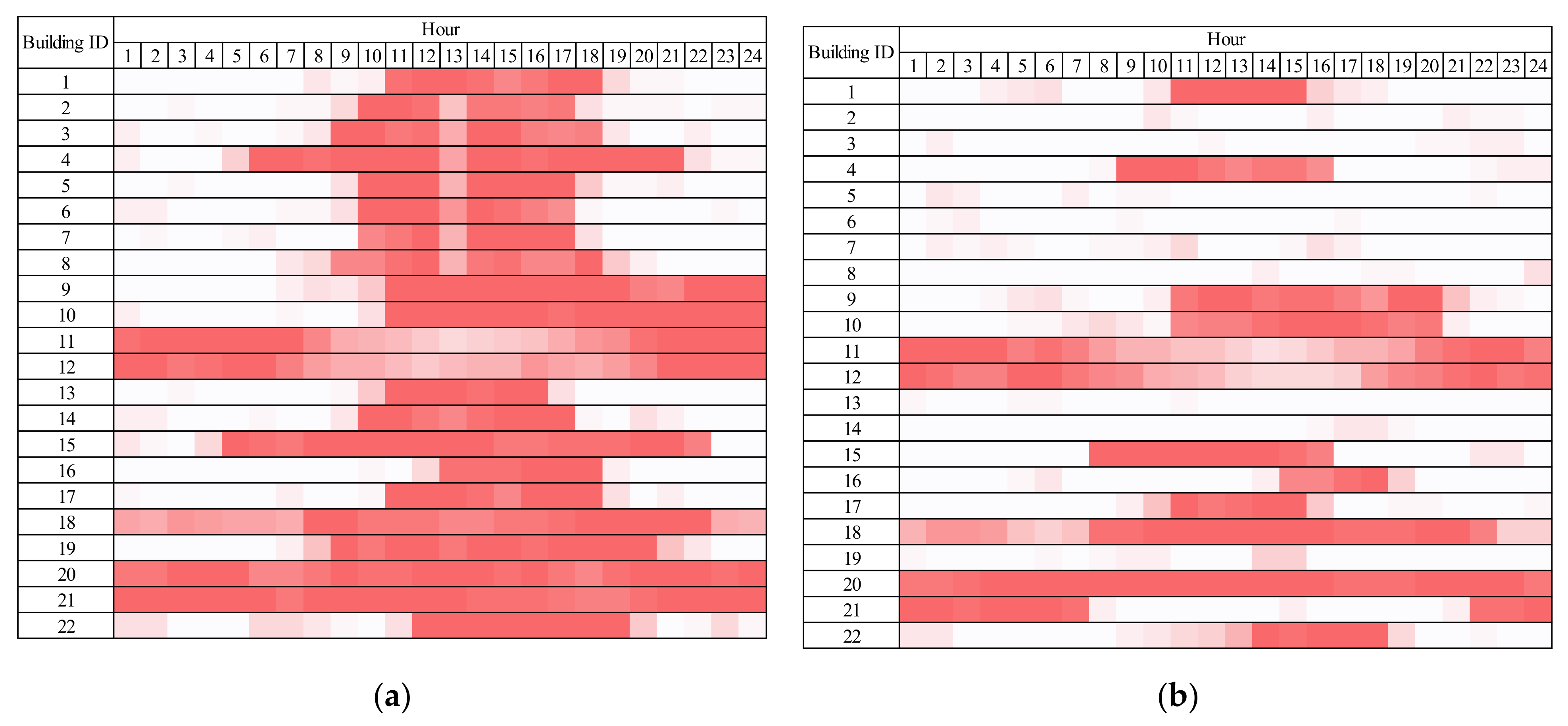
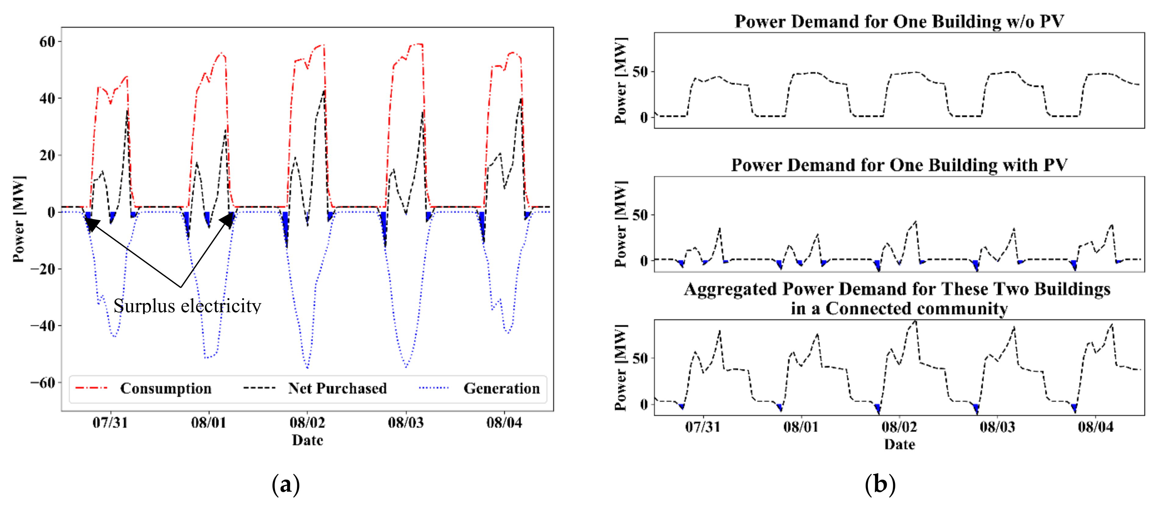
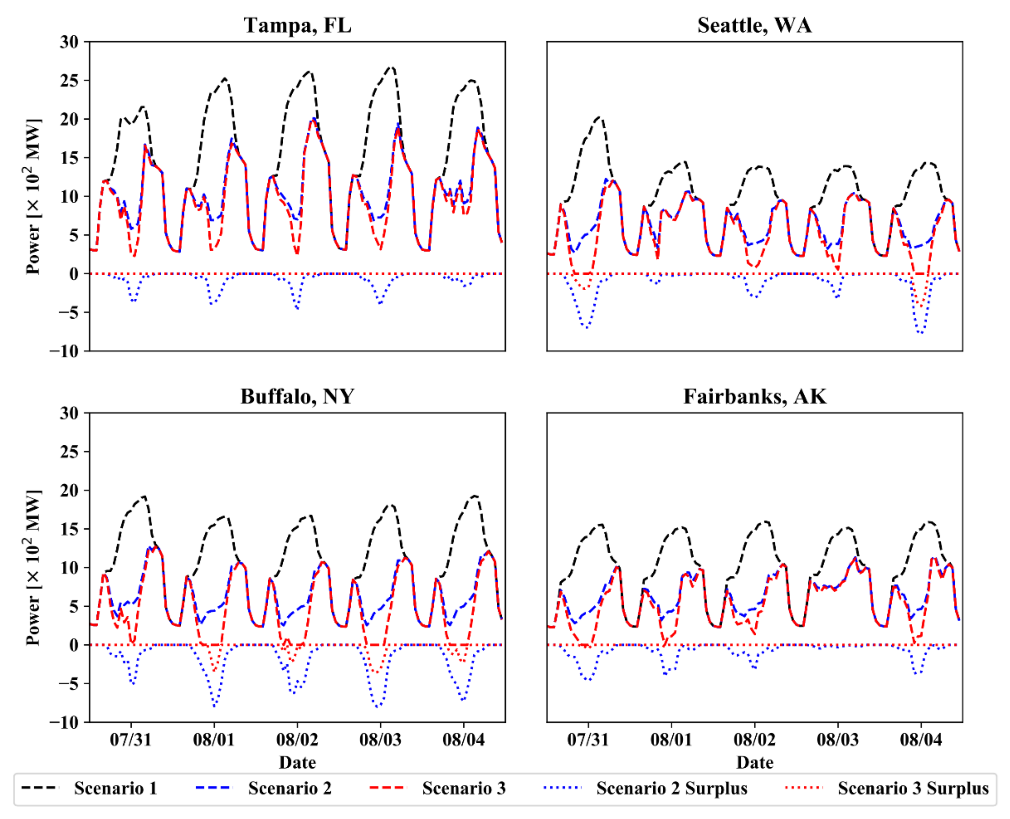
4.1. Power Demand

The power demand is a time-series variable, and we use hourly sampled power demand from the simulation results in this study. Figure 8 visualizes electricity sharing in a connected community. Figure 8a shows the electricity generation and consumption in one building with PV. The first option of electricity sources for this building is the electricity generated by PV panel. However, the electricity generated by the PV panel cannot always meet the power demand of the building. Thus, during such periods, the building consumes electricity provided by the power grid. Furthermore, during certain hours, electricity generated by PV surpasses the power demand of the building on which the PV is installed. In Scenario 2, all surplus electricity is wasted. However, in a connected community (Scenario 3), buildings with PV panel share the surplus electricity with buildings without PV (Figure 8b). Thus, the total surplus electricity in the connected community (Scenario 3) is less than that of the nonconnected community (Scenario 2).

The aggregated power demand is also a time-series variable representing the sum of the power demands for all buildings. To demonstrate the aggregated power demand in the three scenarios introduced in Figure 4, five summer days (31 July to 4 August) are selected. Figure 9 shows the aggregated power demand of the communities in the four studied cities during these five days. The dashed lines represent the aggregated power demand of the community in the three scenarios. The dotted lines represent the total surplus electricity power in Scenarios 2 and 3.

During the five days shown in Figure 9, the community for Scenario 1 in Tampa, FL, has the highest aggregated power demand for most of the daytime among the four studied cities. The peak aggregated power demand in these five days is approximately 2500 MW in Tampa, FL. The power demand is approximately 2000 MW in Seattle, WA, and Buffalo, NY, while 1500 MW in Fairbanks, AK. By installing PV panels in all office and school/university buildings, the aggregated peak power demand in these five days is reduced by approximately 500 MW, which is 25% to 33% of the peak value in these cases. However, in Scenario 2, some electricity generated by the PV panels is surplus in all four cases. More than 500 MW power is sometimes surplus in all the four locations. By sharing electricity between buildings in Scenario 3, the surplus electricity is reduced. The cases in Tampa, FL, and Fairbanks, AK, do not have any surplus electricity in these five days.

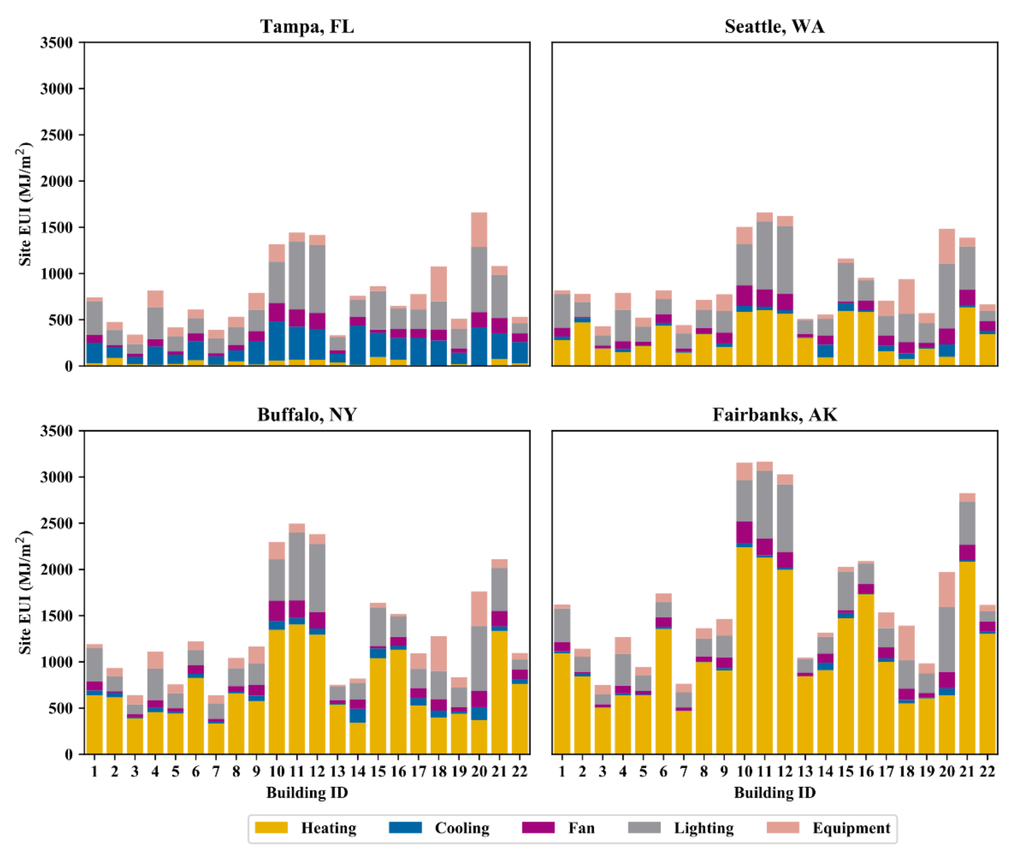
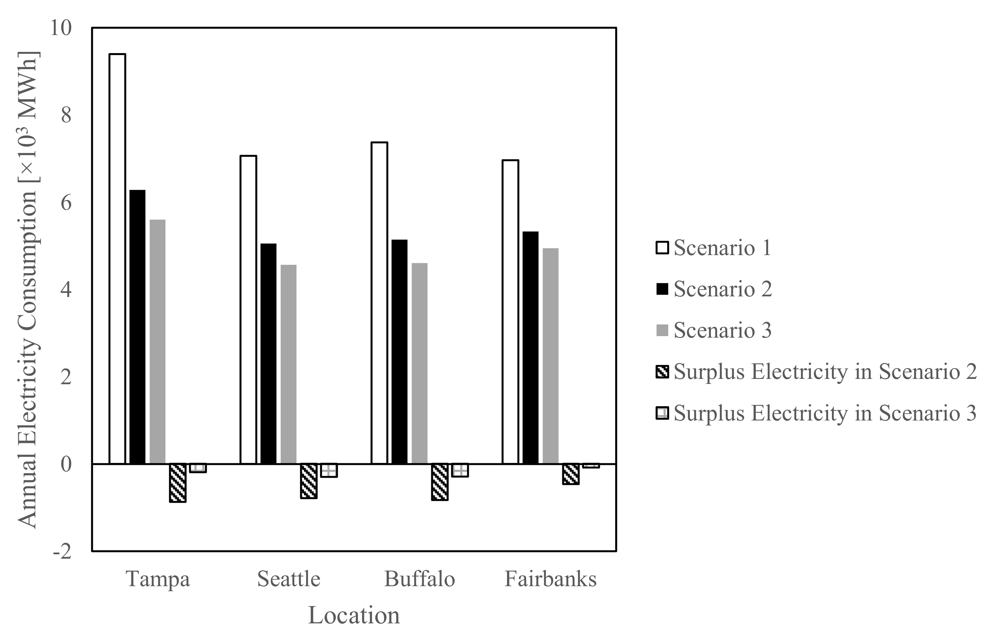
4.2. Annual Electricity Consumption

The aggregated annual electricity consumption shows the total electricity consumption in the studied community for a whole year. Figure 10 displays the aggregated annual electricity consumption and the result quantifies the electricity saving in the connected community. The figure provides the aggregated annual electricity consumption for three scenarios in the four studied cities and the aggregated annual surplus electricity for Scenarios 2 and 3.

In Scenario 1, the aggregated annual electricity consumption of the virtual community is approximately 9500 MWh in Tampa, FL, versus approximately 7500 MWh in the rest of the three cities. In Scenario 2, by utilizing electricity generated by the PV panels, the aggregated annual electricity consumption is reduced by 1600 MWh to 3100 MWh, which is 25% to 33% of the total electricity consumption. However, 460 MWh to 870 MWh of electricity generated by the PV panels is surplus in all four cases, since the generated electricity exceeds the demand in some buildings during some periods. In Scenario 3, due to sharing electricity between buildings, some surplus electricity for some buildings is used for some other buildings that need electricity. Thus, the aggregated annual electricity consumption of the virtual community is further reduced by 400 MWh to 700 MWh, which is 5.5% to 7.3% of the total electricity consumption in Scenario 1. The annual total surplus electricity in all four cases is decreased, which is lower than 300 MWh. Especially in Fairbanks, the annual total surplus electricity is only 80 MWh, which is only 1% of the aggregated annual electricity consumption in Scenario 1.

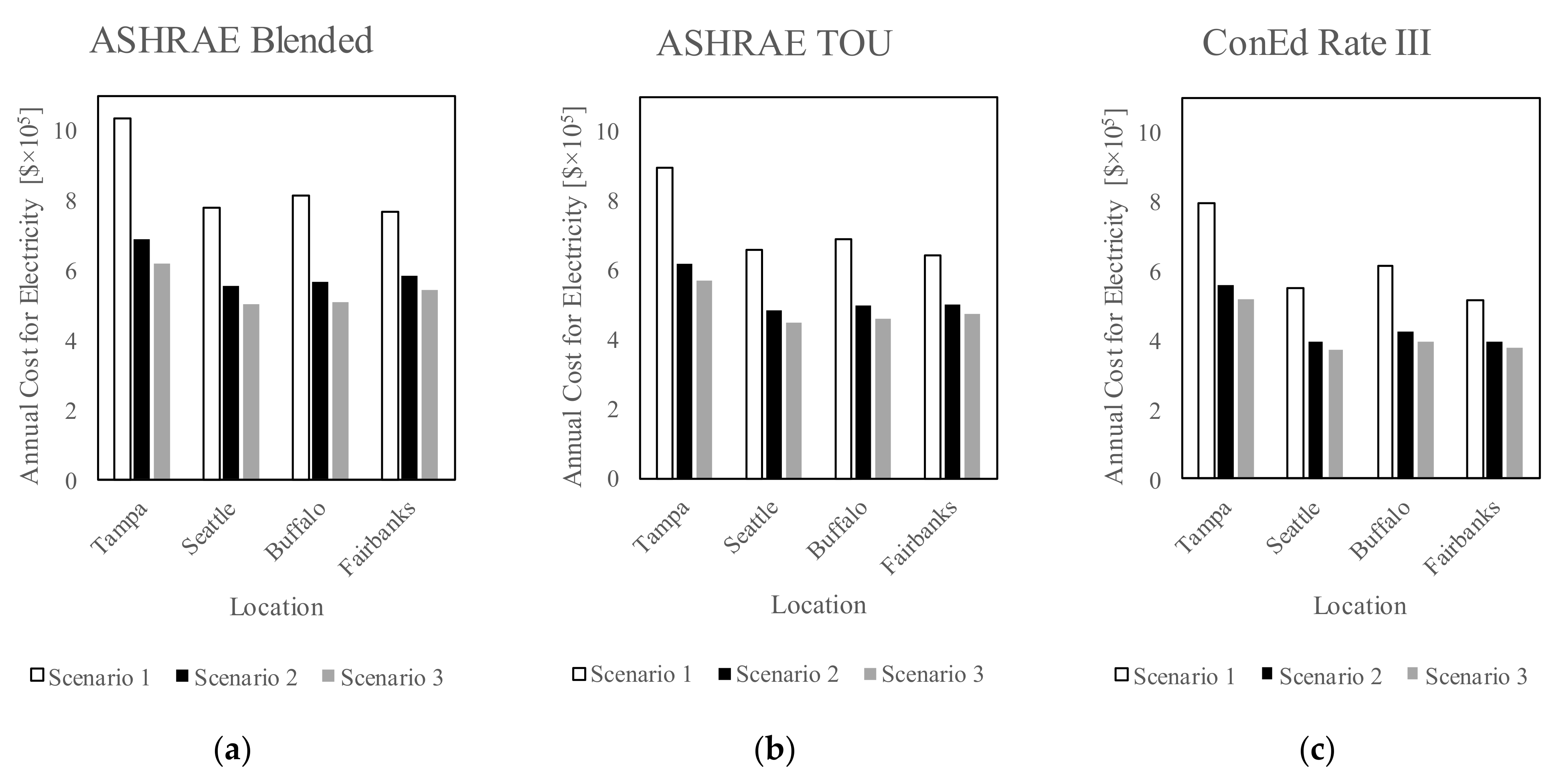
4.3. Annual Electricity Cost

The aggregated annual electricity cost shows the total electricity cost in the studied community for a whole year. By using the three electricity tariffs introduced in Section 3, the aggregated annual electricity costs are calculated. The results are shown in Figure 11. The figure provides the aggregated annual electricity costs for the studied communities in the three scenarios located in the four studied cities.

The aggregated annual electricity cost by using the ASHRAE Blended pricing program is higher than the other two pricing programs in all three scenarios and four cities. The ConEd Rate III results in the lowest cost among the three pricing programs. Due to its high aggregated annual electricity consumption, the community in Tampa, FL, has the highest aggregated annual electricity cost compared with the other three locations in all three pricing programs and three scenarios. By implementing the PV panels for some buildings (from Scenario 1 to Scenario 2), the annual cost can be reduced by USD 100,000 to USD 300,000 for different cases, which is approximately 20% to 30% reduction in the total cost. Furthermore, by connecting buildings together (from Scenario 2 to Scenario 3), the annual cost can be further reduced by USD 20,000 to USD 75,000 for different cases, which is approximately 5% to 11% of total cost.

5. Discussion

This paper develops a new community-scale building energy modeling tool and presents a case study comparing power demand, annual electricity consumption, and annual electricity cost in a community. Different buildings have various geometries, envelopes, internal loads, and HVAC systems. In addition, different building types, such as office, retail, and school/university buildings have different operation preferences. Some building types, such as office buildings, are usually operated during daytime. However, in building types such as hotel/motel buildings, guests typically go outside during the daytime and go to sleep at night. Thus, these building types tend to have more people at night. Some other building types, such as hospitals, are operated 24/7. These buildings are occupied all the time. Thus, a connected community which shares energy between different building types is a future research direction. A community-scale building energy modeling tool is necessary to conduct such research.

The new community-scale building energy modeling tool introduced in this paper considers the various characteristics and stochastic operation schedules for buildings. PV panels and energy sharing strategies are also implemented. In addition, three electricity tariffs are considered. However, this case is simpler than the real cases. For example, we do not consider the different strategies to install the PV panels. We do not consider the batteries and selling electricity to the power grid. We do not consider optimized control using advanced building technologies as well. All of them will make connected community study far more complex. In the future, there are three research directions for the tool development and its applications:

• In the case study, the PV panels are installed on the roofs of all office and school/university buildings. If the PV panels are installed on other buildings’ roofs or the sizes of the PV panels are changed, the electricity consumption and cost will be different. The total size of the PV panels impacts the results of electricity consumption and cost. Assuming the parameters of PV panels, such as tilt angle and system losses, are constant and that there is no shade, the electricity generated by the PV panels is linear with respect to the total size of the PV panels. Thus, the suitable size of the PV panels needs to be studied in future work. If the roof area is not sufficient, some other areas, such as parking lots, are also considered.
• Installing batteries for PV panels and selling electricity to the power grid are also strategies to reduce electricity consumption and cost. We plan to implement the batteries into the tool. In addition, in this case study, we do not consider selling electricity to the power grid. In the future, it is also a possible research direction. Based on our current review, there are three potential problems for this research, which we will consider: (1) a battery is expensive. Fu, et al. [43] documents research on the cost of standalone energy storage systems. The cost of battery is USD 209/kWh, which does not include the cost for the installation and maintenance. The initial and maintenance costs are high and the cost effectiveness needs to be studied when this method is considered. (2) It is difficult to estimate the suitable capacity of the batteries. If batteries are selected to store the surplus electricity for buildings with PV panels, it is necessary to estimate the amount of the surplus electricity and then decide a suitable capacity of batteries. (3) The management becomes much more complex if end users can sell electricity to the power grid. Due to the bi-direction electricity supply mechanism, the power grid side is more difficult to estimate the power demand of end users. In our case, due to the different features for buildings, there are many chances to share energy between buildings. Thus, the power grid side can estimate the power demand on the community level and then design the mechanism to supply the electricity from community level to building level, which is easier.
• We will implement some other technologies into this tool. Currently, we only implement PV panels. There are lots of other technologies. For example, U.S. Department of Energy (DOE) has recently promoted grid-interactive efficient buildings [44]. Many advanced building technologies include smart HVAC systems, connected lighting, dynamic windows, occupancy sensing, thermal mass, and distributed generation and battery storage [9,45,46,47,48]. All these technologies can optimize the power demand on a large scale. Furthermore, besides buildings, vehicles, particularly electric vehicles, are one of the end uses of electricity [49] meriting future research.

6. Conclusions

This paper developed a new community-scale building energy modeling tool. Using this tool, a case for a community was studied under three scenarios: (1) electricity only supplied by the grid, (2) PV panels installed on and available to some but not all the buildings, and (3) an electricity connected community. In addition, this case study considered the impacts of location and electricity tariffs on community power demand, annual electricity consumption, and annual electricity cost. The results show that, after some buildings installed PV panels (from Scenario 1 to Scenario 2), the aggregated annual electricity consumption is reduced by 25% to 33% of the total electricity consumption. By sharing the electricity between buildings (from Scenario 2 to Scenario 3), the aggregated annual electricity consumption is further reduced by 5.5% to 7.3% of the total electricity consumption in Scenario 1. Furthermore, due to the reduction in the aggregated annual electricity consumption and peak power load, the annual electricity cost is reduced. From Scenario 1 to Scenario 2, the cost can be reduced by approximately 20% to 30%; from Scenario 2 to Scenario 3, the cost can continue being reduced by approximately 5% to 11%. We will implement new features for this tool and conduct more application studies.

References

- EIA. Annual Energy Outlook 2020: With Projections to 2050; Government Printing Office: Washington, DC, USA, 2020.
- Glazer, J. Development of Maximum Technically Achievable Energy Targets for Commercial Buildings. ASHRAE Trans. 2017, 123, 32. [Google Scholar]
- Halverson, M.A.; Hart, R.; Athalye, R.A.; Rosenberg, M.I.; Richman, E.E.; Winiarski, D.W. Ansi/Ashrae/Ies Standard 90.1-2013 Preliminary Determination: Qualitative Analysis; Pacific Northwest National Lab. (PNNL): Richland, WA, USA, 2014.
- Halverson, M.A.; Rosenberg, M.I.; Hart, P.R.; Richman, E.E.; Athalye, R.A.; Winiarski, D.W. Ansi/Ashrae/Ies Standard 90.1-2013 Determination of Energy Savings: Qualitative Analysis; Pacific Northwest National Lab. (PNNL): Richland, WA, USA, 2014.
- Rosenberg, M.; Hart, R.; Athalye, R.; Zhang, J.; Cohan, D. Potential Energy Cost Savings from Increased Commercial Energy Code Compliance. In Proceedings of the ACEEE Summer Study on Energy Efficiency in Building, Pacific Grove, CA, USA, 21–26 August 2016. [Google Scholar]
- Zhang, J.; Xie, Y.; Athalye, R.A.; Zhuge, J.W.; Rosenberg, M.I.; Hart, P.R.; Liu, B. Energy and Energy Cost Savings Analysis of the 2015 IECC for Commercial Buildings; Pacific Northwest National Lab. (PNNL): Richland, WA, USA, 2015.
- Standard 90.1-2013; Energy Standard for Buildings Except Low-Rise Residential Buildings. ASHRAE: Washington, DC, USA, 2013.
- Wang, K.; Yin, R.; Yao, L.; Yao, J.; Yong, T.; Deforest, N. A two-layer framework for quantifying demand response flexibility at bulk supply points. IEEE Trans. Smart Grid 2016, 9, 3616–3627. [Google Scholar] [CrossRef]
- Neukomm, M.; Nubbe, V.; Fares, R. Grid-interactive Efficient Buildings Technical Report Series: Overview of Research Challenges and Gaps; National Renewable Energy Lab. (NREL): Golden, CO, USA, 2019.
- Hagerman, J. Buildings-to-Grid Technical Opportunities: Introduction and Vision; EERE Publication and Product Library: Washington, DC, USA, 2014.
- DOE. About Buildings-to-Grid Integration. Available online: https://www.energy.gov/eere/buildings/about-buildings-grid-integration (accessed on 1 September 2022).
- Seyedzadeh, S.; Rahimian, F.P.; Oliver, S.; Rodriguez, S.; Glesk, I.J.A.E. Machine learning modelling for predicting non-domestic buildings energy performance: A model to support deep energy retrofit decision-making. Appl. Energy 2020, 279, 115908. [Google Scholar] [CrossRef]
- Seyedzadeh, S.; Rahimian, F.P.; Rastogi, P.; Glesk, I. Tuning machine learning models for prediction of building energy loads. Sustain. Cities Soc. 2019, 47, 101484. [Google Scholar] [CrossRef]
- Hale, E.; Horsey, H.; Johnson, B.; Muratori, M.; Wilson, E.; Borlaug, B.; Christensen, C.; Farthing, A.; Hettinger, D.; Parker, A. The Demand-Side Grid (dsgrid) Model Documentation; National Renewable Energy Lab. (NREL): Golden, CO, USA, 2018.
- Chen, Y.; Hong, T.; Piette, M.A. Automatic generation and simulation of urban building energy models based on city datasets for city-scale building retrofit analysis. Appl. Energy 2017, 205, 323–335. [Google Scholar] [CrossRef]
- Ingraham, J.A.; New, J.R. Virtual EPB. Build. Technol. Off. Follow. BTO Peer Rev. 2018, 87. [Google Scholar]
- NREL. ComStock Analysis Tool. Available online: https://www.nrel.gov/buildings/comstock.html (accessed on 1 September 2022).
- Polly, B.; Kutscher, C.; Macumber, D.; Schott, M.; Pless, S.; Livingood, B.; Van Geet, O. From zero energy buildings to zero energy districts. In Proceedings of the American Council for an Energy Efficient Economy Summer Study on Energy Efficiency in Buildings, Pacific Grove, CA, USA, 21–26 August 2016; pp. 21–26. [Google Scholar]
- Reinhart, C.; Dogan, T.; Jakubiec, J.A.; Rakha, T.; Sang, A. Umi-an urban simulation environment for building energy use, daylighting and walkability. In Proceedings of the 13th Conference of International Building Performance Simulation Association, Chambery, France, 26–28 August 2013. [Google Scholar]
- Wilson, E.J.; Christensen, C.B.; Horowitz, S.G.; Robertson, J.J.; Maguire, J.B. Energy Efficiency Potential in the US Single-Family Housing Stock; National Renewable Energy Lab. (NREL): Golden, CO, USA, 2017.
- Lei, X.; Ye, Y.; Lerond, J.; Zhang, J. A Modularized Urban Scale Building Energy Modeling Framework Designed with An Open Mind. In Proceedings of the 2021 ASHRAE Winter Conference, Chicago, IL, USA, 9–11 February 2021. [Google Scholar]
- Wang, J.; El Kontar, R.; Jin, X.; King, J. Electrifying High-Efficiency Future Communities: Impact on Energy, Emissions, and Grid. Adv. Appl. Energy 2022, 6, 100095. [Google Scholar] [CrossRef]
- El Kontar, R.; Polly, B.; Charan, T.; Fleming, K.; Moore, N.; Long, N.; Goldwasser, D. URBANopt: An Open-Source Software Development Kit for Community and Urban District Energy Modeling; National Renewable Energy Lab. (NREL): Golden, CO, USA, 2020.
- Burleyson, C.D.; Iyer, G.; Hejazi, M.; Kim, S.; Kyle, P.; Rice, J.S.; Smith, A.D.; Taylor, Z.T.; Voisin, N.; Xie, Y. Future western US building electricity consumption in response to climate and population drivers: A comparative study of the impact of model structure. Energy 2020, 208, 118312. [Google Scholar] [CrossRef]
- Abdullahi, D.; Renukappa, S.; Suresh, S.; Oloke, D. Barriers for implementing solar energy initiatives in Nigeria: An empirical study. Smart Sustain. Built Environ. 2021. ahead of print. [Google Scholar] [CrossRef]
- IECC. International Energy Conservation Code 2015. In C406; IECC: Washington, DC, USA, 2015. Available online: https://codes.iccsafe.org/content/IECC2015/chapter-4-re-residential-energy-efficiency (accessed on 1 September 2022).
- Pless, S.; Torcellini, P. Net-Zero Energy Buildings: A Classification System Based on Renewable Energy Supply Options; National Renewable Energy Lab. (NREL): Golden, CO, USA, 2010.
- Olgyay, V.; Coan, S.; Webster, B.; Livingood, W. Connected Communities: A Multi-Building Energy Management Approach; National Renewable Energy Lab. (NREL): Golden, CO, USA, 2020.
- Ye, Y.; Lou, Y.; Zuo, W.; Franconi, E.; Wang, G. How do electricity pricing programs impact the selection of energy efficiency measures?–A case study with US Medium office buildings. Energy Build. 2020, 224, 110267. [Google Scholar]
- Hao, H.; Corbin, C.D.; Kalsi, K.; Pratt, R.G. Transactive control of commercial buildings for demand response. IEEE Trans. Power Syst. 2016, 32, 774–783. [Google Scholar] [CrossRef]
- Crawley, D.B.; Lawrie, L.K.; Pedersen, C.O.; Winkelmann, F.C. Energy plus: Energy simulation program. ASHRAE J. 2000, 42, 49–56. [Google Scholar]
- Roth, A. New OpenStudio-Standards Gem Delivers One Two Punch. Available online: https://www.energy.gov/eere/buildings/articles/new-openstudio-standards-gem-delivers-one-two-punch (accessed on 1 September 2022).
- DOE and PNNL. Commercial Prototype Building Models. Available online: https://www.energycodes.gov/development/commercial/prototype_models (accessed on 1 September 2022).
- Franconi, E.; Lerond, J.; Nambiar, C.; Kim, D.; Rosenberg, M.; Williams, J. Opening the Door to Grid-Interactive Efficient Buildings with Building Energy Codes. In Proceedings of the ACEEE 2020 Summer Study on Energy Efficiency in Buildings, Online, 17–21 August 2020; Paper presented at the PNNL-SA-155693. American Council for an Energy Efficient Economy 2020 Summer Study: Washington, DC, USA. [Google Scholar]
- Lei, X.; Franconi, E.; Ye, Y. Optimizing Price-Informed Operation of a Battery Storage System in an Office Building. In Proceedings of the Building Simulation 2021 Conference, Bruges, Belgium, 1–3 September 2021. [Google Scholar]
- EIA. Annual Energy Outlook 2019: With Projections to 2050; Government Printing Office: Washington, DC, USA, 2019. [Google Scholar]
- OpenEI. View Rate: Consolidated Edison Co-NY Inc. Available online: https://openei.org/apps/USURDB/rate/view/5cd201dc5457a3c62754e9d4#1__Basic_Information (accessed on 1 September 2022).
- Ye, Y.; Zuo, W.; Wang, G. A comprehensive review of energy-related data for US commercial buildings. Energy Build. 2019, 186, 126–137. [Google Scholar] [CrossRef]
- EIA. Commercial Buildings Energy Consumption Survey. Available online: https://www.eia.gov/consumption/commercial/ (accessed on 1 September 2022).
- NEEA. Commercial Building Stock Assessment. Northwest Energy Efficiency Alliance. Available online: https://neea.org/data/commercial-building-stock-assessments (accessed on 1 September 2022).
- CEC. California Commercial End-Use Survey. Available online: https://www.energy.ca.gov/data-reports/surveys/california-commercial-end-use-survey (accessed on 1 September 2022).
- EIA. 2012 CBECS Survey Data. Available online: https://www.eia.gov/consumption/commercial/data/2012/ (accessed on 1 September 2022).
- Fu, R.; Remo, T.W.; Margolis, R.M. 2018 US Utility-Scale Photovoltaics-Plus-Energy Storage System Costs Benchmark; National Renewable Energy Lab. (NREL): Golden, CO, USA, 2018. [Google Scholar]
- DOE. Grid-Interactive Efficient Buildings. Available online: https://www.energy.gov/eere/buildings/grid-interactive-efficient-buildings (accessed on 1 September 2022).
- Goetzler, B.; Guernsey, M.; Kassuga, T.; Young, J.; Savidge, T.; Bouza, A.; Neukomm, M.; Sawyer, K. Grid-Interactive Efficient Buildings Technical Report Series: Heating, Ventilation, and Air Conditioning (HVAC); Water Heating; Appliances; and Refrigeration; National Renewable Energy Lab. (NREL): Golden, CO, USA, 2019.
- Harris, C.; Mumme, S.; LaFrance, M.; Neukomm, M.; Sawyer, K. Grid-Interactive Efficient Buildings Technical Report Series: Windows and Opaque Envelope; National Renewable Energy Lab. (NREL): Golden, CO, USA, 2019.
- Nubbe, V.; Yamada, M.; Walker, B.; Neukomm, M.; Sawyer, K. Grid-Interactive Efficient Buildings Technical Report Series: Lighting and Electronics; National Renewable Energy Lab. (NREL): Golden, CO, USA, 2019.
- Roth, A.; Reyna, J. Grid-Interactive Efficient Buildings Technical Report Series: Whole-Building Controls, Sensors, Modeling, and Analytics; National Renewable Energy Lab. (NREL): Golden, CO, USA, 2019.
- Kempton, W.; Tomić, J. Vehicle-to-grid power fundamentals: Calculating capacity and net revenue. J. Power Sources 2005, 144, 268–279. [Google Scholar] [CrossRef]