Biaxial Testing of Thin Metal Sheets under Non-Proportional Loading Conditions

Abstract

During the manufacturing and service of thin metal sheets, different stress states occur, often caused by non-proportional loading conditions. They can lead to localization of inelastic deformations as well as to damage and failure processes. In the present paper, a series of experiments with newly designed biaxially loaded specimens is presented to analyze the damage and failure behavior of thin ductile metal sheets under non-proportional load paths. Bands of holes with different orientation have been milled in critical regions of the specimens to localize stresses and strains. In compression tests, a special downholder is used to avoid buckling. During the loading processes, strain fields in critical regions of the specimens are monitored by digital image correlation technique. After the experiments, fracture surfaces are investigated by scanning electron microscopy showing different damage and fracture modes depending on the loading history. The experiments clearly demonstrate the efficiency of the thin specimens and the experimental program.

1. Introduction

In lightweight applications, high-quality metals and alloys have to be used to fulfill the requirements of improvement of cost efficiency and reduction of energy consumption as well as demands on increases in service lifetime and safety. However, during the manufacturing or service of thin structures, stress-state- and loading-history-dependent damage and fracture processes happen frequently, often leading to the end of lifetime. Hence, in order to avoid the undesired failure events, the optimization of material properties and forming operations is required, which must be based on the detailed knowledge of the behavior of the new materials on the micro- and the macro-scale. Therefore, sophisticated experimental techniques must be able to cover a wide range of loading histories and expected stress states.

In particular, various tests with uniaxially loaded specimens have been used to obtain the first information on the behavior of metals. Experiments with un-notched and differently notched specimens have been proposed by [1,2,3,4,5,6,7,8] or central hole tension specimens by [9,10] to detect inelastic deformation behavior as well as to investigate damage and fracture processes. To study the effect of nearly zero-stress triaxialities caused by shear loading processes, new geometries of uniaxially loaded specimens have been presented by [2,5,6,7,9,11,12]. However, the experiments with the uniaxially loaded specimens only cover a small range of stress states and, thus, new tests with biaxially loaded cruciform specimens have been developed by [13,14,15,16,17,18,19,20,21,22,23,24,25,26] to examine anisotropic plastic behavior or to study limit strains at fracture in metal sheets. These tests use specimens taken from metal sheets with moderate thicknesses between 3 mm and 5 mm, and notches in thickness direction have been milled to localize inelastic deformations as well as damage and failure processes in these critical regions. This philosophy cannot be taken into account in thin sheets with only 1 mm thickness, as the introduction of notches in the thickness direction or regions with reduced thickness for thin sheets (1.5 mm and thinner) is only possible precisely and is only reproducible with a great effort and the associated high costs. Furthermore, when processing in the thickness direction, the surface areas of the material are removed, and therefore no representative part of the material is examined, which is important to consider, especially for thinner sheets. Consequently, following the ideas of [27], localization of damage can here be caused by special geometries with additional holes in critical regions. These geometries are also used in the present investigation.

Usually, many biaxial experiments are driven under proportional load paths. But in many manufacturing processes and the service of structures, loading is non-proportional. In this context, experimental studies with notched cruciform specimens tested under non-proportional loading conditions have been presented by [28,29] to investigate the fracture behavior of aluminum alloys. They showed that their tests with non-proportional paths with tension–tension loading lead to differences in formation of cracks and the final fracture load compared to tests under proportional loading conditions. In addition, [30] carried out experiments with round notched steel specimens with stress triaxiality step-jumps, and revealed different fracture loci under non-proportional loading conditions compared to proportional paths. Further results of tension–torsion tests with hollow cylindrical steel specimens have been presented by [31]. The non-proportional loading paths are caused by changing the ratio of tension and torsion during the experiments. Alternative tension-torsion as well as compression–torsion tests with notched specimens have been performed by [32] with non-proportional loading paths. They reported that the loading histories affect damage accumulation and the point of onset of fracture. Using biaxially loaded specimens, a new experimental program has been proposed by [33,34] considering various non-proportional load paths or pre-loading histories. These investigations elucidated that the loading histories can remarkably affect the damage and fracture mechanisms.

In the present paper, the failure behavior of thin sheets of the aluminum alloy AA6016-T4 is studied in detail. New specimens for biaxial loading are cut from 1 mm thin sheets and are tested under various non-proportional loading conditions. A downholder is used to avoid the buckling of the thin specimens during compressive loadings. Strain fields in the critical regions of the specimens are monitored by digital image correlation. Based on these data, forming limit diagrams are developed. For different load paths, fracture processes are elucidated by scanning electron microscopy. The experimental results demonstrate the efficiency of the new specimens and of the sophisticated experimental program.

2. Material and Methods

The specimens are cut from 1 mm thick sheets of aluminum alloy AA6016-T4, and the chemical composition is shown in

Table 1. Chemical composition based on an analysis by optical emission spectrometer of the aluminum alloy AA6016-T4, 1 mm (% weight).

Si	Fe	Cu	Mn	Mg	Cr	Zn	Ti	Al
1.200	0.238	0.079	0.138	0.384	0.019	0.014	0.020	to balance

.

The systematic analysis of the stress-state-dependent damage and failure behavior of the investigated aluminum alloy is based on experiments with carefully designed biaxially loaded specimens [21,27]. Details of the geometries are shown in Figure 1. In particular, the external dimensions are 240 mm by 240 mm and the specimens are separately loaded in axis 1 by the forces $F_{1.1}$ and $F_{1.2}$ as well as in axis 2 by $F_{2.1}$ and $F_{2.2}$, see Figure 1a. The forces in each axis $F_{i.1}$ and $F_{i.2}$ vary only slightly and the average forces

$$F_i=\frac{F_{i.1}+F_{i.2}}{2}$$

(1)

are introduced and used in the following diagrams. The corresponding displacements are given by the biaxial testing machine, $u_{i.j}^M$, whereas the respective displacements of the red points are monitored by digital image correlation during the loading process. This leads to the relative displacements

$$\Delta u_{ref.1}=u_{1.1}+u_{1.2}\mathrm{and}\Delta u_{ref.2}=u_{2.1}+u_{2.2}$$

(2)

shown in the load–displacement curves.

Since the specimens are very thin, thicker parts have been screwed on the outer parts to avoid buckling during compressive loading, see Figure 1b–d. These strengthenings have been produced for these specimens and can be re-used in further experiments. Furthermore, the central parts of the specimens are weakened by holes of 1 mm radius leading to areas with three connectors separated by these holes. The arrangements of bands of the holes are chosen to be 0°, 22.5° and 45° with respect to the axis 1, see Figure 1e–g. In addition, in these figures the horizontal lines in the lower right corner denote the rolling direction of the sheet.

The biaxial experiments are carried out in the electro-mechanical biaxial testing machine LFM-BIAX produced by Walter+Bai, Löhningen, Switzerland. As shown in Figure 2, it contains four individually driven cylinders with capacity of 20 kN (tension and compression is possible in both axes) and the specimens are clamped by jaws. The digital image correlation (DIC) system offered by Limess, Germany, applied with the corresponding evaluation software Istra4D (version 4.7, plane option) is used to monitor the displacements and strains on the surfaces of the critical parts of the specimens where localized strains as well as damage and failure are expected to occur. The DIC system is based on four cameras with Sony 6 MPx CCD sensor (2752 by 2206 px). The force signals $F_{i.j}$ and the machine displacements $u_{i.j}^M$ are transmitted to the DIC system, where the machine data are stored together with the data from the DIC system. The cameras are calibrated with the corresponding 40 mm calibration target. Adequate diffuse cold light is generated by LED panels of the type Fomex FL-B50 and B25. For the results shown below, a resolution of about 65 px/mm was achieved. The selected subset size was 33 px (square) and the overlap was 11 px, resulting in about nine evaluation points per mm².

Although the outer parts of the specimens have been strengthened by thicker parts, buckling can occur in the specimen’s center during compression and, therefore, a special downholder has been produced, reducing out-of-plane deformations, see Figure 2b,c.

3. Results and Discussion

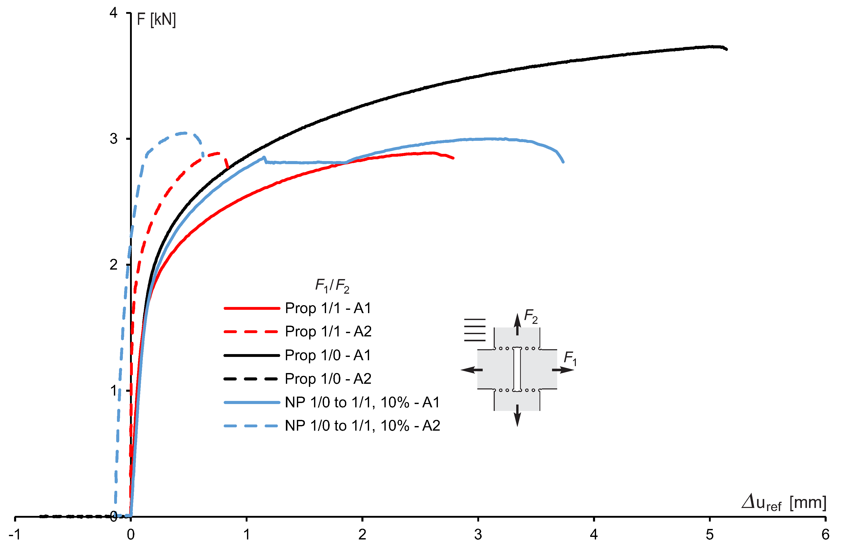
The respective thin specimens are loaded by different loading scenarios. In particular, the 0° specimen is in the first reference test simultaneously loaded by $F_1=F_2$, leading to the red load–displacement curves shown in Figure 3. Respective load–displacement curves are shown for axis 1 (Prop 1/1 - A1) and axis 2 (Prop 1/1 - A2). In this case, the maximum load is $F_1=F_2=$ 2.87 kN and the final displacement at fracture in axis 1 reaches $\Delta u_{ref.1}=$ 2.81 mm. In the second reference test, the 0° specimen is loaded by $F_1$ only (Prop 1/0 - A1 and Prop 1/0 - A2). The maximum load is $F_1=$ 3.70 kN and the final displacement at fracture is $\Delta u_{ref.1}=$ 5.11 mm. In the non-proportional loading experiment, the 0° specimen is first loaded by $F_1$ until $10\%$ of equivalent plastic strain of the second reference test has been reached in the region with holes. Then, an unloading path up to $F_1=0$ follows with subsequent loading by $F_1=F_2$. The respective blue load–displacement curves are also shown in Figure 3 for loading in axis 1 (NP 1/0 to 1/1, $10\%$ - A1) and in axis 2 (NP 1/0 to 1/1, $10\%$ - A2). For this loading history the maximum force reaches $F_1=F_2=$ 3.00 kN and the displacement at fracture is $\Delta u_{ref.1}=$ 3.73 mm. Compared with the second reference test, the non-proportional loading with pre-loading by $F_1$ leads to an increase in the maximum load of about $5\%$ and in the final displacement at fracture of $33\%$ indicating more ductile behavior caused by the pre-loading path.

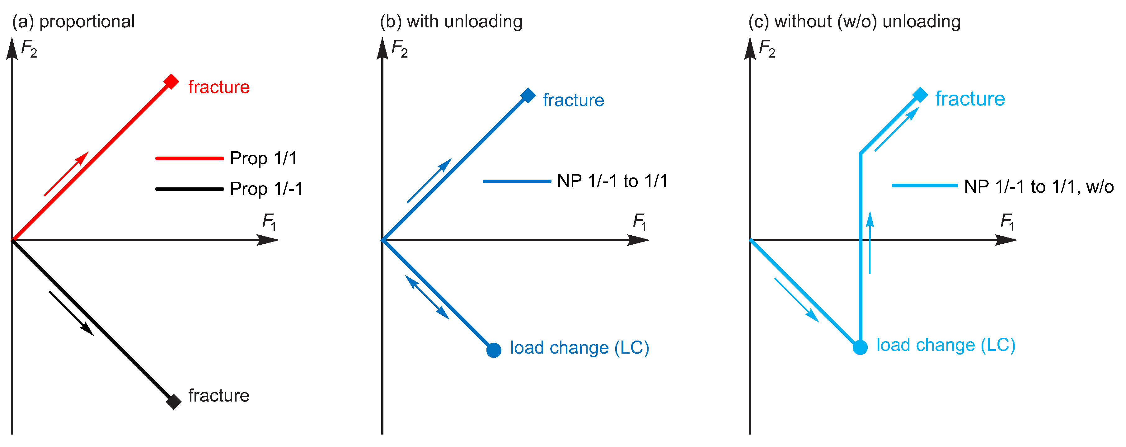
Different loading scenarios have been chosen for the 22.5° specimen, see Figure 4. In the proportional reference tests the 22.5° specimen is loaded by $F_1=F_2$ (Prop 1/1) and by $F_2=-F_1$ (Prop 1/−1), respectively (Figure 4a). In the first non-proportional experiment, the 22.5° specimen is first loaded by $F_2=-F_1$, then unloaded up to $F_1=F_2=$ 0, and in the last loading step the forces are $F_1=F_2$ (NP $1/-1$ to $1/1$; Figure 4b). In the alternative non-proportional test without unloading path (NP $1/-1$ to $1/1$, w/o; Figure 4c) the 22.5° specimen is first loaded by $F_2=-F_1$ up to the stage when $10\%$ or $20\%$ of the equivalent plastic strain of the second reference test (Prop $1/-1$) have been reached. Then, only the load $F_2$ increases until the load path of the first reference test is reached while $F_1$ stays unchanged. In the subsequent loading step, the increasing forces are $F_1=F_2$ up to final fracture.

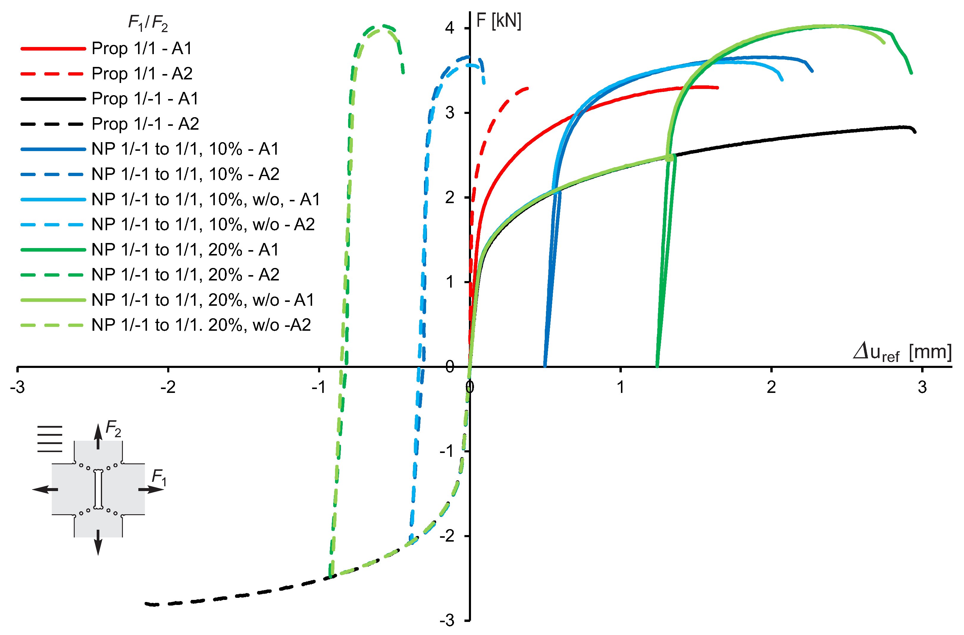
Corresponding load–displacement curves are shown in Figure 5. In the first proportional load case (Prop $1/1$), the maximum load reaches $F_1=F_2=$ 3.30 kN and the displacement at fracture is $\Delta u_{ref.1}=$ 1.60 mm. In the second proportional case (Prop 1/−1), the maximum load in axis 1 is $F_1=$ 2.42 kN and the final displacement is $\Delta u_{ref.1}=$ 2.95 mm. In the non-proportional load case with first loading by $F_2=-F_1$ up to the point of $10\%$ equivalent plastic strain and with subsequent unloading and further loading by $F_1=F_2$ (NP $1/-1$ to $1/1$, $10\%$), the maximum load is $F_1=F_2=$ 3.67 kN and the final displacement reaches $\Delta u_{ref.1}=$ 2.27 mm. This is an increase in load of $11\%$ and in the displacement of $42\%$ compared to the proportional load path with $F_1=F_2$ (Prop 1/1). In the alternative experiment without unloading path (NP $1/-1$ to $1/1$, $10\%$, w/o) the forces reach $F_1=F_2=$ 3.42 kN and the final displacement in axis 1 is $\Delta u_{ref.1}=$ 2.05 mm. These values are slightly smaller than those of the non-proportional case with the unloading step, but both non-proportional loading scenarios lead to an increase in ductility compared to the proportional reference experiment with $F_1=F_2$ (Prop $1/1$). Additional experiments have been performed where the first loading path $F_2=-F_1$ ends at the point where the maximum equivalent plastic strain reaches $20\%$. Again, loading histories with and without the unloading path are considered. In the case with the unloading path, the maximum force is $F_1=F_2=$ 4.00 kN and the final displacement reaches $\Delta u_{ref.1}=$ 2.95 mm, whereas in the loading history without the unloading path, $F_1=F_2=$ 4.00 kN and $\Delta u_{ref.1}=$ 2.75 mm are measured. These experiments clearly demonstrate that the initial pre-loading paths lead to an increase in maximum loads and final displacements at fracture and this effect is further increased by higher pre-loads.

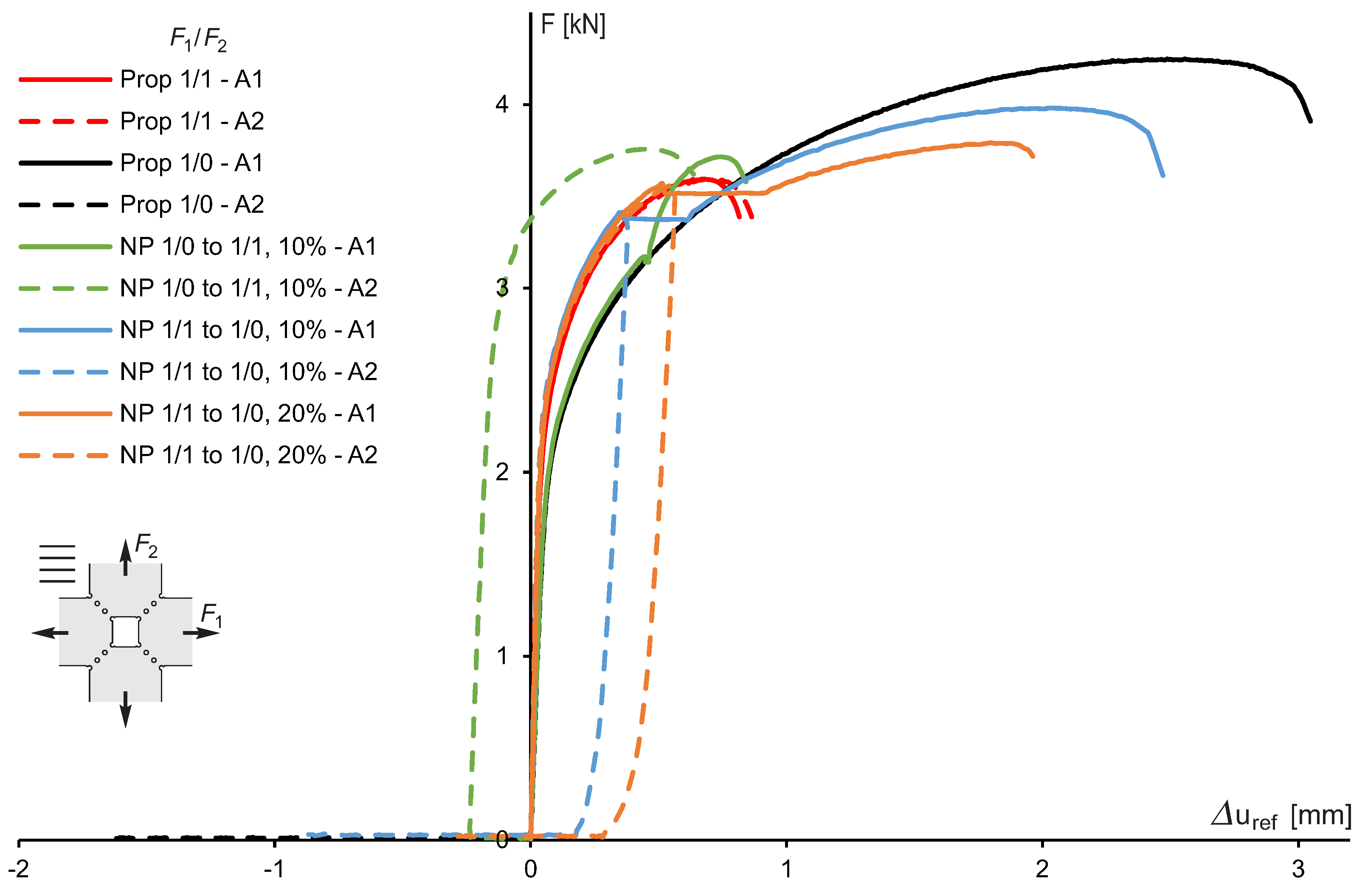
Furthermore, different proportional and non-proportional experiments have been performed with the 45° specimen and corresponding load–displacement curves are shown in Figure 6. In the first proportional reference test with the loads $F_1=F_2$ (Prop $1/1$), the maximum load is $F_1=F_2=$ 3.60 kN and the displacement at fracture reaches $\Delta u_{ref.1}=$ 0.83 mm. In the second reference experiment with uniaxial loading with $F_1$ only (Prop $1/0$), the load reaches $F_1=$ 4.38 kN and the displacement at fracture is $\Delta u_{ref.1}=$ 3.05 mm. The loading history for the first non-proportional experiment (NP 1/0 to $1/1$, $10\%$) is loading by $F_1$ only until the maximum equivalent plastic strain reaches $10\%$ of that one of the corresponding proportional test Prop $1/0$, then follows the unloading path with subsequent loading by $F_1=F_2$. In this experiment, the maximum load is $F_1=F_2=$ 3.72 kN and the final displacement reaches again $\Delta u_{ref.1}=$ 0.83 mm. Thus, compared to the reference test Prop 1/1, the load is only increased by about $9\%$, whereas the displacement at fracture remains unchanged. This means that in this case, the pre-loading step does not lead to a change in ductility. In a further non-proportional load case (NP $1/1$ to $1/0$, $10\%$), the 45° specimen is in a first step loaded by $F_1=F_2$ until the point with $10\%$ equivalent plastic strain has been reached. After unloading, the specimen is further loaded by $F_1$ up to final fracture. In this experiment, the load reaches $F_1=$ 4.00 kN and the final displacement in axis 1 at fracture is $\Delta u_{ref.1}=$ 2.45 mm. Compared to the proportional reference test Prop 1/0, the decrease in load is of about $9\%$ and in the displacement of $20\%$ what means that in this case the pre-loading step leads to more brittle behavior. Alternatively, this loading history is again considered but in the first step the loads $F_1=F_2$ stop when the equivalent plastic strain reaches $20\%$. This leads to the maximum force $F_1=$ 3.75 kN and the fracture displacement in axis 1 is $\Delta u_{ref.1}=$ 1.94 mm. Thus, this pre-loading step with higher forces leads to a further decrease in ductility with a $15\%$ smaller load and $36\%$ smaller displacement.

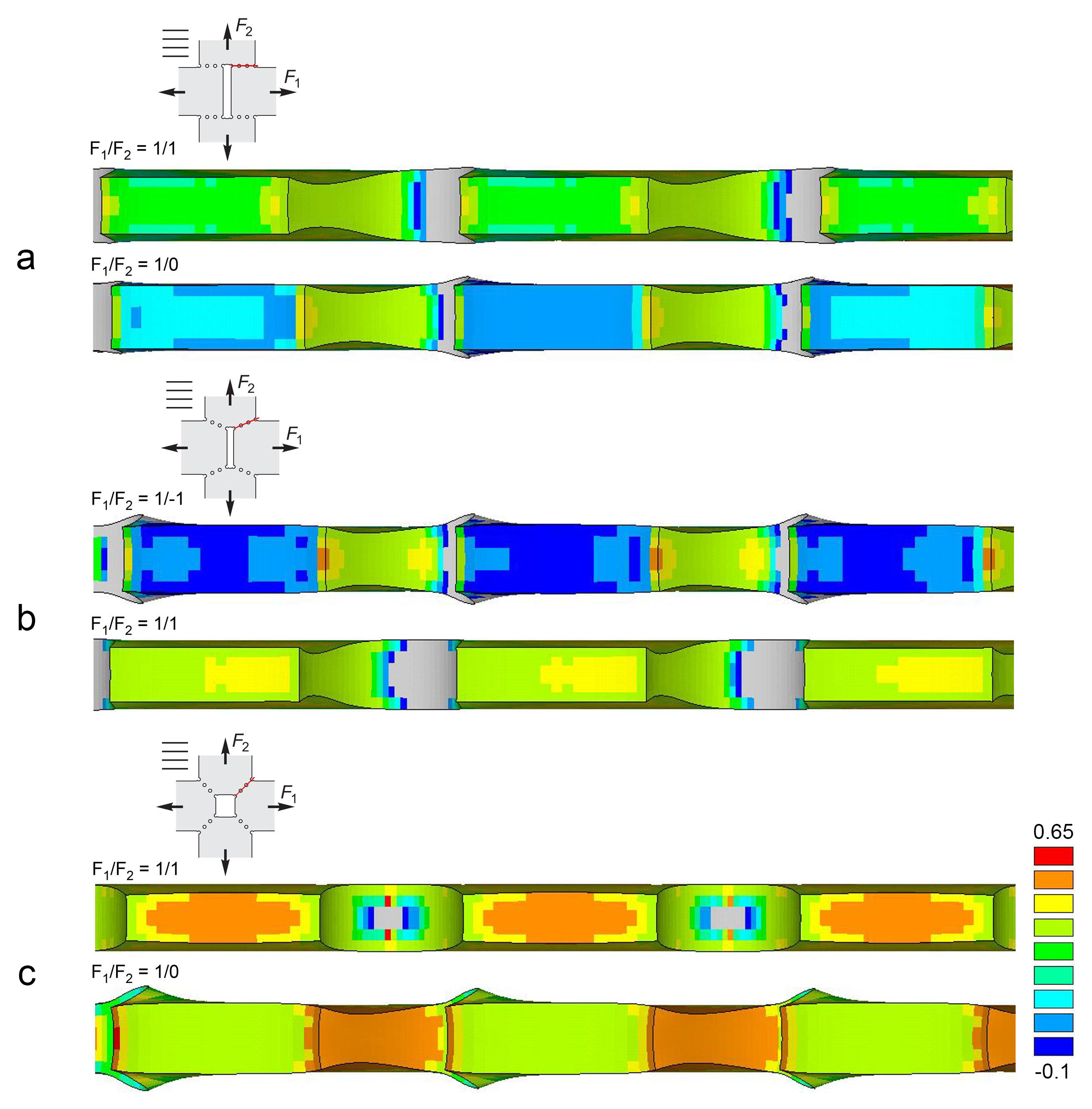
In order to analyze the stress states in the critical areas between the holes, numerical simulation of the respective experiments has been performed. The finite element program ANSYS has been used and the calculations are based on Voce hardening and Hill’s yield criterion [35] for the investigated anisotropic aluminum alloy. All determined elastic and plastic material parameter are given in

Table 2. Material parameters used for numerical simulation of aluminum alloy AA6016-T4, 1 mm.

$K\left[MPa\right]$	$E\left[MPa\right]$	$c_0\left[MPa\right]$	$R_0\left[MPa\right]$	$R_{\infty }\left[MPa\right]$	$b\left[-\right]$	$r_{0°}$	$r_{45°}$	$r_{90°}$
57,500	69,000	155	260	130	16	0.6827	0.4369	0.6333
$F\left[-\right]$	$G\left[-\right]$	$H\left[-\right]$	$L\left[-\right]$	$M\left[-\right]$	$N\left[-\right]$
1.3619	1.1885	0.8114	3	3	2.3267

, for details on the procedure and equations see [27]. Furthermore, the corresponding Lankford coefficients are given in Table 2. The numerically predicted stress triaxialities $\eta ={\sigma }_m/{\sigma }_{eq}$, with the mean stress ${\sigma }_m$ and the equivalent von Mises stress ${\sigma }_{eq}$, are shown in Figure 7 for the different specimens at the red marked cross section. The scale in Figure 7 was chosen according to the values occurring in the cut areas of the cross-section relevant for the analysis here, and the gray areas outside this scale are located in parts of the specimen without major inelastic deformations. In particular, for the 0° specimen, the proportional load case $F_1/F_2=1/1$ leads to shear behavior caused by $F_1$ with superimposed tension due to $F_2$. In this case, nearly homogeneous stress states occur in the areas of the connectors with $\eta =$ 0.30. If this specimen is only loaded by $F_1$, shear behavior occurs with the stress triaxiality $\eta =$ 0.00 in the area of the middle connector and $\eta =$ 0.05 in the outer ones. And the distribution of the stress triaxialities in these areas is again nearly homogeneous. In addition, the stress state of the 22.5° specimen is numerically predicted. For the load case $F_1/F_2=1/-1$, very small stress triaxialities occur in the middle of the areas of the connectors with $\eta =$−0.10 and slightly larger value at the boundaries of these areas. Due to these loads, there is shear behavior with small tension effects caused by $F_1$, which is superimposed by remarkable compression caused by $F_2$, leading to these negative stress triaxialities. For the load ratio $F_1/F_2=1/1$ in the 22.5° specimen, stress triaxialities of $\eta =$ 0.40 are reached on the right part of the connectors, whereas they are $\eta =$ 0.35 on the left side. Compared to the 0° specimen, which shows for this load ratio nearly homogeneous distribution with $\eta =$ 0.30, the geometry with 22.5° arrangement of holes leads to higher stress triaxialities and to a less homogeneous distribution, see Figure 7b. Furthermore, the 45° specimen has been numerically analyzed for two different load ratios. The load ratio $F_1/F_2=1/1$ leads to remarkably high stress triaxialities with maxima $\eta =$ 0.60 in the center of the connectors with less homogeneous distribution. These high stress triaxialities are caused by tensile loading in two directions. Thus, different values and distributions of stress triaxialities are obtained for the same load ratio $F_1/F_2=1/1$ only caused by the arrangement of the holes. For the load ratio $F_1/F_2=1/0$, nearly homogeneous distribution of the stress triaxiality is numerically predicted with $\eta =$ 0.33. The numerical analysis clearly shows that with these three geometries with different arrangements of the holes in the central part and different load ratios, the effect of a wide range of stress triaxialities on deformation and failure behavior can be investigated, see also

Table 3. Overview of stress triaxiality $\eta$ for different geometries and loading ratios $F_1/F_2$, indicated with one decimal place.

0°
$F_1/F_2$	$1/1$	$1/0$
$\eta$	0.3	0.0
22.5°
$F_1/F_2$	$1/-1$	$1/1$
$\eta$	$-0.1$	0.4
45°
$F_1/F_2$	$1/1$	$1/0$
$\eta$	0.6	0.3

for an overview.

During the respective experiments, the strain fields in the critical parts of the specimens with holes have been monitored and evaluated by digital image correlation (DIC). Calculation of the principal strains at the center of the middle connector leads to the major strain–minor strain curves shown in Figure 8. In the diagrams, the evolution of the strains for the reference experiments with proportional load paths with nearly straight lines are shown. The evolution of the strains for the non-proportional loading histories are between these lines. They start on the reference line, and after a change in the load path they move to the other reference line. In Figure 8b, it can be clearly seen that there is no remarkable difference between the principal strains measured in experiments with and without an unloading path, indicating that at the point of load change the irreversible strains are predominant and the elastic ones are marginal.

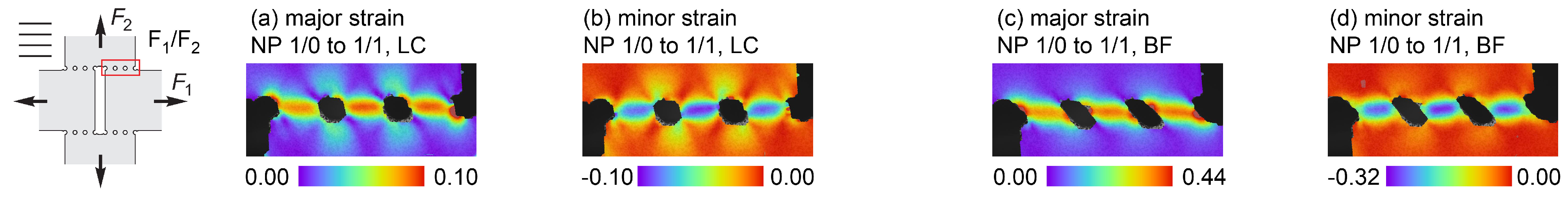
The distribution of major and minor strain fields in the critical part of the 0° specimen (framed region) during and at the end of the non-proportional experiments, evaluated by DIC is shown in Figure 9. In particular, at the end of the first load step $F_1/F_2=1/0$ (LC) localization of the principal strains can be seen between the holes in the framed section of the specimen. The major strain reaches ${ϵ}_1=0.10$ and the minor strain is ${ϵ}_2=-0.10$. After unloading and subsequent loading with $F_1/F_2=1/1$ the principal strains remarkably increase, and at the end of the non-proportional loading scenario (BF) the major strain reaches ${ϵ}_1=0.44$ and the minor strain is ${ϵ}_2=-0.32$, again localized in small bands between the holes. This strongly localized behavior indicates that damage and fracture will occur in these bands, leading to the final fracture of the specimen.

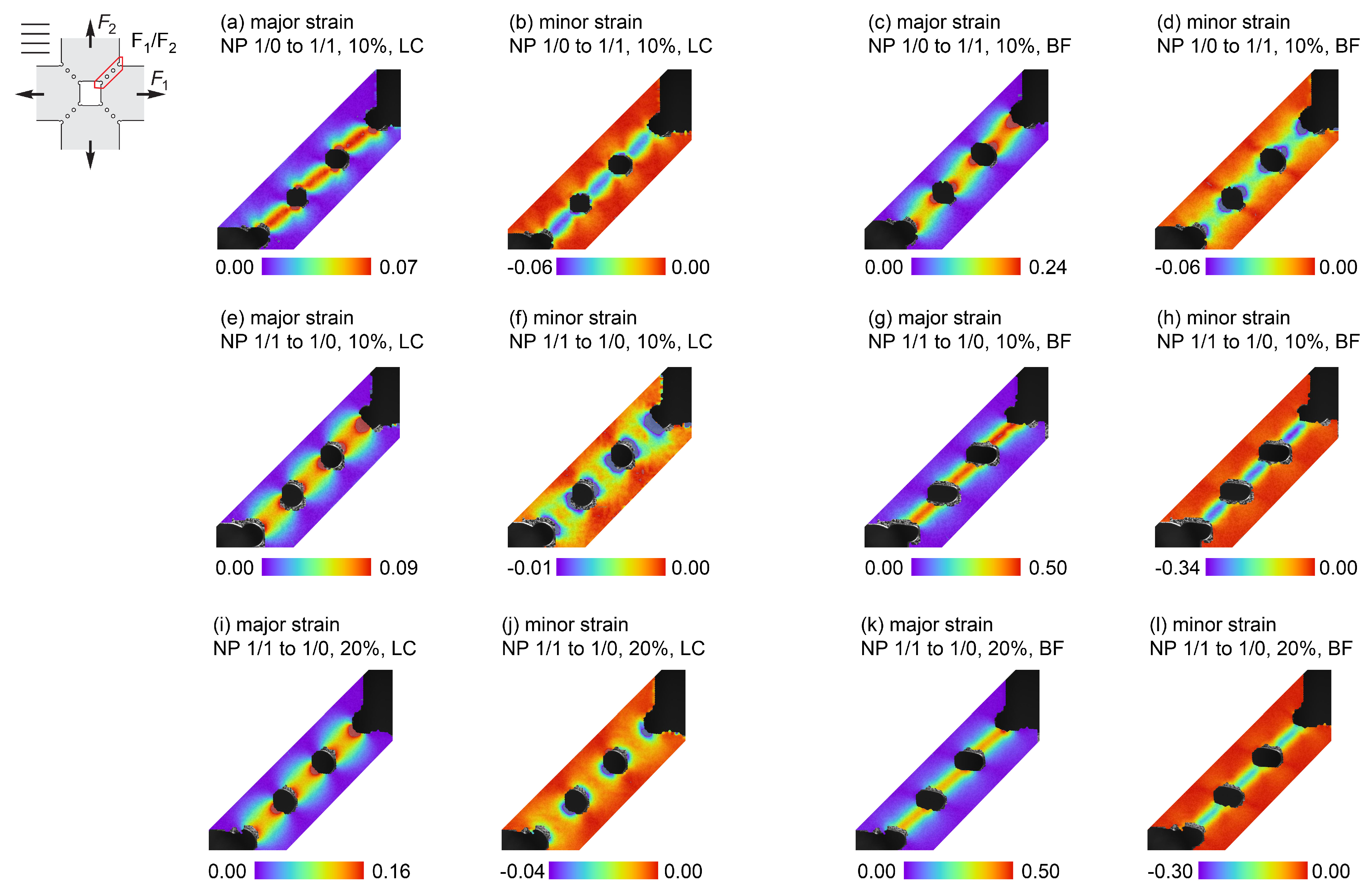
Furthermore, Figure 10 shows the experimentally evaluated principal strain fields in the framed region of the 22.5° specimen for different non-proportional loading histories. In the case NP $1/-1$ to 1/1, $10\%$, the principal strains after the first load path (LC) are again localized in bands between the holes. The major strain is ${ϵ}_1=$ 0.08 and the minor strain is ${ϵ}_2=-0.10$. After unloading and subsequent loading with $F_1/F_2=1/1$ the principal strains increase and at the end of the non-proportional loading scenario (BF) the major strain reaches ${ϵ}_1=0.33$ and the minor strain is ${ϵ}_2=-0.15$. It can be seen in Figure 10c that the maximum of the major strain is concentrated in small points at the boundaries of the holes but a localized band is not visible. On the other hand the distribution of the minor strain shows a localized band (Figure 10d) but the absolute values are not very high. These strain fields indicate that fracture will be initiated at the boundaries of the holes where high principal strains have been measured but the fracture line must not be straight. In the alternative experiment the specimen was not unloaded after the first step with $F_1/F_2=1/-1$ and after this first load path the force $F_2$ was increased until it reached $F_1=F_2$ followed by the last load step with $F_1/F_2=1/1$. The corresponding strain fields are shown in Figure 10e–h. At the end of this experiment, the major strain reaches ${ϵ}_1=$ 0.30 and the minor strain is ${ϵ}_2=-0.15$ but in contrast to the history with unloading path (Figure 10a–d) the principal strains are more localized in a band. In addition, these tests have also been driven with a load change when $20\%$ of the equivalent plastic strain compared to the corresponding proportional load path have been reached. Experimental results are shown in Figure 10i–l for the loading history with unloading path and in Figure 10m–p for the test without unloading. This leads to an increase in the absolute values of the principal strains after the first load path $F_1/F_2=1/-1$ where the major strain reaches ${ϵ}_1=0.19$ and the minor strain is ${ϵ}_2=-0.22$. After unloading and reloading with $F_1/F_2=1/1$, the major strain is ${ϵ}_1=0.31$ and the minor strain is ${ϵ}_2=-0.22$. Compared to the loading history with load change at $10\%$ equivalent plastic strain (Figure 10c,d) there is no remarkable change in the distribution and amount of the principal strains. Similar behavior is observed in the case without unloading. The major strain reaches ${ϵ}_1=0.31$ and the minor strain is ${ϵ}_2=-0.22$, and, again, compared to the loading history with load change at $10\%$ equivalent plastic strain (Figure 10g,h) there is no remarkable change in the distribution and amount of the principal strains.

Moreover, the distribution of experimentally obtained principal strain fields in the framed region of the 45° specimen are shown for three different loading histories in Figure 11. In particular, in the case NP $1/0$ to $1/1$, $10\%$, after the first load path (LC) the major strain reaches ${ϵ}_1=0.07$ and the minor strain is ${ϵ}_2=-0.06$. The major strains are localized between the holes in a small band with a slight S-shape. After unloading and reloading with $F_1/F_2=1/1$, the major strain increases, whereas the minimum of the minor strain remains nearly unchanged. The maxima of the major strain are concentrated at the boundaries of the holes, but the distribution of the minor strain is more diffuse. Based on these results, it is difficult to propose the fracture mode. In the further experiment NP $1/1$ to $1/0$, $10\%$ (Figure 11e–h), after the first load path $F_1=F_2$ the major strain is ${ϵ}_1=$ 0.09 and the minor strain is only ${ϵ}_2=-0.01$ with the concentration of the extrema at the boundaries of the holes, and sharp localized bands are not visible. After unloading and reloading only with $F_1$, the major strain reaches ${ϵ}_1=0.50$ and the minor strain is ${ϵ}_2=-0.34$ with remarkably localized straight bands between the holes. This behavior indicates that straight fracture lines between the holes are expected. In the experiment with load change at the point of $20\%$ of the equivalent plastic strain measured in the reference test (Figure 11i–l), after the first load path, the major strain is ${ϵ}_1=$ 0.16 and the minor strain is ${ϵ}_2=-0.04$ but, again, only with the concentration of the extrema at the boundaries of the holes. After unloading and reloading only with $F_1$, the major strain is ${ϵ}_1=0.50$ and the minor strain reaches ${ϵ}_2=-0.30$, again with remarkably localized straight bands between the holes. This behavior also indicates that straight fracture lines between the holes are expected to occur.

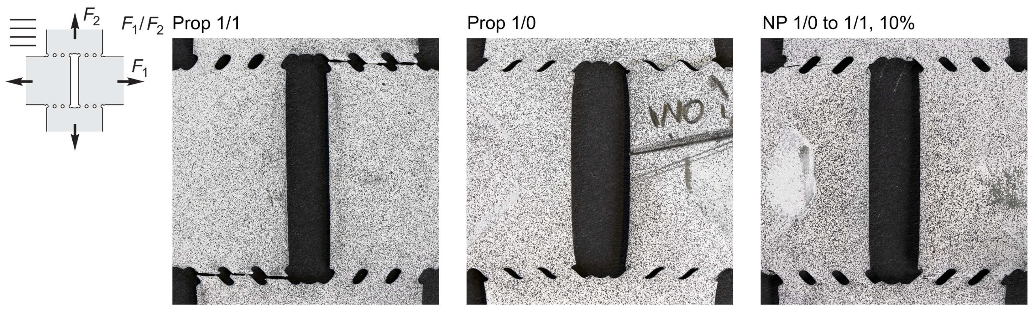
After the experiments, photos of the fractured specimens are taken to show the fracture modes. In particular, photos of the 0° specimen are shown in Figure 12. For proportional loading with $F_1=F_2$ (Prop $1/1$), shear deformation superimposed by tension occurs in the critical region of the specimen. This leads to the shearing and elongation of the holes. The fracture mode is a straight line between the holes. In the case of proportional loading by $F_1$ (Prop 1/0) shear mechanisms occur in the critical region of the specimen leading to remarkable shearing of the holes. Straight fracture lines can be seen between the top and bottom of the holes corresponding to the distribution of major strain shown in Figure 9a. At the end of the non-proportional loading history NP 1/0 to 1/1, $10\%$, combination of shear deformation and tensile elongation of the holes with straight horizontal fracture lines is visible in Figure 12. This failure behavior was predicted by the major strain distribution shown in Figure 9c,d.

Furthermore, the fracture modes for the 22.5° specimen are shown in Figure 13. In particular, for the proportional load case with $F_1=F_2$ (Prop $1/1$) growth of the holes with elongation in diagonal direction can be seen in Figure 13 and the fracture mode is characterized by lines with slight S-shape between the middle of the holes. In the other proportional test with $F_2=-F_1$ (Prop $1/-1$), the holes are sheared and straight fracture lines occur between the bottom and top of the holes. This behavior corresponds to the localized band of the major strain shown in Figure 10a. After the non-proportional test NP $1/-1$ to $1/1$, $10\%$, shearing and elongation in diagonal direction of the holes occur and the fracture is characterized by S-shaped fracture lines between the middle of the holes. This behavior is observed for load histories with and without unloading, and nicely corresponds to the distribution of the major strain fields shown in Figure 10c,g. Similar deformation and failure behavior can be seen after the non-proportional experiments (NP $1/-1$ to $1/1$, $20\%$ and NP $1/-1$ to $1/1$, $20\%$, w/o) where the first load step ends at points with $20\%$ of the equivalent plastic strain of the respective proportional test.

Moreover, Figure 14 shows the fracture modes for the 45° specimen for different loading scenarios. For proportional loading with $F_1=F_2$ (Prop $1/1$), the holes are grown, caused by the high stress triaxialities shown in Figure 7c and elongated in diagonal direction shortly before fracture by straight lines occurs. After the second proportional experiment with the 45° specimen loaded only by $F_1$ (Prop $1/0$), the elongation of the holes in the loading direction is visible and nearly straight fracture lines occur corresponding to the major strain field shown in Figure 11a. In the non-proportional case NP $1/0$ to $1/1$, 10, the failure behavior is similar to that one observed in the proportional experiment Prop $1/1$. This means that the fracture mode is nearly unaffected by the first load path and only the final loading up to fracture dominates the fracture mode, here with growth of the holes and nearly straight fracture lines. After the alternative non-proportional tests (NP $1/1$ to $1/0$, $10\%$, and NP $1/1$ to $1/0$, $20\%$) the holes show elongation in final loading direction with straight failure lines corresponding to the localization of the major strains in small bands, see Figure 11g,k.

After the respective experiments the fracture surfaces have been analyzed by scanning electron microscopy (SEM) to elucidate the stress-state-dependent damage and fracture modes of the thin specimens. For the 0° specimen the photos of the fracture surfaces are shown in Figure 15. For the proportional loading with $F_1=F_2$ the stress triaxiality $\eta =0.27$ has been numerically predicted, see Figure 7a. This leads to void growth with combined shearing of the pores which can be clearly seen in the SEM image. In the case of the alternative proportional loading Prop $1/0$ shear mechanisms occur corresponding to the numerically predicted stress triaxiality $\eta =0.00$ (Figure 7a). This leads to predominant shear-cracks on the micro-scale with only very small pre-existing voids which are also sheared. In the combined non-proportional loading history NP $1/0$ to $1/1$, $10\%$, shear mechanisms are pre-dominant in the first load path which are then superimposed by shear-tension loading leading to shear-cracks and small voids, but compared to the path Prop $1/1$ the voids are smaller due to the first load path. Thus, concerning the damage and fracture processes on the micro-level the first load step has an influence.

SEM images of fracture surfaces for the 22.5° specimen are shown in Figure 16. After the proportional load path with $F_1=F_2$ (Prop $1/1$), many voids with different sizes can be seen as well as some shear-cracks. This damage and fracture behavior on the micro-level corresponds to the numerically predicted stress triaxiality $\eta =0.40$, see Figure 7b. In the case of proportional loading with the load ratio $F_2=-F_1$ (Prop $1/-1$), remarkable shear-cracks can be seen in the SEM image with only few very small voids, which is typical for the negative stress triaxialities $\eta =-0.10$ predicted in the numerical analysis, see Figure 7b. After the corresponding non-proportional loading histories (NP $1/-1$ to $1/1$, $10\%$ and NP $1/-1$ to $1/1$, $10\%$, w/o), the main damage process is formation of micro-shear-cracks with later growth of voids, which compared to the proportional path with $F_1=F_2$ remain small. This can be observed in the loading histories with and without unloading path. The effect of the first load path on damage can be seen in the SEM images after the experiments with first loading up to the point with $20\%$ of the equivalent plastic strain of the reference test. Compared to the $10\%$ cases, the voids are smaller, caused by the shear mechanisms in the first step. Also, in these pictures, the effect of the first load path on damage and fracture on the micro-scale can be seen.

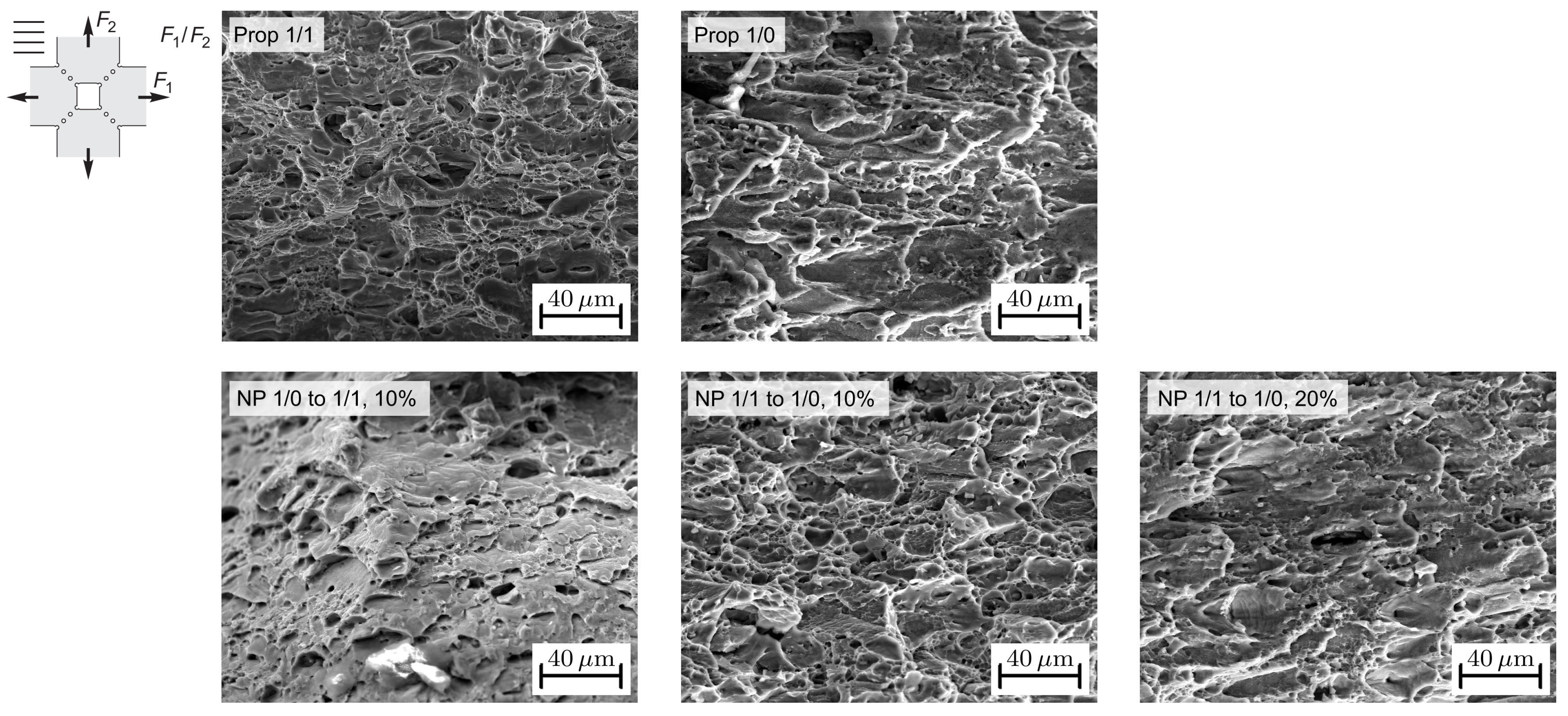
For the 45° specimen, respective fracture surfaces can be studied in Figure 17. For proportional loading Prop $1/1$, the remarkable growth of voids can be seen in the SEM images corresponding to high-stress triaxialities up to $\eta =0.60$. These voids are the largest compared to all other tests discussed above and nearly no shear effects are visible. However, after proportional loading Prop 1/0, a combination of voids and shear-cracks can be seen in the photos, which is typical for the stress triaxiality $\eta =0.33$. After the non-proportional case with first loading by $F_1$, only followed by unloading and final loading with $F_1=F_2$ up to fracture (NP $1/0$ to $1/1$, $10\%$), shear mechanisms with superimposed large voids can be seen in the photo and it seems that the shear-cracks failed under subsequent tension. Compared to the corresponding proportional path Prop 1/1, the shear effect of the first load path is clearly visible. In addition, the specimen has been tested with NP $1/1$ to $1/0$, $10\%$, showing many small voids and shear mechanisms, but compared to the corresponding proportional path Prop 1/0, there are more and larger voids. This effect can also be seen after loading NP 1/1 to $1/0$, $20\%$, with larger voids. Therefore, these loading cases for the 45° specimen also confirm that the loading history has a remarkable influence on the damage and fracture processes on the micro-level, leading to different failure modes.

4. Conclusions

In this paper, the effect of the load path on the damage and fracture behavior of thin metal sheets has been analyzed in detail. Experiments with newly designed biaxially loaded specimens have been performed with focus on non-proportional loading histories. The main conclusions are:

• The characterization of ductile metals is recommended to be based on an enhanced experimental program, including biaxial tests with different non-proportional load paths to detect the effect of stress state and stress history on deformation, damage, and fracture behavior.
• In specimens taken from thin metal sheets, bands of holes can be used to localize inelastic deformations and damage in desired critical regions.
• Different non-proportional load paths influence the load–displacement behavior. They affect the maximum loads and the displacement at fracture. First, tensile loading leads to more brittle behavior, whereas more ductile behavior is observed with the shear-dominated stress state in the first load step.
• The final stresses remain nearly unaffected by the loading histories although the stress paths are different.
• Changes in the amount, width and orientation of localized principal strain bands occur as a result of different load paths.
• Damage and fracture processes on the micro-scale are influenced by the load path, leading to the accumulation of all stress-state-dependent damage processes.
• The experimental results deliver important information on damage and fracture processes during non-proportional load paths. They can be used to develop and to validate constitutive models.

References

1. Becker, R.; Needleman, A.; Richmond, O.; Tvergaard, V. Void growth and failure in notched bars. J. Mech. Phys. Solids 1988, 36, 317–351. [Google Scholar] [CrossRef]
2. Bao, Y.; Wierzbicki, T. On fracture locus in the equivalent strain and stress triaxiality space. Int. J. Mech. Sci. 2004, 46, 81–98. [Google Scholar] [CrossRef]
3. Bonora, N.; Gentile, D.; Pirondi, A.; Newaz, G. Ductile damage evolution under triaxial state of stress: Theory and experiments. Int. J. Plast. 2005, 21, 981–1007. [Google Scholar] [CrossRef]
4. Bai, Y.; Wierzbicki, T. A new model of metal plasticity and fracture with pressure and Lode dependence. Int. J. Plast. 2008, 24, 1071–1096. [Google Scholar] [CrossRef]
5. Brünig, M.; Chyra, O.; Albrecht, D.; Driemeier, L.; Alves, M. A ductile damage criterion at various stress triaxialities. Int. J. Plast. 2008, 24, 1731–1755. [Google Scholar] [CrossRef]
6. Gao, X.; Zhang, G.; Roe, C. A study on the effect of the stress state on ductile fracture. Int. J. Damage Mech. 2010, 19, 75–94. [Google Scholar] [CrossRef]
7. Driemeier, L.; Brünig, M.; Micheli, G.; Alves, M. Experiments on stress-triaxiality dependence of material behavior of aluminum alloys. Mech. Mater. 2010, 42, 207–217. [Google Scholar] [CrossRef]
8. Dunand, M.; Mohr, D. On the predictive capabilities of the shear modified Gurson and the modified Mohr–Coulomb fracture models over a wide range of stress triaxialities and Lode angles. J. Mech. Phys. Solids 2011, 59, 1374–1394. [Google Scholar] [CrossRef]
9. Roth, C.C.; Mohr, D. Ductile fracture experiments with locally proportional loading histories. Int. J. Plast. 2016, 79, 328–354. [Google Scholar] [CrossRef]
10. Roth, C.C.; Morgeneyer, T.F.; Cheng, Y.; Helfen, L.; Mohr, D. Ductile damage mechanism under shear-dominated loading: In-situ tomography experiments on dual phase steel and localization analysis. Int. J. Plast. 2018, 109, 169–192. [Google Scholar] [CrossRef]
11. Lou, Y.; Chen, L.; Clausmeyer, T.; Tekkaya, A.E.; Yoon, J.W. Modeling of ductile fracture from shear to balanced biaxial tension for sheet metals. Int. J. Solids Struct. 2017, 112, 169–184. [Google Scholar] [CrossRef]
12. Haji Aboutalebi, F.; Poursina, M.; Nejatbakhsh, H.; Khataei, M. Numerical simulations and experimental validations of a proposed ductile damage model for DIN1623 St12 steel. Eng. Fract. Mech. 2018, 192, 276–289. [Google Scholar] [CrossRef]
13. Demmerle, S.; Boehler, J.P. Optimal design of biaxial tensile cruciform specimens. J. Mech. Phys. Solids 1993, 41, 143–181. [Google Scholar] [CrossRef]
14. Lin, S.B.; Ding, J.L. Experimental study of the plastic yielding of rolled sheet metals with the cruciform plate specimen. Int. J. Plast. 1995, 11, 583–604. [Google Scholar] [CrossRef]
15. Müller, W.; Pöhlandt, K. New experiments for determining yield loci of sheet metal. J. Mater. Process. Technol. 1996, 60, 643–648. [Google Scholar] [CrossRef]
16. Green, D.E.; Neale, K.W.; MacEwen, S.R.; Makinde, A.; Perrin, R. Experimental investigation of the biaxial behaviour of an aluminum sheet. Int. J. Plast. 2004, 20, 1677–1706. [Google Scholar] [CrossRef]
17. Kuwabara, T. Advances in experiments on metal sheets and tubes in support of constitutive modeling and forming simulations. Int. J. Plast. 2007, 23, 385–419. [Google Scholar] [CrossRef]
18. Kulawinski, D.; Nagel, K.; Henkel, S.; Hübner, P.; Fischer, H.; Kuna, M.; Biermann, H. Characterization of stress–strain behavior of a cast TRIP steel under different biaxial planar load ratios. Eng. Fract. Mech. 2011, 78, 1684–1695. [Google Scholar] [CrossRef]
19. Brünig, M.; Brenner, D.; Gerke, S. Modeling of Stress-State-Dependent Damage and Failure of Ductile Metals. Appl. Mech. Mater. 2015, 784, 35–42. [Google Scholar] [CrossRef]
20. Song, X.; Leotoing, L.; Guines, D.; Ragneau, E. Characterization of forming limits at fracture with an optimized cruciform specimen: Application to DP600 steel sheets. Int. J. Mech. Sci. 2017, 126, 35–43. [Google Scholar] [CrossRef]
21. Gerke, S.; Zistl, M.; Bhardwaj, A.; Brünig, M. Experiments with the X0-specimen on the effect of non-proportional loading paths on damage and fracture mechanisms in aluminum alloys. Int. J. Solids Struct. 2019, 163, 157–169. [Google Scholar] [CrossRef]
22. Zhang, W.; Zhu, Z.; Zhou, C.; He, X. Biaxial Tensile Behavior of Commercially Pure Titanium under Various In-Plane Load Ratios and Strain Rates. Metals 2021, 11, 155. [Google Scholar] [CrossRef]
23. Brünig, M.; Koirala, S.; Gerke, S. Analysis of damage and failure in anisotropic ductile metals based on biaxial experiments with the H-specimen. Exp. Mech. 2022, 62, 183–197. [Google Scholar] [CrossRef]
24. Hou, Y.; Lee, M.G.; Lin, J.; Min, J. Experimental characterization and modeling of complex anisotropic hardening in quenching and partitioning (Q&P) steel subject to biaxial non-proportional loadings. Int. J. Plast. 2022, 156, 103347. [Google Scholar] [CrossRef]
25. Raj, A.; Verma, R.K.; Singh, P.K.; Shamshoddin, S.; Biswas, P.; Narasimhan, K. Experimental and numerical investigation of differential hardening of cold rolled steel sheet under non-proportional loading using biaxial tensile test. Int. J. Plast. 2022, 154, 103297. [Google Scholar] [CrossRef]
26. Kong, X.; Chen, J.; Madi, Y.; Missoum-Benziane, D.; Besson, J.; Morgeneyer, T. Plasticity and ductility of an anisotropic recrystallized AA2198 Al-Cu-Li alloy in T3 and T8 conditions during proportional and non-proportional loading paths: Simulations and experiments. J. Theor. Comput. Appl. Mech. 2023, 1–31. [Google Scholar] [CrossRef]
27. Gerke, S.; Valencia, F.R.; Norz, R.; Volk, W.; Brünig, M. Damage and fracture in thin metal sheets: New biaxial experiments. Adv. Ind. Manuf. Eng. 2023, 7, 100129. [Google Scholar] [CrossRef]
28. Wang, J.; Chow, C.L. Mixed Mode Ductile Fracture Studies With Nonproportional Loading Based on Continuum Damage Mechanics. J. Eng. Mater. Technol. 1989, 111, 204–209. [Google Scholar] [CrossRef]
29. Chow, C.L.; Lu, T.J. An analytical and experimental study of mixed-mode ductile fracture under nonproportional loading. Int. J. Damage Mech. 1992, 1, 191–236. [Google Scholar] [CrossRef]
30. Basu, S.; Benzerga, A.A. On the path-dependence of the fracture locus in ductile materials: Experiments. Int. J. Solids Struct. 2015, 71, 79–90. [Google Scholar] [CrossRef]
31. Cortese, L.; Nalli, F.; Rossi, M. A nonlinear model for ductile damage accumulation under multiaxial non-proportional loading conditions. Int. J. Plast. 2016, 85, 77–92. [Google Scholar] [CrossRef]
32. Zhuang, X.; Wang, T.; Zhu, X.; Zhao, Z. Calibration and application of ductile fracture criterion under non-proportional loading condition. Eng. Fract. Mech. 2016, 165, 39–56. [Google Scholar] [CrossRef]
33. Gerke, S.; Zistl, M.; Brünig, M. Experiments and numerical simulation of damage and fracture of the X0-specimen under non-proportional loading paths. Eng. Fract. Mech. 2020, 224, 106795. [Google Scholar] [CrossRef]
34. Brünig, M.; Zistl, M.; Gerke, S. Numerical analysis of experiments on damage and fracture behavior of differently preloaded aluminum alloy specimens. Metals 2021, 11, 381. [Google Scholar] [CrossRef]
35. Hill, R. A theory of the yielding and plastic flow of anisotropic metals. Proc. R. Soc. Lond. Ser. A Math. Phys. Sci. 1948, 193, 281–297. [Google Scholar] [CrossRef]
Figure 1. Specimen geometries for non-proportional loading: (a) notation, (b,c) photo of central part 0° and 45°, (d) photo of complete specimen 22.5°, and (eg) detailed sketch of central part (all measures in [mm]).
Metals 14 00397 g001
Figure 2. Experimental setup and downholder: (a) overall setup including DIC system and open downholder, (b) closed downholder in biaxial setup and (c) sketch of downholder.
Metals 14 00397 g002
Figure 3. Load –displacement curves of different proportional (Prop) and non-proportional Load (NP) cases of the 0° specimen; solid lines (A1) refer to Δ u r e f . 1 and dashed lines (A2) to Δ u r e f . 2 as defined in Equation (2).
Metals 14 00397 g003
Figure 4. Loading histories for the 22.5° specimen.
Metals 14 00397 g004
Figure 5. Load–displacement curves of different proportional (Prop) and non-proportional load (NP) cases of the 22.5° specimen; solid lines (A1) refer to Δ u r e f . 1 and dashed lines (A2) to Δ u r e f . 2 as defined in Equation (2).
Metals 14 00397 g005
Figure 6. Load–displacement curves of different proportional (Prop) and non-proportional load (NP) cases of the 45° specimen; solid lines (A1) refer to Δ u r e f . 1 and dashed lines (A2) to Δ u r e f . 2 as defined in Equation (2).
Metals 14 00397 g006
Figure 7. Numerically calculated stress triaxiality η for different loading ratios for the (a) 0° specimen, (b) 22.5° specimen and (c) 45° specimen.
Metals 14 00397 g007
Figure 8. Experimentally obtained evolution of major and minor strains at the center of the middle connector for the (a) 0° specimen, (b) 22.5° specimen and (c) 45° specimen.
Metals 14 00397 g008
Figure 9. Experimentally obtained major and minor strains at load change (LC) and before fracture (BF) for the 0° geometry under non-proportional loading.
Metals 14 00397 g009
Figure 10. Experimentally obtained major and minor strains at load change (LC) and before fracture (BF) for the 22.5° geometry under non-proportional loading.
Metals 14 00397 g010
Figure 11. Experimentally obtained major and minor strains at load change (LC) and before fracture (BF) for the 45° geometry under non-proportional loading.
Metals 14 00397 g011
Figure 12. Photos of the fractured specimens of 0° geometry for different proportional and non-proportional load cases.
Metals 14 00397 g012
Figure 13. Photos of the fractured specimens of 22.5° geometry for different proportional and non-proportional load cases.
Metals 14 00397 g013
Figure 14. Photos of the fractured specimens of 45° geometry for different proportional and non-proportional load cases.
Metals 14 00397 g014
Figure 15. SEM images of fracture surfaces of the 0° specimen for different proportional and non-proportional load cases.
Metals 14 00397 g015
Figure 16. SEM images of fracture surfaces of the 22.5° specimen for different proportional and non-proportional load cases.
Metals 14 00397 g016
Figure 17. SEM images of fracture surfaces of the 45° specimen for different proportional and non-proportional load cases.
Metals 14 00397 g017