Article

Theoretical Study on Thermal Stresses of Metal Bars with Different Moduli in Tension and Compression

1
School of Civil Engineering, Chongqing University, Chongqing 400045, China
2
Key Laboratory of New Technology for Construction of Cities in Mountain Area (Chongqing University), Ministry of Education, Chongqing 400045, China
*
Author to whom correspondence should be addressed.
Metals 2022, 12(2), 347; https://doi.org/10.3390/met12020347
Submission received: 21 January 2022 / Revised: 10 February 2022 / Accepted: 14 February 2022 / Published: 16 February 2022
(This article belongs to the Special Issue Thermo-Physical Properties of Metals and Oxides)

Abstract

:
Extensive studies have shown that engineering materials, including metals and their oxides, will present different mechanical properties in tension or compression; however, this difference is generally neglected due to the complexity of the analysis. In this study, we theoretically analyze the thermal stress of a metal bar with a bimodular effect. First, the common strain suppression method is used to obtain a one-dimensional thermal stress expression. As a contrast with the one-dimensional solution, a two-dimensional thermoelasticity solution is also derived, based on the classical Duhamel theorem concerning body force analogy. Results indicate an important phenomenon that the linear temperature rise mode will produce thermal stress in a bimodular metal bar, whereas there is no thermal stress in the case of singular modulus. If the equilibrium relation is needed to be satisfied, the variation trend between different moduli and different thermal expansion coefficients in tension and compression should be opposite. In addition, the amplitude of stress variation, from the maximum tensile stress to the maximum compressive stress, increases dramatically. There exists an inevitable link between one- and two-dimensional solutions. These results are helpful to the refined analysis and measurements of the thermophysical properties of metals and their oxides.

1. Introduction

In the classical Theory of Elasticity by Timoshenko and Goodier [1], the theoretical analysis for thermal stress began with problems of boundary force that we all are familiar with, that is, a bar with uniform thickness is subjected to a temperature change. In the classical thermal stress problem, the material considered is homogeneous, elastic and isotropic, thus the strain suppression method, as well as thermoelasticity method, may be used for finding the thermal stress distribution. In this study, we devote ourselves to the theoretical analysis of thermal stress of a bar with a bimodular effect. Therefore, the relevant works may be reviewed from the following two aspects, one is the existing bimodular problem without a thermal effect and another is corresponding solving methods of the thermal stress problem.
Many studies have indicated that most materials [2,3], including concrete, ceramics, graphite, rubber, biomedical materials and metals and oxides, exhibit different tensile and compressive strains under the same stress applied in tension or compression. These materials are known as bimodular materials [4]. Overall, there are two basic material models widely used in theoretical analysis within the engineering profession. One is the criterion of positive-negative signs in the longitudinal strain of fibers put forward by Bert [5]. This model is mainly applicable to orthotropic materials and is, therefore, widely used for research on laminated composites [6,7,8,9]. Another model is the criterion of positive-negative signs of principal stress proposed by Ambartsumyan [10], which is mainly applicable to isotropic materials. In mechanical engineering, the stress state along a certain principal direction is a key issue in the stress analysis of mechanical elements like bars, plates and shells, since it is this factor that determines whether the point is in tension or in compression. Ambartsumyan [10] adopted two straight lines whose tangents at the origin are discontinuous to linearize the bimodular materials model, as shown in Figure 1. Because this bimodular theory defines its constitutive model based on principal directions, the principal stress is generally obtained as a final result but not as a known condition before solving, which inevitably incurs difficulties describing the stress state of a point. This model also lacks the ability to describe experimental results of elastic coefficients in the state of complex stress. Analytical solutions are available in a few cases, although they only concern beams and plates [11,12,13,14]. In some complex problems, it is necessary to resort to the finite element method (FEM) based on an iterative technique [15,16,17,18,19]. According to our literature collection [2,3,4,5,6,7,8,9,10,11,12,13,14,15,16,17,18,19], at present, there are few studies on the application of the model in the analysis of thermal stress.
In general, the variation of the temperature field within an elastic continuum results in thermal stresses. The fracturing of glass when a surface is rapidly heated is attributable to such stress. Fatigue failure can occur as a result of temperature fluctuations. The consequences of such thermal stress are important in many aspects of engineering design, as in turbines, jet engines, and nuclear reactors. Analysis of thermal stress involves multiple academic fields. As indicated in [20], the field of thermal stresses lies at the crossroads of stress analysis, theory of elasticity, thermodynamics, heat conduction theory, and advanced methods of applied mathematics. With the development of material techniques, various new materials and their functional characteristics are constantly emerging, which makes it inevitable to excavate the mechanical potential of the materials.
In the theory of thermoelasticity, the influence of the temperature field in the governing equations is through the constitutive law. The theory of linear thermoelasticity is established on the linear supplement of thermal strains to mechanical strains. Generally, problems of thermoelasticity were solved by finding solutions of Lamé displacement equations when a body is acted upon by arbitrary mass forces. Thus, many basic thermoelasticity problems were considered within the classical theory of elasticity. This is the well-known body force analogy which may date back to Duhamel, and now there is an extension for this analogy (for example, see [21,22,23]). Besides the thermoelasticity method mentioned above, there is another simple method of the thermal stress problem aiming for bar-shaped components, this is the so-called strain suppression method [1]. The application of this method may be simply explained as the next two steps. First, for finding the thermal stress (for example, the thermal expansion due to temperature rise) in a thin rectangular plate with four sides free, we may suppress the thermal strain by acting a compressive force on both ends of the plate, and then, we need to exert another tensile force on both ends of the plate to satisfy the free boundary conditions at the beginning, in which a bending moment is also needed sometimes, depending on the distribution of the tensile force along the ends of the plate. Although the strain suppression method and thermoelasticity method originate from different solving approaches, it is believed that there is a link between them which will be investigated again in our following study for the bimodular problem.
Note that in the theory of thermoelasticity, the material is assumed to be homogeneous, elastic and isotropic, with constant material properties. In fact, materials cannot keep constant mechanical properties when they are in a thermal environment. The temperature dependence of the thermo-mechanical behavior of materials is of great importance in many engineering applications where the precise properties of materials over an extended temperature range are needed. For example, a density functional study was presented to predict the temperature variation of Young’s modulus of graphene [24]. Then, in turn, the changeable material properties may also affect the thermo-mechanical behavior of the structure. Returning to our discussion before, when the material is in tension and compression, material properties cannot be regarded as the same, this naturally raises a new question, what will happen to the introduction of the bimodular effect of the material? From the perspective of the literature review, only a few studies dealt with this problem, and most of them (for example [9]) were based on the Bert bimodular model of laminated composite, not on the Ambartsumyan model of isotropic materials.
More recently, Wen et al. [25] presented a two-dimensional thermoelasticity solution for a bimodular beam under the combined action of thermal and mechanical loads. In this solution, however, the one-dimensional solution of the bimodular beam was not involved, which is inadequate for the application in engineering. For a bar-shaped component, its one-dimensional solution has an irreplaceable advantage compared with its two-dimensional solution. Moreover, the potential change of thermal expansion coefficients in the case of the bimodular effect of materials has not been considered, this seems to be insufficient for refined analysis and further theoretical study. Additionally, no sufficient attention was given to the equilibrium and compatibility conditions of the solution obtained. For the reasons stated above, this work is necessary and valuable.
In addition, different thermoelastic responses, plasticity and strength of metals, ceramics, or composites are due to the defects and curvilinear interfaces (between polycrystalline grains, pores, inclusions, or ceramic particles embedded into a metal matrix, etc.). Near these interfaces, local regions of volumetric tension arise, both under tension and compression. These regions form in different sites of the interface under tension or compression, which results in the difference in micro-failure and in macroscopic effective properties of materials under different types of loading [26,27,28,29,30]. Similarly, these reasons make the consideration for the bimodular effect appear necessary.
This study is devoted to the attainment of one-dimensional and two-dimensional thermal stress solutions of a bimodular bar under different temperature rise modes, thus, the external temperature field is regarded as steady, and does not change with time [1,20]. Our emphasis will place on changes including thermal stress and thermal expansion coefficient which is introduced by the bimodular effect. The whole paper is organized as follows. The solved problem and bimodular effect are described in Section 2. Two basic methods, the strain suppression method and the thermoelasticity method are presented in Section 3. Under three temperature fields, the one-dimensional solution and two-dimensional thermoelasticity solution are derived in Section 4 and Section 5, respectively. In Section 6, the bimodular effect on thermal stress, the equilibrium and compatibility conditions as well as the link of two solutions, are discussed in detail. Some interesting conclusions are summarized in the concluding remarks.

2. Problem Description
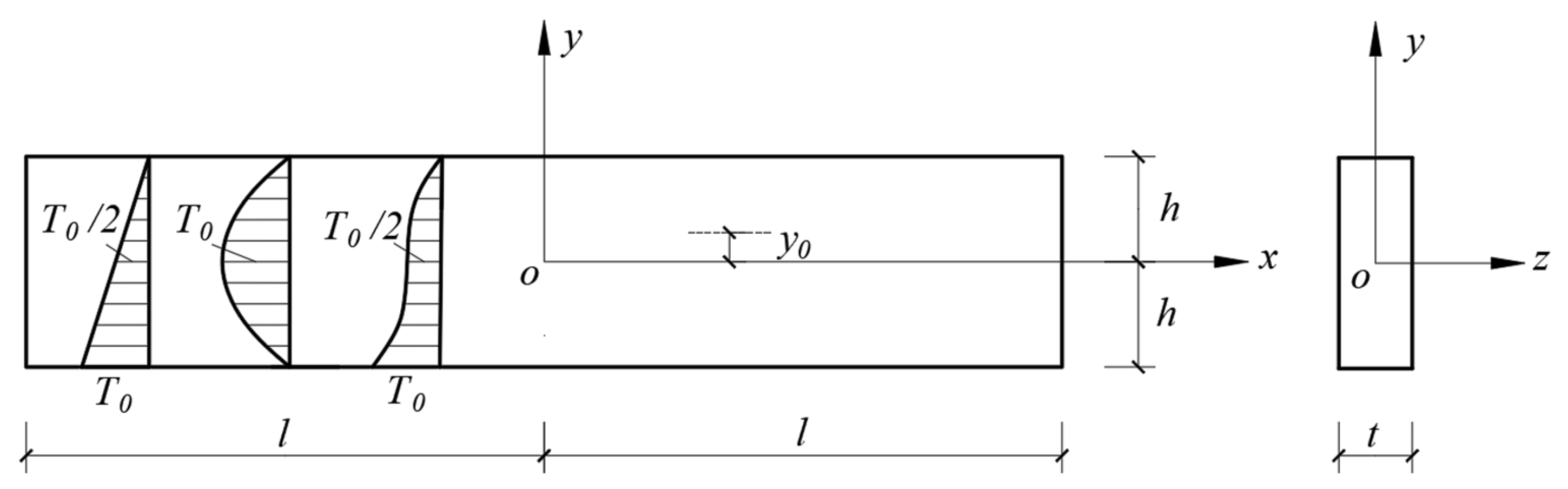
2.1. Problem

Let us consider the thermal stress in a bimodular bar with the length 2l, the height 2h and the thickness t under the specific temperature rise modes, as shown in Figure 2, in which the origin o of the coordinate system (o-xyz) is located at the centroid of the cross section of the bar. For beams and plates, it is generally assumed that temperature rise modes T vary only with the thickness direction [1,20], and thus, in this study, T = T(y). For the convenience of mathematical treatment, the T(y) is considered as a simple function in the form. Thus, the following three temperature rise modes are assumed:
Case   1 : T ( y ) = T 0 2 ( 1 y h ) ;
Case   2 : T ( y ) = T 0 ( 1 y 2 h 2 ) ;
Case   3 : T ( y ) = T 0 2 ( 1 y 3 h 3 ) ,
which corresponds to the linear, parabolic and cubic rise, respectively. Note that the linear rise satisfies the heat conduction equation while the parabolic and cubic rises cannot and they are unrealistic. However, here we only present a theoretical study on a bimodular bar under different temperature rise modes although the parabolic and cubic rises are imaginary. Among the three cases, the highest rise T0 is uniform and constant, in which for Case 2, T0 takes place at the middle of height direction of the bar while for Cases 1 and 3, T0 both take place at the bottom of the bar, as shown in Figure 2.
Note that unlike the common analysis, the materials made of the bar in this study are considered as bimodular materials whose the tensile Young’s modulus E+ is different from the compressive one E. At the same time, for simplicity the Poisson ratio of the bimodular materials are considered the same, while the linear thermal expansion coefficient is considered different in tension and compression, that is, we have the singular μ and different α+ and α. Additionally, note that y0 in Figure 2 stands for the location of the neutral axis when the bar is under pure bending, which may be determined thereafter.

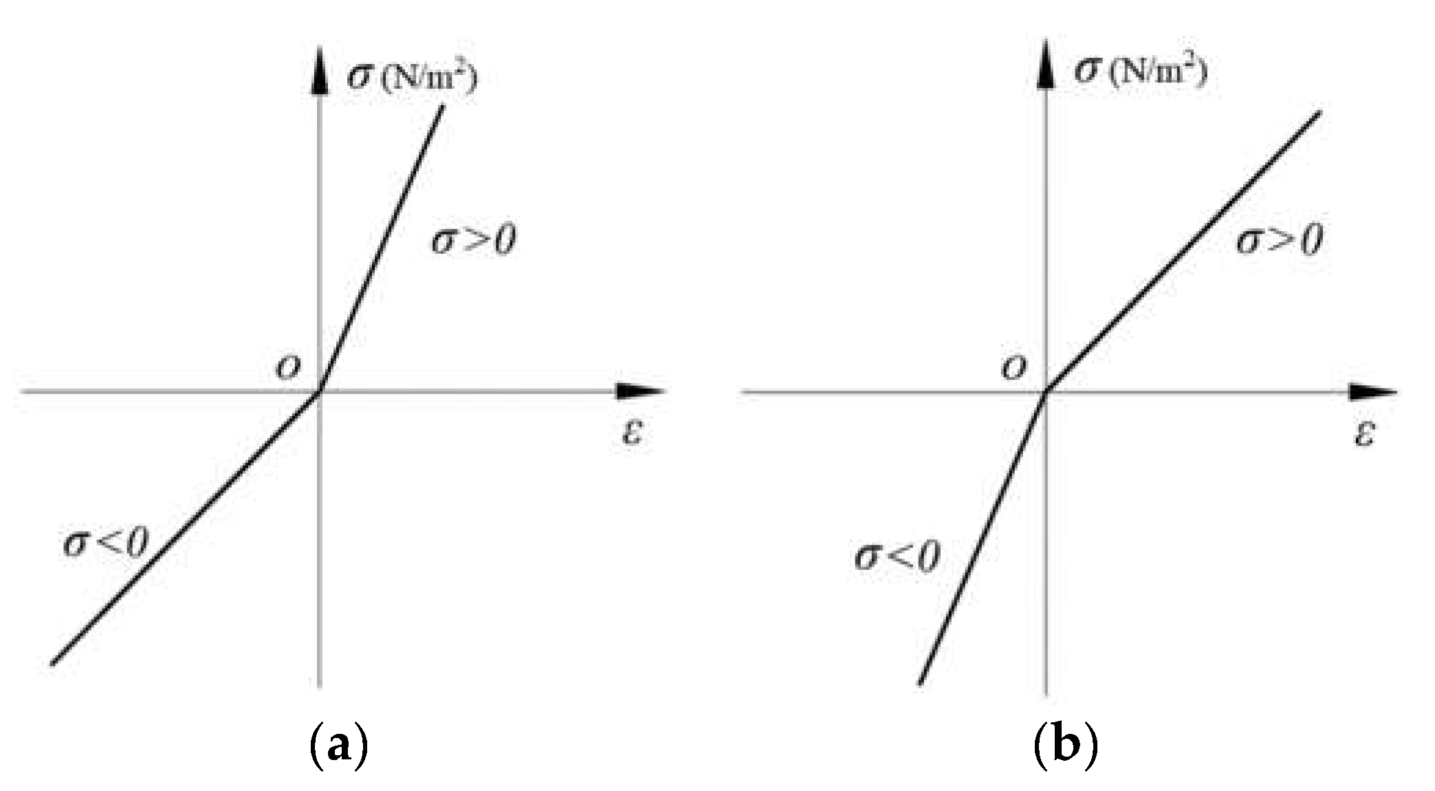
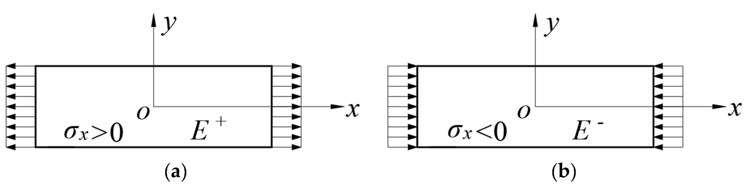
2.2. Bimodular Effect

According to the theory of elasticity of different moduli founded by Ambartsumyan [10], the so-called tensile or compressive modulus of a certain point is defined as whether the principal stress at this point is positive or negative, with the positive corresponding to tensile and the negative corresponding to compressive. In other words, if the point is in tension along the principal direction, the modulus here is taken as E+, while in compression along the principal direction, the modulus should be changed to E. Obviously, in a three-dimensional space problem, the constitutive law of bimodular materials which is established on the criterion of positive-negative signs of principal stress is somewhat complicated. However, in a one-dimensional stress state of tension or compression, or in a pure bending problem, it is easy for us to describe the constitutive law. More specifically, as shown in Figure 3, when a prismatic bar is subjected to pure axial tension, it is in the stress state of uniaxial tension, and we should take E+ here; on the contrary, when the bar is subjected to pure axial compression, E should be taken since it is in the stress state of uniaxial compression.
Compared to uniaxial tension or compression, the bimodular problem of bars under pure bending is somewhat complicated, this may be one of the problems that entered scholars’ vision earlier. As shown in Figure 4, a rectangular section bar with a height of 2h and thickness t, is subjected to the bending moment M at two ends and we isolate it apart from the whole bar as our studied object. Obviously, the bar will deflect downward to resist the external bending moment, thus, resulting in tension in the lower part of the bar and compression in the upper part. For convenience, we establish the x axis of the coordinate system (xoy) on the unknown neutral axis which may be determined thereafter. The height of the tensile part of the bar is h1 and the corresponding modulus is taken as E+; at the same time, the compressive height and the modulus is h2 and E, respectively, as shown in Figure 4.
In the light of the assumption of the plane section, the curvature ρ of the neutral axis may be expressed as:
1 ρ = d θ d x ,
in which, dx and dθ denote the length and rotation angle of a segment on the neutral axis, respectively, as shown in Figure 4. According to the basic definition of strain, for a certain segment with distance y from the neutral axis, its relative elongation, εx, is equal to:
ε x = y d θ d x = y ρ .
where a minus symbol is added to agree with the conventional “+” for tension and “−“ for compression, since here the positive direction of the y axis is upward while the bending moment M makes the beam convex downward, see Figure 4. Thus, we have the tensile normal stress and compressive normal one as follows:
{ σ x + = E + y ρ h 1 y 0 σ x = E y ρ 0 y h 2 .
Due to the pure bending, the equation of equilibrium gives:
h 1 0 σ x + t d y + 0 h 2 σ x t d y = 0
and
h 1 0 σ x + y t d y + 0 h 2 σ x y t d y = M ,
where the minus symbol before the bending moment M is based on the consideration that the convex direction produced by the bending moment is inconsistent with the positive direction of the y axis. Combining Equations (3) and (4) yields:
E + h 1 2 = E h 2 2 .
After considering h1 + h2 = 2h, we have
h 1 = E E + + E 2 h , h 2 = E + E + + E 2 h ,
which determines the location of the unknown neutral axis. Similarly, combining Equations (3) and (5) yields:
1 ρ ( E + t h 1 3 3 + E t h 2 3 3 ) = M .
If we define the bending stiffness D of the bimodular beam as:
D = t 3 ( E + h 1 3 + E h 2 3 ) ,
Equation (8) will return to our familiar form:
1 ρ = M D .
Substituting Equation (10) into Equation (3) gives the tensile and compressive stress as follows:
{ σ x + = M D / E + y = M I + y , h 1 y 0 σ x = M D / E y = M I y , 0 y h 2 ,
in which, I+ and I denote the tensile and compressive moment of inertia, respectively, and they are:
I + = t 3 ( h 1 3 + E E + h 2 3 ) , I = t 3 ( E + E h 1 3 + h 2 3 ) .
Besides, from Figure 2 and Figure 4, it is easy to see that h + y0 = h1 or hy0 = h2. Combining Equation (7), we have the coordinate location of the neutral axis:
y 0 = E E + E + E + h .
The above expressions may be reduced to the classical forms when E+ = E = E and h1 + h2 = h; and next we will use these results for the analysis of thermal stress of bimodular problems, in which the axial tension or compression and pure bending are included.

3. Two Basic Methods

3.1. Strain Suppression Method

Let us consider a metal bar with uniform thickness in a thermal environment, in which the temperature T is a function of y and is independent of x and z, as shown in Figure 2. The longitudinal thermal expansion αT will be entirely suppressed by applying to the whole bar the longitudinal stress [1]:
σ x = α E T ( = α E T ) ,
which is compressive when T is positive. In fact, this stress is always compressive under the three temperature rise modes shown in Figure 2, thus, each point of the bar is in the state of compression. If here we introduce the different moduli in tension and compression, the elastic modulus E in Equation (14) may be changed as E, and also the thermal expansion coefficient α is changed as α accordingly while E = E, as shown in Equation (14). Besides, we note that the application of the above stress (14) will not produce stress in the lateral directions since the bar is free to expand laterally.
To maintain the stress (14) throughout the bar, it will be necessary to distribute compressive forces of the magnitude (14) at the two ends of the bar only. These compressive forces will completely suppress any expansion of the bar along the x direction due to the temperature rise T. In order to obtain the thermal stress in the bar, which is free from external forces, we have to superpose on the stress (14), the stresses produced in the bar by tensile forces of intensity αTE distributed at the ends. These forces have the result h + h α E T ( y ) d y , and at a sufficient distance from the ends, they will produce approximately uniformly distributed tensile stress of the magnitude 1 2 h h + h α + E + T ( y ) d y , in which the elastic modulus E has been changed to E+ and also the thermal expansion coefficient α is changed as α + accordingly since it is always tensile stress. Therefore, the thermal stress in the bar with free ends, at a sufficient distance from the ends, will be:
σ x = α E T ( y ) + 1 2 h h + h α + E + T ( y ) d y .
If the temperature T is symmetrical with respect to the x axis, for example, in Case 2 in Figure 2, Equation (15) will be the final result of the thermal stress, even the introduction of the bimodular effect does not change this characteristic. For Cases 1 and 3 in Figure 2, however, the temperature T is not symmetrical with respect to the x axis, we must superpose on the compressive stress (14) a uniform tension, determined as before, and bending stress determined from the condition that the moment of the forces distributed over a cross section must be zero, y I h + h α E T ( y ) y t d y , in which I is the moment of inertia of the cross section. If the bimodular effect is introduced here, the bending stress may be calculated in the form of piecewise integral, y I + h y 0 α + E + T ( y ) y t d y + y I y 0 + h α E T ( y ) y t d y , in which y0 is the location of the neutral axis and its expression is shown in Equation (13), and I+ and I denote the tensile and compressive moment of inertia, respectively, and their expressions are shown in Equation (12). Note that here we assume the tension takes place at the lower part of the bar and the compression at the upper part, that is, for the cross section of the bar, the lower in tension and the upper in compression. Or alternatively, it may be the lower in compression and the upper in tension. Which situation we take will depend on the real problem. More specially, if the linear and cubic temperature rises take place, as shown in Figure 2, the bending mode should be the lower in tension and the upper in compression to agree with the basic idea of strain suppression. Eventually, the total thermal stress is:
σ x = α E T ( y ) + 1 2 h h + h α + E + T ( y ) d y + y I + h y 0 α + E + T ( y ) y t d y + y I y 0 + h α E T ( y ) y t d y .

3.2. Thermoelasticity Method

Letting εx, εy and γxy to be the strain components of a plane stress problem and σx, σy and τxy are the corresponding stress components, the physical equation of thermoelasticity theory may be directly given as follows [1]:
{ ε x = 1 E + / ( σ x μ σ y ) + α + / T ε y = 1 E + / ( σ y μ σ x ) + α + / T γ x y = 2 ( 1 + μ ) E + / τ x y ,
in which, the tensile-compressive Young’s modulus is denoted by E+/−, E+ corresponding to the tensile modulus and E to the compressive one. Similarly, α+/− has the same meaning as E+/−. In our study, there is no way to specify, from the very beginning, the stress state of any point, tensile or compressive. Therefore, we have to use this form E+/− and α+/− to express the physical equation for the time being.
Via geometrical equation and equation of equilibrium, we may have the Lamé equation expressed in terms of the displacement u and v and the temperature variation T:
{ 2 u x 2 + 1 μ 2 2 u y 2 + 1 + μ 2 2 v x y ( 1 + μ ) α + / T x = 0 2 v y 2 + 1 μ 2 2 v x 2 + 1 + μ 2 2 u x y ( 1 + μ ) α + / T y = 0 ,
and the stress boundary condition:
{ l ( u x + μ v y ) s + m 1 μ 2 ( u y + v x ) s = l ( 1 + μ ) α + / T m ( v y + μ u x ) s + l 1 μ 2 ( v x + u y ) s = m ( 1 + μ ) α + / T ,
in which, l and m are direction cosines. Similar to [25], from Equations (18) and (19) it is also found that based on the classical Duhamel theorem concerning body force analogy, the thermal plane stress problem may be transformed into a classical plane stress problem.
For obtaining the special solution of Equation (18), we introduce a potential function of displacement, ψ(x,y), and at the same time the special solution of displacement may be taken as:
u = ψ x , v = ψ y .
Regarding the u’ and v’ as u and v, and substituting them into Equation (18), we have:
{ x 2 ψ = ( 1 + μ ) α + / T x y 2 ψ = ( 1 + μ ) α + / T y .
Note that μ and α+/− are both constants, indicating that if the function ψ(x,y) can satisfy the following differential equation:
2 ψ = ( 1 + μ ) α + / T ,
the ψ(x,y) can satisfy Equation (21), thus also satisfying Equation (18). Finally, the u’ and v’ in Equation (20) may be selected as a special solution. Substituting Equations (20) and (22) into Equation (18), we obtain the stress component corresponding to the special solution:
σ x = E + / 1 + μ 2 ψ y 2 ,   σ y = E + / 1 + μ 2 ψ x 2 ,   τ x y = E + / 1 + μ 2 ψ x y .
On the other hand, the supplement solution of displacement, u’’ and v’’, needs to satisfy the homogeneous equation of Equation (18), that is:
{ 2 u x 2 + 1 μ 2 2 u y 2 + 1 + μ 2 2 v x y = 0 2 v y 2 + 1 μ 2 2 v x 2 + 1 + μ 2 2 u x y = 0 .
Via Equation (17) and also T = 0, we have the stress components corresponding to the supplement solution:
{ σ x = E + / 1 μ 2 ( u x + μ v y ) σ y = E + / 1 μ 2 ( v y + μ u x ) τ x y = E + / 2 ( 1 + μ ) ( v x + u y ) .
Eventually, the total stress components are:
σ x = σ x + σ x , σ y = σ y + σ y , τ x y = τ x y + τ x y   ,
which need to satisfy stress boundary conditions. In addition, we introduce a stress function, ϕ(x,y), to express the stress components corresponding to the supplement solution, that is [1]:
  σ x = 2 φ x 2 , σ y = 2 φ y 2 , τ x y = 2 φ x y .

4. One-Dimensional Solution Based on Strain Suppression Method

4.1. Case 1: T ( y ) = T 0 2 ( 1 y h )

By using the strain suppression method and also considering the different moduli in tension and compression, we have the thermal stress expression in the bimodular bar, this is, Equation (16). Substituting the T(y), I+ and I from Equation (12) into Equation (16) and integrating, we obtain:
σ x = T 0 2 { α E ( 1 y h ) + α + E + + 3 y E + h 1 3 + E h 2 3 [ α + ( E + ) 2 ( y 0 2 2 y 0 3 3 h 5 h 2 6 ) α ( E ) 2 ( y 0 2 2 y 0 3 3 h h 2 6 ) ] } .
Alternatively, for the computation of the bending stress, if we neglect the difference of I+ and I, and also regard I+ = I = I = 2th3/3, a simpler expression may be obtained as:
σ x = T 0 2 { α E ( 1 y h ) + α + E + + 3 2 y h [ α + E + ( 1 2 y 0 2 h 2 1 3 y 0 3 h 3 5 6 ) α E ( 1 2 y 0 2 h 2 1 3 y 0 3 h 3 1 6 ) ] } .
Note that without the bimodular effect, E+ = E = E, α+ = α = α, we may have h1 = h2 = h and y0 = 0, thus Equations (28) and (29) both give σx = 0, which verifies the familiar conclusion that under the linear temperature rise mode, there exists no thermal stress in the bar without bimodular effect.

4.2. Case 2: T ( y ) = T 0 ( 1 y 2 h 2 )

In this case, the temperature T(y) is symmetrical with respect to the x axis, the bending moment does not occur, even if the bimodular effect is considered, thus, we have the thermal stress expression that is the same as Equation (15). Substituting the T(y) into Equation (15) and integrating, we obtain:
σ x = T 0 [ α E ( 1 y 2 h 2 ) + 2 3 α + E + ] .
When E+ = E = E, α+ = α =α, we have:
σ x = α E T 0 ( y 2 h 2 1 3 ) ,
which agrees with the common expression.

4.3. Case 3: T ( y ) = T 0 2 ( 1 y 3 h 3 )

Similar to Case 1, we have the thermal stress expression in this case that is the same as Equation (16), in which the bending stress exists since T(y) is not symmetrical with respect to the x axis. Substituting the T(y), I+ and I from Equation (12) into Equation (16) and integrating, we obtain:
σ x = T 0 2 { α E ( 1 y 3 h 3 ) + α + E + + 3 y E + h 1 3 + E h 2 3 [ α + ( E + ) 2 ( y 0 2 2 y 0 5 5 h 3 7 h 2 10 ) α ( E ) 2 ( y 0 2 2 y 0 5 5 h 3 3 h 2 10 ) ] } .
Similar to Case 1, the computation of the bending stress may be further simplified by taking I+ = I = I =2th3/3, another simpler expression may be obtained as:
σ x = T 0 2 { α E ( 1 y 3 h 3 ) + α + E + + 3 2 y h [ α + E + ( 1 2 y 0 2 h 2 1 5 y 0 5 h 5 7 10 ) α E ( 1 2 y 0 2 h 2 1 5 y 0 5 h 5 3 10 ) ] } .
When E+ = E = E, α+ = α = α, we have h1 = h2 =h and y0 = 0, thus Equations (32) and (33) return to:
σ x = α E T 0 2 ( y 3 h 3 3 5 y h ) ,
which is the same as that of the singular modulus problem and also verifies the correctness of the derivation from the side.

5. Two-Dimensional Thermoelasticity Solution

5.1. Case 1: T ( y ) = T 0 2 ( 1 y h )

Under the temperature variation T(y), Equation (22) which the potential function of displacement ψ should satisfy now becomes:
2 ψ = ( 1 + μ ) α + / T 0 2 ( 1 y h ) .
Obviously, if we take:
ψ = A y 2 + B y 3 ,
it may satisfy Equation (35), in which A and B are two undetermined constants. Substituting Equation (36) into Equation (35) and comparing the coefficients at two sides, we have:
A = ( 1 + μ ) α + / T 0 4 , B = ( 1 + μ ) α + / T 0 12 h .
Thus, the potential function of displacement is:
ψ = ( 1 + μ ) α + / T 0 4 ( y 2 y 3 3 h ) .
Via Equation (23), the stress component corresponding to the special solution of displacement gives:
σ x = T 0 2 α + / E + / ( y h 1 ) , σ y = 0 ,   τ x y = 0 .
Note that in the final solution, the modulus of elasticity and the thermal expansion coefficient in σx’ should be rectified as E and α, respectively, since this term always corresponds to the compressive stress. However, this term is still given in the form of tension or compression for the time being since, in the next integration, the plus and negative symbol will be changed as the state in tension and compression.
It is found that from Equation (39) the distribution of this stress on the left and right sides of the bar is also linear and compressive. For satisfying the boundary conditions, a surface force, equal in magnitude and opposite in direction, may be exerted on the left and right sides of the bar, thus, the stress caused by this surface force may serve as a supplement solution, this is, σx’’, σy’’ and τy’’, to be superimposed on the special solution presented in Equation (39). If the two plane dimensions of the bar, 2l and 2h, are in the same order of magnitude, it is hard to obtain the analytical expression of this supplement solution, in this case, numerical methods have to be resorted to. However, if l >> h, as shown in Figure 2, the left and right ends of the bar become the second boundary, thus, making the application of the de Saint-Venant Principle possible. According to the principle of statics equivalence, the uneven surface force on the left and right ends of the bar should be counteracted by a uniform tension and a bending moment. For this purpose, the following stress function is adopted:
φ = c y 2 + e y 3 ,
in which c and e are two undetermined constants, the term cy2 corresponds to the uniform tension while the term ey3 to the pure bending. The corresponding stress components are:
σ x = 2 c + 6 e y , σ y = τ x y = 0 .
Adding them to the stress in Equation (39), we have the total stress components:
{ σ x = σ x + σ x = T 0 2 α + / E + / ( y h 1 ) + 2 c + 6 e y σ y = σ y + σ y = 0 τ x y = τ x y + τ x y = 0 ,
which should satisfy the following boundary conditions:
( σ x ) x = ± l = 0 , ( τ x y ) x = ± l = 0 , ( σ y ) y = ± h = 0 , ( τ x y ) y = ± h = 0 ,
in which, the last three conditions are satisfied naturally while the first one may be approximately satisfied by using de Saint-Venant Principle. Thus, we have:
h + h ( σ x ) x = ± l d y = 0
and
h + h ( σ x ) x = ± l y t d y = 0 .
Substituting the expression of σx in Equation (42) into Equation (43), we have:
h + h [ T 0 2 α + / E + / ( y h 1 ) + 2 c + 6 e y ] d y = 0 ,
which gives 2c = T0α+/−E+/−/2. As indicated earlier, the term 2c corresponds to the uniform tension, this term should be changed to:
2 c = T 0 2 α + E + .
Similarly, substituting the expression of σx in Equation (42) into Equation (45), we have:
h + h [ T 0 2 α + / E + / ( y h 1 ) + T 0 2 α + E + + 6 e y ] y t d y = 0 .
Note that the term T0α+E+/2 does not contribute to bending moment, thus, it may be deleted in Equation (48) first. Generally, the bending moment is always accompanied by tension and compression; therefore, the computation for the bending moment should be carried out in the tensile area and in compressive area. According to the real temperature rise in Case 1, the highest temperature takes place at the bottom of the bar. It may be speculated that the lower part of the bar is in tension and the upper part of the bar in compression, thus the integration should be modified as:
h y 0 [ T 0 2 α + E + ( y h 1 ) + 6 e y ] y t d y + y 0 + h [ T 0 2 α E ( y h 1 ) + 6 e y ] y t d y = 0 .
The unknown constant e may be determined as:
e = T 0 8 h [ α + E + ( 1 2 y 0 2 h 2 1 3 y 0 3 h 3 5 6 ) α E ( 1 2 y 0 2 h 2 1 3 y 0 3 h 3 1 6 ) ] .
Thus, the final stress solution is:
σ x = T 0 2 { α E ( 1 y h ) + α + E + + 3 2 y h [ α + E + ( 1 2 y 0 2 h 2 1 3 y 0 3 h 3 5 6 ) α E ( 1 2 y 0 2 h 2 1 3 y 0 3 h 3 1 6 ) ] } , σ y = τ x y = 0 .
in which, the modulus of elasticity and thermal expansion coefficient of the first term in σx has been changed as E and α, as indicated earlier. After comparing Equation (51) with Equations (28) and (29), it is found that Equation (51) is the same as Equation (29), having a slight difference with Equation (28) that is caused mainly by the different moments of inertia.

5.2. Case 2: T ( y ) = T 0 ( 1 y 2 h 2 )

Under the temperature variation T(y), Equation (22) now becomes:
2 ψ = ( 1 + μ ) α + / T 0 ( 1 y 2 h 2 ) .
Obviously,
ψ = A y 2 + B y 4
may satisfy Equation (52). Substituting Equation (53) into Equation (52) and comparing the coefficients at two sides, we have:
A = ( 1 + μ ) α + / T 0 2 , B = ( 1 + μ ) α + / T 0 12 h 2 .
Thus, the potential function of displacement is:
ψ = ( 1 + μ ) α + / T 0 ( y 2 2 y 4 12 h 2 ) .
Via Equation (23), the stress component corresponding to the special solution of displacement gives:
σ x = T 0 α + / E + / ( y 2 h 2 1 ) ,   σ y = 0 ,   τ x y = 0 .
Due to the fact that under the temperature rise, there exists no bending moment, we take the following stress function:
φ = c y 2 ,
which corresponds to the uniform tension on the left and right ends of the bar. The corresponding stress components are:
σ x = 2 c , σ y = τ x y = 0 .
Adding them to the stress in Equation (56), we have the total stress components:
{ σ x = σ x + σ x = T 0 α + / E + / ( y 2 h 2 1 ) + 2 c σ y = σ y + σ y = 0 τ x y = τ x y + τ x y = 0 .
They should satisfy the boundary conditions which are the same as Equation (43). Similarly, the last three conditions are satisfied naturally while the first one may be approximately satisfied by using the de Saint-Venant Principle. Thus, we have Equations (44) and (45) again, in which Equation (45) has been satisfied naturally. Substituting the expression of σx in Equation (59) into Equation (44), we have:
h + h [ T 0 α + / E + / ( y 2 h 2 1 ) + 2 c ] d y = 0 ,
which gives 2c = 2T0α+/−E+/−/3. As indicated earlier, the term 2c corresponds to the uniform tension, thus this term should be rectified as:
2 c = 2 3 T 0 α + E + .
Thus, the final stress solution is:
σ x = T 0 [ α E ( 1 y 2 h 2 ) + 2 3 α + E + ] , σ y = τ x y = 0 ,
in which, the first term has been modified as the compressive quantities. After comparing it with Equation (30), it is found that they are the same.

5.3. Case 3: T ( y ) = T 0 2 ( 1 y 3 h 3 )

Similar to Case 1, Equation (22) now becomes:
2 ψ = ( 1 + μ ) α + / T 0 2 ( 1 y 3 h 3 ) .
Obviously,
ψ = A y 2 + B y 5
may satisfy Equation (63). Substituting Equation (64) into Equation (63) and comparing the coefficients at two sides, we have:
A = ( 1 + μ ) α + / T 0 4 , B = ( 1 + μ ) α + / T 0 40 h 3 .
Thus, the potential function of displacement is:
ψ = ( 1 + μ ) α + / T 0 2 ( y 2 2 y 5 20 h 3 ) .
Via Equation (23), the stress component corresponding to the special solution of displacement gives:
σ x = α T 0 2 α + / E + / ( y 3 h 3 1 ) ,   σ y = 0 ,   τ x y = 0 .
The following stress function is adopted:
φ = c y 2 + e y 3 ,
in which, cy2 corresponds to the uniform tension while ey3 to the pure bending. The corresponding stress components are:
σ x = 2 c + 6 e y , σ y = τ x y = 0 .
Adding them to the stress in Equation (67), we have the total stress components:
{ σ x = σ x + σ x = T 0 2 α + / E + / ( y 3 h 3 1 ) + 2 c + 6 e y σ y = σ y + σ y = 0 τ x y = τ x y + τ x y = 0 .
They should satisfy the boundary conditions of the bar with four sides free, as shown in Equation (43). Similarly, the last three conditions are satisfied naturally while the first one may be approximately satisfied by using the de Saint-Venant Principle. Thus, we have Equations (44) and (45) once again. Substituting the expression of σx into Equation (44), we have:
h + h [ T 0 2 α + / E + / ( y 3 h 3 1 ) + 2 c + 6 e y ] d y = 0 ,
which gives 2c = α+/−T0E+/−/2. As indicated earlier, the term 2c corresponds to the uniform tension, this term should be changed to:
2 c = T 0 2 α + E + .
Substituting the expression of σx into Equation (45), we have:
h + h [ T 0 2 α + / E + / ( y 3 h 3 1 ) + T 0 2 α + E + + 6 e y ] y t d y = 0 .
Similar to Case 1, the integration may be changed as:
h y 0 [ T 0 2 α + E + ( y 3 h 3 1 ) + 6 e y ] y t d y + y 0 + h [ T 0 2 α E ( y 3 h 3 1 ) + 6 e y ] y t d y = 0 ,
leading to:
e = T 0 8 h [ α + E + ( 1 2 y 0 2 h 2 1 5 y 0 5 h 5 7 10 ) α E ( 1 2 y 0 2 h 2 1 5 y 0 3 h 3 3 10 ) ] .
Thus, the final stress solution is:
σ x = T 0 2 { α E ( 1 y 3 h 3 ) + α + E + + 3 2 y h [ α + E + ( 1 2 y 0 2 h 2 1 5 y 0 5 h 5 7 10 ) α E ( 1 2 y 0 2 h 2 1 5 y 0 3 h 3 3 10 ) ] } , σ y = τ x y = 0
After comparing Equation (76) with Equations (32) and (33), it is found that Equation (76) is the same as Equation (33), also having a slight difference with Equation (32) that is caused mainly by the different moments of inertia.

6. Results and Discussions

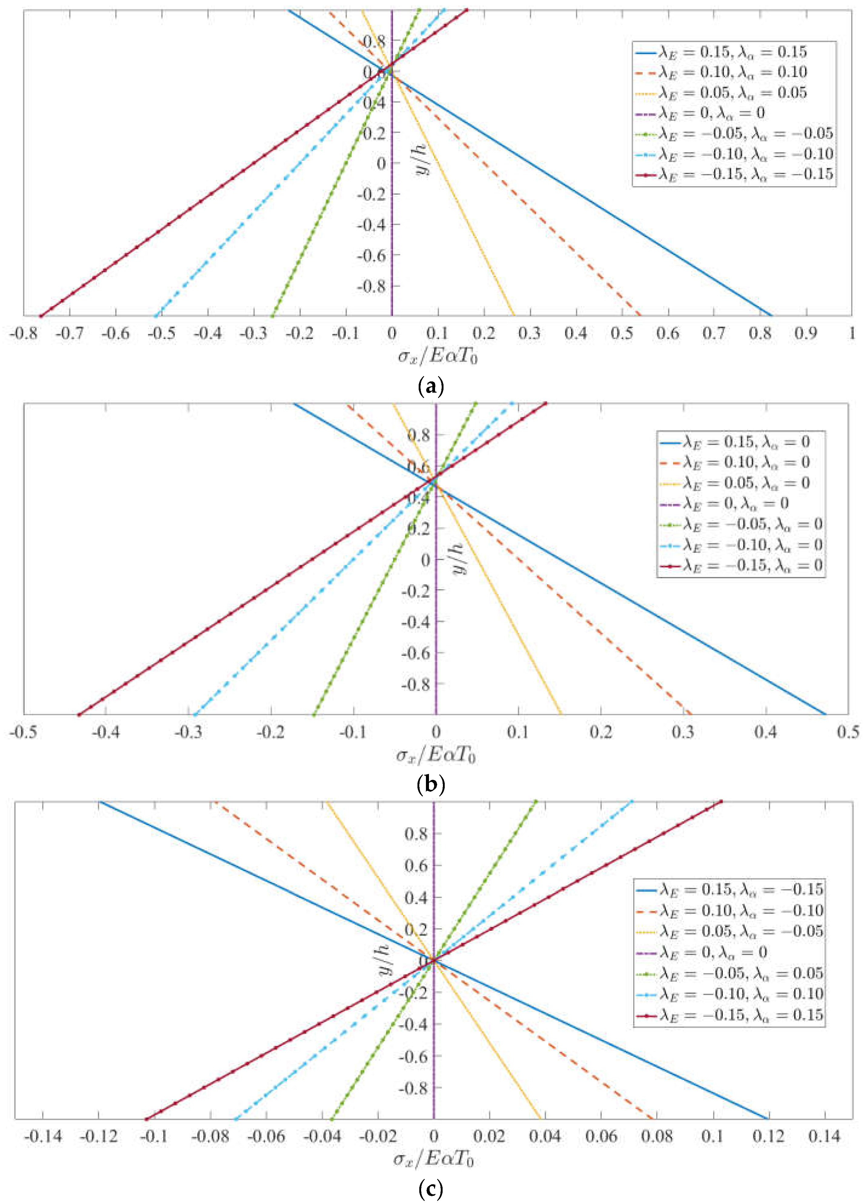
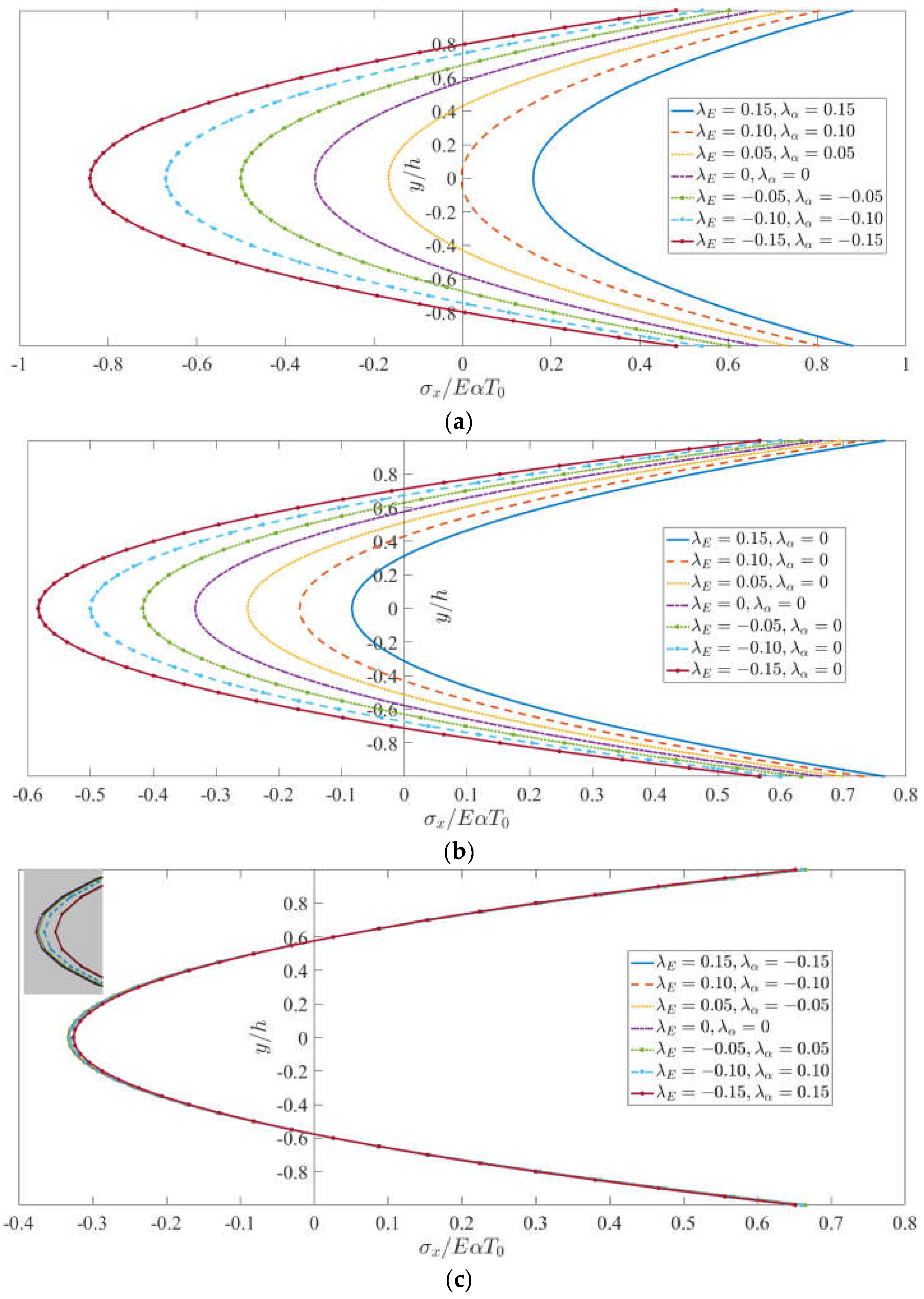
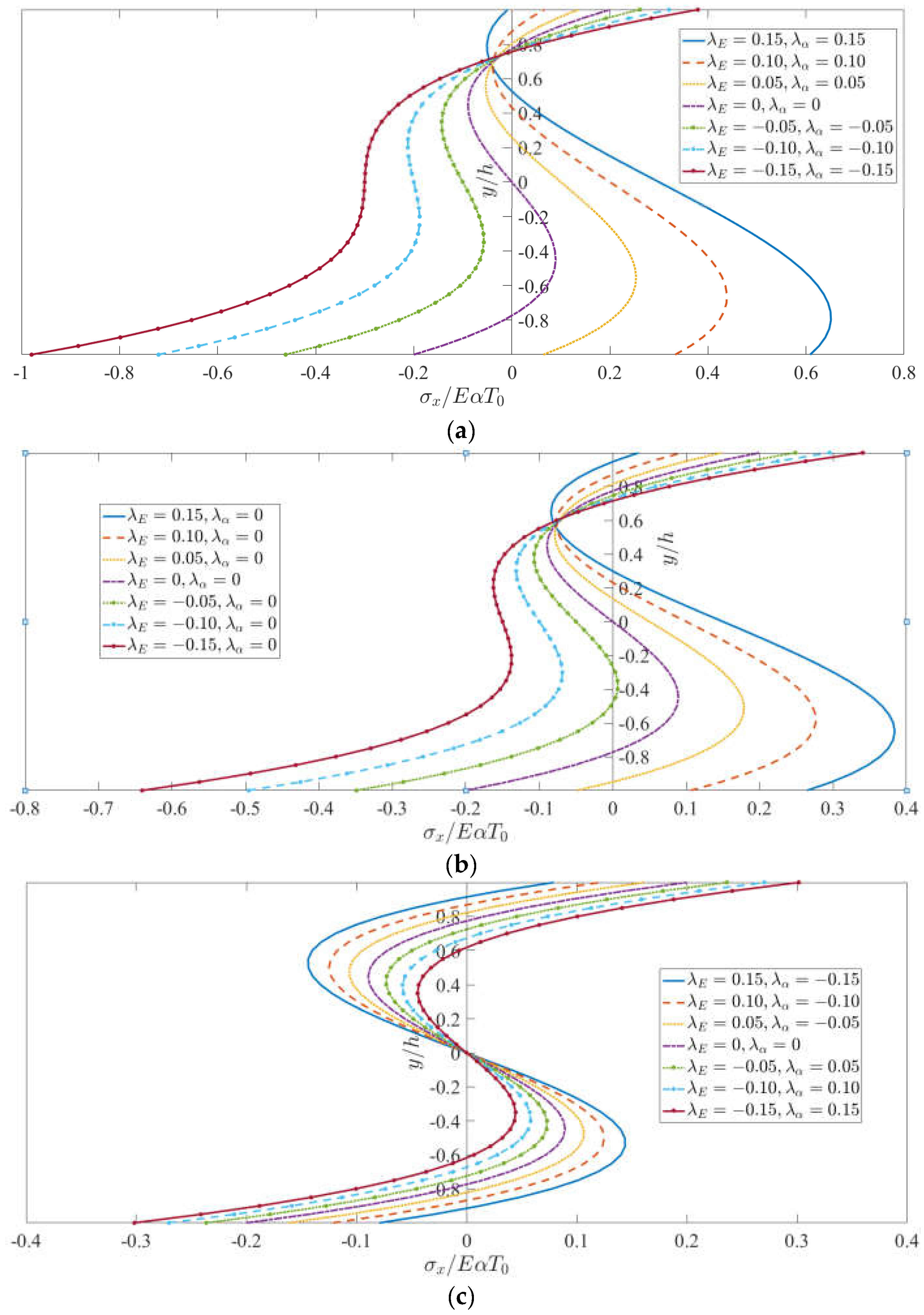
6.1. Bimodular Effect on Thermal Stress

In order to investigate the bimodular effect on thermal stress, let us introduce the following relations [31]:
E = E + + E 2 , λ E = E + E E + + E , E + = ( 1 + λ E ) E , E = ( 1 λ E ) E α = α + + α 2 , λ α = α + α α + + α , α + = ( 1 + λ α ) α , α = ( 1 λ α ) α
In which the relationship among α, α+, α and λα is introduced by simulating the relationship among E, E+, E and λE. In Equation (77), E and α is the average modulus and average heat expansion coefficient, respectively, and λE and λα are two important ratios of the difference to the sum, and their values are relatively small by definition, and also indicating that when λE > 0, E+ > E; λE < 0, E+ < E and λα also has the same regulation, that is, λα > 0, α+ > α; λα < 0, α+ < α. Substituting the relation (77) into the thermal stress expressions in three cases, that is, Equations (28), (30) and (32), we have, for Case 1,
σ x = E α T 0 { ( 1 λ E ) ( 1 λ α ) 2 ( 1 y h ) + ( 1 + λ E ) ( 1 + λ α ) 2 + 3 y ( 1 + λ E ) h 1 3 + ( 1 λ E ) h 2 3 × [ ( 1 + λ E ) 2 ( 1 + λ α ) 2 ( y 0 2 2 y 0 3 3 h 5 h 2 6 ) ( 1 λ E ) 2 ( 1 λ α ) 2 ( y 0 2 2 y 0 3 3 h h 2 6 ) ] } ,
for Case 2,
σ x = E α T 0 [ ( 1 λ E ) ( 1 λ α ) ( 1 y 2 h 2 ) + 2 3 ( 1 + λ E ) ( 1 + λ α ) ] ,
and for Case 3,
σ x = E α T 0 { ( 1 λ E ) ( 1 λ α ) 2 ( 1 y 3 h 3 ) + ( 1 + λ E ) ( 1 + λ α ) 2 + 3 y ( 1 + λ E ) h 1 3 + ( 1 λ E ) h 2 3 × [ ( 1 + λ E ) 2 ( 1 + λ α ) 2 ( y 0 2 2 y 0 5 5 h 3 7 h 2 10 ) ( 1 λ E ) 2 ( 1 λ α ) 2 ( y 0 2 2 y 0 5 5 h 3 3 h 2 10 ) ] } ,
in which, h1 and h2, as well as y0, are expressed in terms of λE, respectively:
h 1 = 1 λ E 1 + λ E + 1 λ E 2 h , h 2 = 1 + λ E 1 + λ E + 1 λ E 2 h ,
and
y 0 = 1 λ E 2 1 λ E h .
For the common metals and their oxides, the difference of tensile modulus and compressive one is generally small but there does exist such a difference that may influence the thermal stress. The data in Table 1 are taken from the classical monograph which was written by Ambartsumyan, in which the λE values are computed based on the relation from Equation (77), λE = (E+E)/(E+ + E). It is easy to see that the abstract value of λE is relatively small, ranging from 0 to 0.15. Therefore, in our study, the parameter λE is taken as seven different values and they are 0.15, 0.10, 0.05, 0, −0.05, −0.10 and −0.15, in which the former three values correspond to the case E+ > E, the latter three values correspond to E+ < E and λE = 0 corresponds to E+ = E.
In the current studies, no reports of the different moduli effects on the thermal expansion coefficient of metals have been found. However, this is the main purpose of this theoretical study. For predicting theoretically the variation trend of linear expansion coefficients with the bimodular effect, we take the following three groups’ values for comparisons, that is, when λE is taken as 0.15, 0.10, 0.05, 0, −0.05, −0.10 and −0.15 in turn, in Group 1, λα is also taken as 0.15, 0.10, 0.05, 0, −0.05, −0.10 and −0.15 in turn, that is, the variation trend of λα is consistent to λE, both changing from 0.15 to −0.15; in Group 2, λE keeps the original change trend, and there is no any change between α+ and α, that is, λα = 0 and in Group 3, λα is taken as −0.15, −0.10, −0.05, 0, 0.05, 0.10 and 0.15 in turn, that is, the variation trend of λα is contrary to that of λE. Figure 5a–c plot the thermal stress for Case 1 under different λE and λα values, Figure 6a–c is for Case 2 and Figure 7a–c is for Case 3, in which the horizontal axis stands for the dimensionless thermal stress σx/EαT0 and their expressions are shown in Equations (78)–(80), and the vertical axis stands for the height direction of the cross section, also given in dimensional form y/h.
From Figure 5a–c, Figure 6a–c and Figure 7a–c, we may have the following results and corresponding discussions.
(i)
Basic curve shapes:
First, Figure 5a–c, Figure 6a–c and Figure 7a–c show that all curves follow the variation trend shown in Equations (78)–(80), presenting the linear, parabolic and cubic relation, respectively.
(ii)
Neutral axes and stress distributions:
Note, that in this study there are two different notions concerning the neutral axis, one is the bending neutral axis due to pure bending that we analyzed in Section 2.2 and the location for the unknown neutral axis may be determined as long as the magnitude of tensile and compression modulus of elasticity is known, as shown in Equation (7); another notion is the so-called final neutral axis with thermal effect, due to the combination of the compressive axial force, and tensile axial force and the corresponding bending moment, as shown in Equation (16).
From Figure 5c it is seen that for Case 1, regardless of different λE values, there is only one position of the neutral axis, this means that for each λE value, there is one position of neutral axis corresponding to it. When λE = 0 (E+ = E), the curve is exactly on the axis y/h, indicating σx = 0 and there exists no neutral axis. When λE >0 (E+ > E), the cross section of the bar presents tension in the lower part and compression in the upper part, and when λE <0 (E+ < E) the cross section presents compression in the lower part and tension in the upper part. Figure 5c also shows that the linear temperature rise will produce unexpected thermal stress in a bimodular metal bar.
Figure 6c shows that there are two final neutral axes. It is easy to see from Figure 6c that there are, in fact, four curves but not seven curves since among the seven curves, the former three curves overlap completely with the latter three curves, the partially enlarged drawing show this phenomenon which may be easily validated from Equation (79).
Figure 7c shows that all curves present an S shape and have three intersects with the y/h axis, indicating that there are three final neutral axes. However, the introduction of different moduli changes the S shape to some extent. All curves pass the zero point, showing that there is no thermal stress in the center of the metal bar.
(iii)
Amplitudes of stress variation:
It is easy to see from Figure 5c, Figure 6c and Figure 7c that after the introduction of the bimodular effect, the amplitude of stress variation from the maximum tensile stress to the maximum compressive stress increased dramatically. Table 2 lists these amplitudes for Cases 1, 2 and 3 in the form of dimensionless quantity σx/EαT0, in which the largest amplitude change is Case 2 (parabolic temperature rise) and the smallest is Case 1 (linear temperature rise) and Case 3 (cubic temperature rise) is the middle. The amplitude of stress variation reflects the degree of stress variation in a limited region; this should be paid some attention to the design of components related to thermal stress, especially when the bimodular effect is introduced.

6.2. Discussions on the Compatibility

For the verification of the compatibility, first, we need to derive the compatibility equation expressed in terms of stress and temperature variation T. For this purpose, we substitute Equation (17) into the following compatibility equation expressed in terms of strain, that is:
2 ε x y 2 + 2 ε y x 2 = 2 γ x y x y .
Thus, we have:
2 y 2 ( σ x μ σ y E + / + α + / T ) + 2 x 2 ( σ y μ σ x E + / + α + / T ) = 2 x y [ 2 ( 1 + μ ) E + / τ x y ] .
On the other hand, letting the body force be zero, the equilibrium equation gives:
σ x x + τ x y y = 0 , σ y y + τ x y x = 0 .
Via Equation (85), we may obtain the relation 2 2 τ x y / x y = 2 σ x / x 2 2 σ y / y 2 which may be used for the simplification of Equation (84). Substituting it into Equation (84), the compatibility equation becomes:
2 ( σ x + σ y ) + E + / α + / 2 T = 0 .
in which, 2 stands for 2 / x 2 + 2 / y 2 . Now, substituting the thermal stress solutions (Equations (28), (30) and (32)) under three different temperature rise modes, into the compatibility Equation (86), respectively, also noting that σy = 0 and σx depends only on y, we have, for Case 1, due to T(y) = T0 (1–y/h)/2, Equation (86) is naturally satisfied after substituting Equation (28); for Case 2, T(y) = T0(1–y2/h2), substituting Equation (30) into Equation (86) gives:
2 T 0 α E 2 T 0 E + / α + / = 0 .
Obviously, if E+/−α+/− in the second term is appropriately selected, Equation (87) may be satisfied. More specially, if we let E+/−α+/− = Eα, Equation (87) is naturally satisfied, or alternatively if we select E+/−α+/− =E+α+, Equation (87) can also be satisfied by adding a restrictive condition, E+α+ = Eα, which is rational according to the next discussion on equilibrium. For Case 3, T(y) = T0(1–y3/h3)/2, substituting Equation (32) into Equation (86) gives:
3 T 0 α E y 3 T 0 E + / α + / y = 0 .
Similarly, Equation (88) is also satisfied according to the analysis above. Therefore, the stress solution satisfies the compatibility relation.

6.3. Discussions on the Equilibrium

First, the stress components must satisfy the equation of equilibrium. The verification of the equilibrium condition may begin with Equation (85). If we note σy = 0, τxy = 0 and σx depends only on y, it is easy to see that Equation (85) is easily satisfied. However, this seems to be inadequate since the stress solution in this study needs to satisfy the Lamé equation (Equation (18)).
In this study, because the obtainment for thermal stress solution is our main aim, and the displacement components are obtained as a secondary aspect, thus, it is difficult for us to verify the Lamé equation (Equation (18)) expressed in terms of the displacement u and v. However, we may verify the equilibrium from the variation trend of λE and λα. This equilibrium result is well reflected in Figure 5c, Figure 6c and Figure 7c, in which the variation trend of λE and λα is opposite, indicating that if λE > 0 (E+ > E), we may have λα < 0 (α+ < α); or alternatively, if λE < 0 (E+ < E), we may have λα > 0 (α+ > α). At the same time, we note that, except for those cases of λE = λα = 0, Figure 5a,b, Figure 6a,b and Figure 7a,b cannot reflect this equilibrium, in which Figure 5a, Figure 6a and Figure 7a correspond to the case that the variation trend of λE and λα is consistent, Figure 5b, Figure 6b and Figure 7b correspond to the case of λα = 0.
From the point of view of equilibrium, if there are no external forces and moments, in an unconstrained body, the internal stress profile produced as a result of thermal variations should be self-equilibrated. Especially, under the opposite variation trend of λE and λα, if we let E+α+ = Eα, it is easily found that for the σx in Equations (28), (30) and (32), the net resultant N and resultant moment M acting on the cross section is zero, that is, (noting that t is the thickness along z direction and the integral region is from –h to +h)
N = σ x t d y = 0 , M = σ x t y d y = 0 ,
which verifies the so-called equilibrium, only under certain conditions.
The above result indicates that if the equilibrium relation needs to be satisfied, the variation trend of λE and λα should be opposite, that is, if E+ > E, we may have α+ < α; or alternatively if E+ < E, we may have α+ > α. This phenomenon implies that the increase of elastic modulus will cause the decrease of thermal expansion coefficient and vice versa. In fact, it is not surprising that a change in the elastic modulus of a certain material will cause a corresponding change in the thermal expansion properties of this material. From a microscopic perspective, the physical essences of the thermal expansion and elastic modulus are closely related to the interatomic force, but the causes are different. However, the exploration of this issue is already beyond the scope of this study.

6.4. Link of One- and Two-Dimensional Solutions

In addition, the link between the two solutions should be discussed here. The one-dimensional solution is based on the strain suppression method, which is characterized by less mathematical derivation and obvious physical meaning, while for the two-dimensional thermoelasticity solution, there is relatively more mathematical operation and the final solution is obtained by limiting the plane dimension, for example, l >> h, making the application of de Saint-Venant Principle possible. Totally speaking, we may conclude that the two-dimensional thermoelasticity solution consists of two important parts, one is any special solution of Equation (18) which corresponds to the first term of the one-dimensional solution, another the supplement solution of Equation (18) not considering temperature changes which exactly corresponds to the second and third terms of the one-dimensional solution. This conclusion is valid not only for the thermoelasticity problem with the bimodular effect we presented here but also for the common thermoelasticity problem without the bimodular effect.

7. Concluding Remarks

In this study, the thermal stress problem of bimodular metal bars is theoretically analyzed under three different temperature rises modes, and the one-dimensional solution based on the strain suppression method and the two-dimensional thermoelasticity solution based on body force analogy is obtained. The results indicate that the introduction of the bimodular effect, as well as different thermal expansion coefficients, will bring forth obvious changes for the thermal stress. The following four conclusions can be drawn.
(i)
Above all, the linear temperature rise will produce unexpected thermal stress in a bimodular metal bar whereas there exists no corresponding thermal stress in a metal bar without the bimodular effect.
(ii)
If the equilibrium relation needs to be satisfied, the variation trend of λE and λα should be opposite, that is, if E+ > E, we may have α+ < α; or alternatively if E+ < E, we may have α+ > α. This opposite changing trend actually refers to the inherent mechanistic relationship between modulus of elasticity and thermal expansion coefficient.
(iii)
After the introduction of the bimodular effect, the amplitude of stress variation from the maximum tensile stress to the maximum compressive stress increase dramatically, in comparison with common problems of the same modulus.
(iv)
There exists an inevitable link between one- and two-dimensional solutions. Especially, the first term of one-dimensional solution corresponds to a special solution of the Lamé equation; while the second and third terms of one-dimensional solution correspond to the supplement solution of the Lamé equation.
The theoretical solutions obtained in this study are helpful to the analysis and measurements of thermophysical properties of metals and their oxides [32,33,34,35], especially when the bimodular effect is relatively obvious in a thermal environment and cannot be ignored optionally. In addition, the consideration for the bimodular effect may be extended to study the domain of influence theorem for generalized thermoelasticity of anisotropic material with voids [36], as well as to study the influence of the gravity field on a two-temperature fiber-reinforced thermoelastic medium [37]. Lastly, the study for different thermal expansion coefficients in tension and compression should resort to more complicated theoretical analysis and large quantities of tests which will be considered in our future work.

Author Contributions

Conceptualization, X.-T.H. and J.-Y.S.; methodology, X.-T.H., Y.G. and S.-R.W.; software, Y.G. and S.-R.W.; formal analysis, X.-T.H. and J.-Y.S.; writing—original draft preparation, X.-T.H. and Y.G.; writing—review and editing, S.-R.W. and J.-Y.S.; visualization, Y.G. and S.-R.W.; funding acquisition, X.-T.H. All authors have read and agreed to the published version of the manuscript.

Funding

This project is supported by National Natural Science Foundation of China (Grant No. 11572061).

Institutional Review Board Statement

Not applicable.

Informed Consent Statement

Not applicable.

Data Availability Statement

Not applicable.

Conflicts of Interest

The authors declare no conflict of interest.

References

  1. Timoshenko, S.P.; Goodier, J.N. Theory of Elasticity, 3rd ed.; McGraw Hill: New York, NY, USA, 1970. [Google Scholar]
  2. Barak, M.M.; Currey, J.D.; Weiner, S.; Shahar, R. Are tensile and compressive Young’s moduli of compact bone different. J. Mech. Behav. Biomed. Mater. 2009, 2, 51–60. [Google Scholar] [CrossRef] [PubMed]
  3. Destrade, M.; Gilchrist, M.D.; Motherway, J.A.; Murphy, J.G. Bimodular rubber buckles early in bending. Mech. Mater. 2010, 42, 469–476. [Google Scholar] [CrossRef] [Green Version]
  4. Jones, R.M. Stress-strain relations for materials with different moduli in tension and compression. AIAA J. 1977, 15, 16–23. [Google Scholar] [CrossRef]
  5. Bert, C.W. Models for fibrous composites with different properties in tension and compression. ASME J. Eng. Mater. Technol. 1977, 99, 344–349. [Google Scholar] [CrossRef]
  6. Bruno, D.; Lato, S.; Sacco, E. Nonlinear analysis of bimodular composite plates under compression. Comput. Mech. 1994, 14, 28–37. [Google Scholar] [CrossRef]
  7. Tseng, Y.P.; Lee, C.T. Bending analysis of bimodular laminates using a higher-order finite strip method. Compos. Struct. 1995, 30, 341–350. [Google Scholar] [CrossRef]
  8. Zinno, R.; Greco, F. Damage evolution in bimodular laminated composite under cyclic loading. Compos. Struct. 2001, 53, 381–402. [Google Scholar] [CrossRef]
  9. Hsu, Y.S.; Reddy, J.N.; Bert, C.W. Thermoelasticity of circular cylindrical shells laminated of bimodulus composite materials. J. Therm. Stresses 1981, 4, 155–177. [Google Scholar] [CrossRef]
  10. Ambartsumyan, S.A. Elasticity Theory of Different Moduli; Wu, R.F.; Zhang, Y.Z., Translators; China Railway Publishing House: Beijing, China, 1986. [Google Scholar]
  11. Yao, W.J.; Ye, Z.M. Analytical solution for bending beam subject to lateral force with different modulus. Appl. Math. Mech. 2004, 25, 1107–1117. [Google Scholar]
  12. He, X.T.; Chen, S.L.; Sun, J.Y. Applying the equivalent section method to solve beam subjected lateral force and bending-compression column with different moduli. Int. J. Mech. Sci. 2007, 49, 919–924. [Google Scholar] [CrossRef]
  13. He, X.T.; Sun, J.Y.; Wang, Z.X.; Chen, Q.; Zheng, Z.L. General perturbation solution of large-deflection circular plate with different moduli in tension and compression under various edge conditions. Int. J. Nonlin. Mech. 2013, 55, 110–119. [Google Scholar] [CrossRef]
  14. He, X.T.; Cao, L.; Wang, Y.Z.; Sun, J.Y.; Zheng, Z.L. A biparametric perturbation method for the Föppl-von Kármán equations of bimodular thin plates. J. Math. Anal. Appl. 2017, 455, 1688–1705. [Google Scholar] [CrossRef]
  15. Zhang, Y.Z.; Wang, Z.F. Finite element method of elasticity problem with different tension and compression moduli. Comput. Struct. Mech. Appl. 1989, 6, 236–245. [Google Scholar]
  16. Ye, Z.M.; Chen, T.; Yao, W.J. Progresses in elasticity theory with different moduli in tension and compression and related FEM. Mech. Eng. 2004, 26, 9–14. [Google Scholar]
  17. Yang, H.T.; Zhu, Y.L. Solving elasticity problems with bi-modulus via a smoothing technique. Chin. J. Comput. Mech. 2006, 23, 19–23. [Google Scholar]
  18. Sun, J.Y.; Zhu, H.Q.; Qin, S.H.; Yang, D.L.; He, X.T. A review on the research of mechanical problems with different moduli in tension and compression. J. Mech. Sci. Technol. 2010, 24, 1845–1854. [Google Scholar] [CrossRef]
  19. Du, Z.L.; Zhang, Y.P.; Zhang, W.S.; Guo, X. A new computational framework for materials with different mechanical responses in tension and compression and its applications. Int. J. Solids Struct. 2016, 100–101, 54–73. [Google Scholar] [CrossRef]
  20. Hetnarski, R.B.; Eslami, M.R. Thermal Stresses-Advanced Theory and Applications, Solid Mechanics and Its Applications 158; Springer: Berlin/Heidelberg, Germany, 2009. [Google Scholar]
  21. Furukawa, T.; Irschik, H. Body-force analogy for one-dimensional coupled dynamic problems of thermoelasticity. J. Therm. Stresses 2005, 28, 455–464. [Google Scholar] [CrossRef]
  22. Irschik, H.; Gusenbauer, M. Body force analogy for transient thermal stresses. J. Therm. Stresses 2007, 30, 965–975. [Google Scholar] [CrossRef]
  23. Irschik, H.; Krommer, M.; Zehetner, C.h. A generalized body force analogy for the dynamic theory of thermoelasticity. J. Therm. Stresses 2012, 35, 235–247. [Google Scholar] [CrossRef]
  24. Mirnezhad, M.; Modarresi, M.; Ansari, R.; Roknabadi, M.R. Effect of temperature on Young’s modulus of grapheme. J. Therm. Stresses 2012, 35, 913–920. [Google Scholar] [CrossRef]
  25. Wen, S.-R.; He, X.-T.; Chang, H.; Sun, J.-Y. A two-dimensional thermoelasticity solution for bimodular material beams under the combination action of thermal and mechanical loads. Mathematics 2021, 9, 1556. [Google Scholar] [CrossRef]
  26. Balokhonov, R.; Romanova, V.; Zinovieva, O.; Zemlianov, A. Microstructure-based analysis of residual stress concentration and plastic strain localization followed by fracture in metal-matrix composites. Eng. Fract. Mech. 2022, 259, 108138. [Google Scholar] [CrossRef]
  27. Balokhonov, R.; Romanova, V.; Kulkov, A. Microstructure-based analysis of deformation and fracture in metal-matrix composite materials. Eng. Fail. Anal. 2020, 110, 104412. [Google Scholar] [CrossRef]
  28. Balokhonov, R.R.; Romanova, V.A.; Schmauder, S.; Emelianova, E.S. A numerical study of plastic strain localization and fracture across multiple spatial scales in materials with metal-matrix composite coatings. Theor. Appl. Fract. Mech. 2019, 101, 342–355. [Google Scholar] [CrossRef]
  29. Romanova, V.A.; Balokhonov, R.R.; Schmauder, S. The influence of the reinforcing particle shape and interface strength on the fracture behavior of a metal matrix composite. Acta Mater. 2009, 57, 97–107. [Google Scholar] [CrossRef]
  30. Balokhonov, R.R.; Romanova, V.A.; Schmauder, S. Computational analysis of deformation and fracture in a composite material on the mesoscale level. Comput. Mater. Sci. 2006, 37, 110–118. [Google Scholar] [CrossRef]
  31. Li, L.Y. The rationalism theory and its finite element analysis method of shell structures. Appl. Math. Mech. 1990, 11, 395–402. [Google Scholar]
  32. Kirshon, Y.; Ben Shalom, S.; Emuna, M.; Greenberg, Y.; Lee, J.; Makov, G.; Yahel, E. Thermophysical measurements in liquid alloys and phase diagram studies. Materials 2019, 12, 3999. [Google Scholar] [CrossRef] [Green Version]
  33. Koniorczyk, P.; Zmywaczyk, J.; Dębski, A.; Zieliński, M.; Preiskorn, M.; Sienkiewicz, J. Investigation of thermophysical properties of three barrel steels. Metals 2020, 10, 573. [Google Scholar] [CrossRef]
  34. Jeon, S.; Cho, Y.C.; Kim, Y.-I.; Lee, Y.-H.; Lee, S.; Lee, G.W. Influence of Ag addition on thermal stability and thermophysical properties of Ti-Zr-Ni quasicrystals. Metals 2020, 10, 760. [Google Scholar] [CrossRef]
  35. MR, S.K.; Schmidova, E.; Konopík, P.; Melzer, D.; Bozkurt, F.; Londe, N. Fracture toughness analysis of automotive-grade dual-phase steel using Essential Work of Fracture (EWF) method. Metals 2020, 10, 1019. [Google Scholar] [CrossRef]
  36. Marin, M.; Othman, M.I.A.; Abbas, I.A. An extension of the domain of influence theorem for generalized thermoelasticity of anisotropic material with voids. J. Comput. Theor. Nanosci. 2015, 12, 1594–1598. [Google Scholar] [CrossRef]
  37. Othman, M.I.A.; Said, S.; Marin, M. A novel model of plane waves of two-temperature fiber-reinforced thermoelastic medium under the effect of gravity with three-phase-lag model. Int. J. Numer. Methods Heat Fluid Flow 2019, 29, 4788–4806. [Google Scholar] [CrossRef]
Figure 1. Constitutive model of bimodular materials proposed by Ambartsumyan: (a) E+ > E; (b) E+ < E.
Metals 12 00347 g001
Figure 2. Sketch of a bimodular bar under three temperature rise modes, in which T0 is the highest rise and y0 is the location of neutral axis.
Metals 12 00347 g002
Figure 3. Uniaxial tension or compression and corresponding modulus: (a) uniaxial tension; (b) uniaxial compression, in which σx is the stress.
Metals 12 00347 g003
Figure 4. Pure bending of a bimodular bar with rectangular section.
Metals 12 00347 g004
Figure 5. Thermal stresses of Case 1: (a) when the variation trend of λE and λα is consistent, (b) when λα = 0 and (c) when the variation trend of λE and λα is the opposite.
Metals 12 00347 g005
Figure 6. Thermal stresses of Case 2: (a) when the variation trend of λE and λα is consistent, (b) when λα = 0 and (c) when the variation trend of λE and λα is the opposite.
Metals 12 00347 g006
Figure 7. Thermal stresses of Case 3: (a) when the variation trend of λE and λα is consistent, (b) when λα = 0 and (c) when the variation trend of λE and λα is the opposite.
Metals 12 00347 g007
Table 1. The tensile and compressive moduli for certain metals and alloys (data from [10]) and their λE values.
Metals or AlloysE+ (GPa) 1E (GPa)λE
Regular steel 40205.790211.788−0.0144
Regular steel У8204.791213.772−0.0215
Iron 1X18H9T200.792211.788−0.0267
Pig iron СЧ12-2891.846121.873−0.1405
Bronze Bp.C-3026.47029.469−0.0536
Silafont AП266.93473.422−0.0462
1 The raw data were given in unit kgf/mm2 and are converted here in SI system. λE value is from the computed value of this study.
Table 2. The amplitude of stress variation under three cases.
λEλαCase 1Case 2Case 3
0.15−0.150.23920.97750.2886
0.10−0.100.15680.99000.2502
0.05−0.050.07680.99750.3230
00010.4000
−0.050.050.07300.99750.4728
−0.100.100.14180.99000.5408
−0.150.150.20560.97750.6034
Publisher’s Note: MDPI stays neutral with regard to jurisdictional claims in published maps and institutional affiliations.

