Review with Analytical-Numerical Comparison of Contact Force Models for Slotted Joints in Machines

Abstract

The pin-in-the-slot joint is a common element in machines, and the dynamics of joints with clearances is an actively investigated topic. Important applications of such a joint can be found in Geneva mechanisms, robotized gear selectors, centrifugal vibration absorbers (CPVA) and other important mechanical devices. The paper will review the main analytical steps required to obtain the equations characterizing the different force contact models. Furthermore, a numerical test bench where such models are introduced for modeling the clearances between the pin and slot is proposed. In this regard, the present study will offer a comparison and discussion of the numerical results obtained with the different force contact models herein reviewed.

1. Introduction

Reuleaux distinguished between lower and higher kinematic pairs. The first category includes pairs with surface contact between kinematic elements. The second category contains the remaining ones, i.e., all those with line or point contacts. The cited classification is based on an ideal geometry of kinematic elements. In fact, no clearance was assumed between the contacting surfaces of kinematic elements. This assumption is mainly adopted for rigid body kinematic and dynamic analyses. However, the presence of clearances cannot be avoided in actual manufacturing and is a cause of impact forces. There is a broad class of machines, such as robotized gear selectors [1], vibrating conveyers, vibratory diggers, centrifugal vibration absorbers (CPVA) [2,3,4,5,6], etc., where a reliable analysis requires an approach to kinematic pairs modeling consistent with the presence of clearances and elastic couplings between bodies. The clearance allows a tiny vibration displacement governed by the geometry and compliance of both kinematic elements’ surface boundaries. The forces between the colliding bodies are characterized by high values acting for a short time interval, much less than the system-free vibration natural period of oscillation. The impact pulsating forces, triggered during the indentation of surfaces, may generate phenomena having a negative effect on system operation. These negative effects are amplified by the increase in operation speed. In the early sixties of the nineteenth century, the modeling of elastic couplings between machine links was pioneered by Kobrinskiy and Babitsky [7]. They recognized that clearances play a fundamental role in machine dynamics and introduced a joint with a one-dimensional clearances model based on the impact of pendula masses.

Many investigations (e.g., [8,9,10,11]) on impact loads caused by the presence of joint clearances are on record. Due to their high number and the differences in the theoretical approaches, this review does not have the ambition of being exhaustive.

Strictly related to the problem of impact dynamics is the topic of contact force models (e.g., [10,12,13,14]), impact with friction (e.g., [15]) and elastodynamic contact (e.g., [16]).

Thoughtful reviews on the contact force models are already available (e.g., Gilardi and Sharf [17], Schwab et al. [18], Haddadi and Hashtrudi-Zaad [19], Zhang and Sharf [13,20], Pereira et al. [21], Machado et al. [22],) as well as dedicated important monographies (e.g., Goldsmith [23], Johnson [24], Flores and Lankarani [25]). In particular, Chapter 3 of this last reference offers an interesting quantitative comparison of different viscous contact force models. Flores and Lankarani [25] addressed the following critics of the linear Kelvin–Voigt contact force model:

• the damping component force has a discontinuity at the beginning of the contact;
• although at the end of restitution phase there is a null indentation, the contact force is negative due to a nonzero relative contact velocity;
• the damping coefficient is constant for the entire impact time interval.

One of the distinctive features of the present review work is the summary and discussion of the main physical conditions imposed and an outline of the analytical steps that establish the contact force models. In other words, each contact force equation is reported after an outline of its theoretical bases. In an effort to maintain the original nomenclature of the investigations reviewed, it is possible that there is an overlap of meaning for different notations. The authors apologize to the readers for any inconvenience. However, the Nomenclature section should solve any ambiguity. Moreover, the reader could skip the analytical details and directly use the model equations herein marked.

The purposes of this paper are:

(1)

To propose a novel polynomial fitting of implicit elastic contact force models.

(2)

To offer a summary of the analytical derivations leading to some viscous force contact models available in the literature.

(3)

To investigate the difference in the different elastic contact force models in a multibody dynamics simulation.

The paper is organized as follows:

• In Section 2, the cylindrical elastic models have been summarized in their original formulation. Then, polynomial fits that explicitly link force and elastic indentation have been summarized in tables for different compliances.
• In Section 3, for different viscous analytical models, the main analytical steps that brought to their deduction have been reported.
• In Section 4, the multibody dynamics simulations of a scotch–yoke linkage with a curved pin in the slot have been discussed. In particular, for each simulation, a different elastic contact model was assumed and tested.
• Finally, Section 5 contains the conclusions.

2. Cylindrical Elastic Contact Models

An extended review of elastic contact force models has been presented by Skrinjar et al. [26] and Lankarani and Flores.

This section is focused on elastic contact force models that establish a polynomial relationship between the normal force and elastic indentation of cylindrical surfaces along a line contact. Table 1 lists some classic formulas as originally reported. A main drawback of such formulas is the often implicit relationship between force and indentation.

Thus, the contact stiffness parameter K is not immediately available, and simulation times increase. To avoid such inconveniences, in this paper, the various force-indentation relationships have been expressed as fitted polynomial equations, and the corresponding stiffness K is numerically reported.

In computer simulation, the value of $\delta$ is available and related to the amount of interference between cylindrical shapes. Conversely, the value of $F_n$ corresponding to a prescribed $\delta$ must be computed. The use of implicit relationships between $\delta$ and $F_n$, such as those listed in Table 1, requires an iterative computational scheme and increases computing times. To speed-up the computation, a simplified polynomial version of each model has been deduced. In particular, the Hertz-type elastic contact force model is assumed

$$F_n=K{\delta }^n$$

(1)

the values of K and n have been computed fitting the values of $F_n$ and $\delta$ obtained from the implicit relationship reported in Table 2, Table 3, Table 4, Table 5, Table 6, Table 7, Table 8 and Table 9 for different values of $\Delta R$ and materials (Steel and Aluminum).

Our numerical tests show that the time to evaluate the polynomial is two orders of magnitude less than the one required for the iterative solution.

Koshy et al. [27] studied, as well as experimental tests, the influence of the use of different contact force models with dissipative damping on the dynamic response of a slider-crank with dry revolute clearance joints.

A general theory for the computation of tangential and torsional compliance during the contact of two isotropic bodies has been proposed by Mindlin [28].

Hertz’s theory of impact between bodies of circular shape (e.g., [29]) considers the indentation governed by the following differential equation:

$$m_r\ddot{\delta }+F_n=0$$

(2)

where $m_r=\frac{M_1+M_2}{M_1{M}_2}$ and

$$F_n=K{\delta }^{\frac{3}{2}}$$

(3)

is the compliance force.

Equation (2) can be integrated into the form

$${\displaystyle \frac{1}{2}}\left({\dot{\delta }}^2-v_i^2\right)=-{\displaystyle \frac{2}{5}}{m}_{r}K{\delta }^{\frac{5}{2}}$$

(4)

where $v_i$ is the value of $\dot{\delta }$ at the beginning of impact. A numerical solution of (4) was discussed by Deresiewicz [30].

Table 1. Cylindrical contact-force models.

Contact Force Model	Formula	Notes
Radzimovsky [31]	$\delta ={\displaystyle \frac{W}{\pi E^{*}}}\left[{\displaystyle \frac{2}{3}}+ln\left({\displaystyle \frac{4R_i}{b}}\right)+ln\left({\displaystyle \frac{4R_j}{b}}\right)\right]$
Goldsmith [23]	$\delta =W\left(h_i+h_j\right)\left[ln\left({\displaystyle \frac{L^m}{F_{n}R\left(h_i+h_j\right)}}\right)+1\right]$	$m=1$
Dubowsky-Freudenstein [32,33,34]	$\delta =\pi \left({\displaystyle \frac{h_i+h_j}{2a}}\right)\left[ln\left({\displaystyle \frac{\left(R_i-R_j\right)8a^3}{F_n{R}_i{R}_j\pi \left(h_i+h_j\right)}}\right)+1\right]F_n$
Lankarani-Nikravesh [35]	$\delta ={\left({\displaystyle \frac{3F_n}{4E^{*}{R}^{0.5}}}\right)}^{\frac{1}{n}}$
ESDU-78035 [36]	$\delta =W\left(h_i+h_j\right)\left[ln\left({\displaystyle \frac{4L\left(R_i-R_j\right)}{F_n\left(h_i+h_j\right)}}\right)+1\right]$
Johnson [24]	$\delta ={\displaystyle \frac{W}{\pi E^{*}}}\left[ln\left({\displaystyle \frac{4\pi E^{*}\Delta R}{W}}\right)-1\right]$
Pereira et al. [37,38]	$F_n={\displaystyle \frac{(a\Delta R+b)L{E}^{*}}{\Delta R}}{\delta }^n$

Table 1. Cylindrical contact-force models.

Contact Force Model	Formula	Notes
Radzimovsky [31]	$\delta ={\displaystyle \frac{W}{\pi E^{*}}}\left[{\displaystyle \frac{2}{3}}+ln\left({\displaystyle \frac{4R_i}{b}}\right)+ln\left({\displaystyle \frac{4R_j}{b}}\right)\right]$
Goldsmith [23]	$\delta =W\left(h_i+h_j\right)\left[ln\left({\displaystyle \frac{L^m}{F_{n}R\left(h_i+h_j\right)}}\right)+1\right]$	$m=1$
Dubowsky-Freudenstein [32,33,34]	$\delta =\pi \left({\displaystyle \frac{h_i+h_j}{2a}}\right)\left[ln\left({\displaystyle \frac{\left(R_i-R_j\right)8a^3}{F_n{R}_i{R}_j\pi \left(h_i+h_j\right)}}\right)+1\right]F_n$
Lankarani-Nikravesh [35]	$\delta ={\left({\displaystyle \frac{3F_n}{4E^{*}{R}^{0.5}}}\right)}^{\frac{1}{n}}$
ESDU-78035 [36]	$\delta =W\left(h_i+h_j\right)\left[ln\left({\displaystyle \frac{4L\left(R_i-R_j\right)}{F_n\left(h_i+h_j\right)}}\right)+1\right]$
Johnson [24]	$\delta ={\displaystyle \frac{W}{\pi E^{*}}}\left[ln\left({\displaystyle \frac{4\pi E^{*}\Delta R}{W}}\right)-1\right]$
Pereira et al. [37,38]	$F_n={\displaystyle \frac{(a\Delta R+b)L{E}^{*}}{\Delta R}}{\delta }^n$

Pereira et al. [37] (internal contact)

$$a=0.49b=0.10n=Y\Delta R^{-0.005}$$

with

$$Y=\left\{\begin{array}{cc}1.56{[ln(1000\Delta R\left)\right]}^{-0.192}\hfill & \mathrm{if}\Delta R\in [0.005,0.750]\mathrm{mm}\hfill \\ 0.0028\Delta R+1.1083\hfill & \mathrm{if}\Delta R\in [0.750,10.0]\mathrm{mm}\hfill \end{array}\right.$$

Pereira et al. [38]

$$\begin{array}{ccc}\hfill a& =\left\{\begin{array}{cc}0.965\hfill & \mathrm{for}\mathrm{internal}\mathrm{contact}\hfill \\ 0.39\hfill & \mathrm{for}\mathrm{external}\mathrm{contact}\hfill \end{array}\right.\hfill & \hfill b=\left\{\begin{array}{cc}0.0965\hfill & \mathrm{for}\mathrm{internal}\mathrm{contact}\hfill \\ 0.85\hfill & \mathrm{for}\mathrm{external}\mathrm{contact}\hfill \end{array}\right.\\ \hfill n& =\left\{\begin{array}{cc}Y\Delta R^{-0.005}\hfill & \mathrm{for}\mathrm{internal}\mathrm{contact}\hfill \\ 1.094\hfill & \mathrm{for}\mathrm{external}\mathrm{contact}\hfill \end{array}\right.\hfill \end{array}$$

with

$$Y=\left\{\begin{array}{cc}1.51{[ln(1000\Delta R)]}^{-0.151}\hfill & \mathrm{if}\Delta R\in [0.005,0.34954]\mathrm{mm}\hfill \\ 0.0151\Delta R+1.151\hfill & \mathrm{if}\Delta R\in [0.34954,10.0]\mathrm{mm}\hfill \end{array}\right.$$

Table 2. Polynomial version of Radzimovsky’s [31] contact force model (Steel).

$\mathbf{\Delta }\mathit{R}$ mm	K N/mm${}^{\mathit{n}}$	n	Max Error %
0.50	1.04 ⋅ 10${}^5$	1.162	6.1
5.00	6.24 ⋅ 10${}^4$	1.118	4.1
10.0	5.55 ⋅ 10${}^4$	1.109	3.8
30.0	4.72 ⋅ 10 ${}^4$	1.097	3.2
60.0	4.32 ⋅ 10${}^4$	1.091	3.0
80.0	4.17 ⋅ 10${}^4$	1.089	2.9

Table 2. Polynomial version of Radzimovsky’s [31] contact force model (Steel).

$\mathbf{\Delta }\mathit{R}$ mm	K N/mm${}^{\mathit{n}}$	n	Max Error %
0.50	1.04 ⋅ 10${}^5$	1.162	6.1
5.00	6.24 ⋅ 10${}^4$	1.118	4.1
10.0	5.55 ⋅ 10${}^4$	1.109	3.8
30.0	4.72 ⋅ 10 ${}^4$	1.097	3.2
60.0	4.32 ⋅ 10${}^4$	1.091	3.0
80.0	4.17 ⋅ 10${}^4$	1.089	2.9

Table 3. Polynomial version of Radzimovsky’s [31] contact force model (Aluminum).

$\mathbf{\Delta }\mathit{R}$ mm	K N/mm${}^{\mathit{n}}$	n	Max Error %
0.50	41.308 ⋅ 10${}^3$	1.195	14.6
5.00	22.979 ⋅ 10${}^3$	1.135	9.0
10.0	20.228 ⋅ 10${}^3$	1.123	8.0
30.0	16.993 ⋅ 10 ${}^3$	1.108	6.7
60.0	15.434 ⋅ 10${}^3$	1.100	6.1
80.0	14.867 ⋅ 10${}^3$	1.098	5.8

Table 3. Polynomial version of Radzimovsky’s [31] contact force model (Aluminum).

$\mathbf{\Delta }\mathit{R}$ mm	K N/mm${}^{\mathit{n}}$	n	Max Error %
0.50	41.308 ⋅ 10${}^3$	1.195	14.6
5.00	22.979 ⋅ 10${}^3$	1.135	9.0
10.0	20.228 ⋅ 10${}^3$	1.123	8.0
30.0	16.993 ⋅ 10 ${}^3$	1.108	6.7
60.0	15.434 ⋅ 10${}^3$	1.100	6.1
80.0	14.867 ⋅ 10${}^3$	1.098	5.8

Table 4. Polynomial version of Johnson’s [24] force model (Steel).

$\mathbf{\Delta }\mathit{R}$ mm	K N/mm${}^{\mathit{n}}$	n	Max Error %
0.50	1.42 ⋅ 10${}^5$	1.192	7.4
5.00	7.53 ⋅ 10${}^4$	1.133	4.8
10.0	6.54 ⋅ 10${}^4$	1.122	4.3
30.0	5.44 ⋅ 10 ${}^4$	1.107	3.7
60.0	4.91 ⋅ 10${}^4$	1.100	3.4
80.0	4.72 ⋅ 10${}^4$	1.097	3.2

Table 4. Polynomial version of Johnson’s [24] force model (Steel).

$\mathbf{\Delta }\mathit{R}$ mm	K N/mm${}^{\mathit{n}}$	n	Max Error %
0.50	1.42 ⋅ 10${}^5$	1.192	7.4
5.00	7.53 ⋅ 10${}^4$	1.133	4.8
10.0	6.54 ⋅ 10${}^4$	1.122	4.3
30.0	5.44 ⋅ 10 ${}^4$	1.107	3.7
60.0	4.91 ⋅ 10${}^4$	1.100	3.4
80.0	4.72 ⋅ 10${}^4$	1.097	3.2

Table 5. Polynomial version of Johnson’s [24] force model (Aluminum).

$\mathbf{\Delta }\mathit{R}$ mm	K N/mm${}^{\mathit{n}}$	n	Max Error %
0.50	60.628 ⋅ 10${}^3$	1.242	18.9
5.00	28.324 ⋅ 10${}^3$	1.155	10.9
10.0	24.286 ⋅ 10${}^3$	1.140	9.5
30.0	19.782 ⋅ 10 ${}^3$	1.121	7.8
60.0	17.703 ⋅ 10${}^3$	1.111	7.0
80.0	16.962 ⋅ 10${}^3$	1.083	6.7

Table 5. Polynomial version of Johnson’s [24] force model (Aluminum).

$\mathbf{\Delta }\mathit{R}$ mm	K N/mm${}^{\mathit{n}}$	n	Max Error %
0.50	60.628 ⋅ 10${}^3$	1.242	18.9
5.00	28.324 ⋅ 10${}^3$	1.155	10.9
10.0	24.286 ⋅ 10${}^3$	1.140	9.5
30.0	19.782 ⋅ 10 ${}^3$	1.121	7.8
60.0	17.703 ⋅ 10${}^3$	1.111	7.0
80.0	16.962 ⋅ 10${}^3$	1.083	6.7

Table 6. Polynomial version of Goldsmith’s [23] contact force model (Steel).

$\mathbf{\Delta }\mathit{R}$ mm	K N/mm${}^{\mathit{n}}$	n	Max Error %
0.50	2.86 ⋅ 10${}^4$	1.066	2.0
5.00	2.39 ⋅ 10${}^4$	1.057	1.6
10.0	2.27 ⋅ 10${}^4$	1.055	1.5
30.0	2.09 ⋅ 10 ${}^4$	1.051	1.4
60.0	1.94 ⋅ 10${}^4$	1.048	1.3
80.0	1.84 ⋅ 10${}^4$	1.046	1.2

Table 6. Polynomial version of Goldsmith’s [23] contact force model (Steel).

$\mathbf{\Delta }\mathit{R}$ mm	K N/mm${}^{\mathit{n}}$	n	Max Error %
0.50	2.86 ⋅ 10${}^4$	1.066	2.0
5.00	2.39 ⋅ 10${}^4$	1.057	1.6
10.0	2.27 ⋅ 10${}^4$	1.055	1.5
30.0	2.09 ⋅ 10 ${}^4$	1.051	1.4
60.0	1.94 ⋅ 10${}^4$	1.048	1.3
80.0	1.84 ⋅ 10${}^4$	1.046	1.2

Table 7. Polynomial version of Goldsmith’s [23] contact force model (Aluminum).

$\mathbf{\Delta }\mathit{R}$ mm	K N/mm${}^{\mathit{n}}$	n	Max Error %
0.50	10.032 ⋅ 10${}^3$	1.071	3.7
5.00	8.354 ⋅ 10${}^3$	1.061	2.9
10.0	7.933 ⋅ 10${}^3$	1.058	2.8
30.0	7.273 ⋅ 10 ${}^3$	1.054	2.5
60.0	6.752 ⋅ 10${}^3$	1.050	2.3
80.0	6.394 ⋅ 10${}^3$	1.048	2.1

Table 7. Polynomial version of Goldsmith’s [23] contact force model (Aluminum).

$\mathbf{\Delta }\mathit{R}$ mm	K N/mm${}^{\mathit{n}}$	n	Max Error %
0.50	10.032 ⋅ 10${}^3$	1.071	3.7
5.00	8.354 ⋅ 10${}^3$	1.061	2.9
10.0	7.933 ⋅ 10${}^3$	1.058	2.8
30.0	7.273 ⋅ 10 ${}^3$	1.054	2.5
60.0	6.752 ⋅ 10${}^3$	1.050	2.3
80.0	6.394 ⋅ 10${}^3$	1.048	2.1

Table 8. Polynomial version of the EDSU-78035 [36] contact force model (Steel).

$\mathbf{\Delta }\mathit{R}$ mm	K N/mm${}^{\mathit{n}}$	n	Max Error %
0.50	2.84 ⋅ 10${}^3$	1.165	12.2
5.00	1.77 ⋅ 10${}^3$	1.119	8.0
10.0	1.59 ⋅ 10${}^3$	1.110	7.2
30.0	1.36 ⋅ 10 ${}^3$	1.098	6.1
60.0	1.25 ⋅ 10${}^3$	1.092	5.6
80.0	1.21 ⋅ 10${}^3$	1.090	5.4

Table 8. Polynomial version of the EDSU-78035 [36] contact force model (Steel).

$\mathbf{\Delta }\mathit{R}$ mm	K N/mm${}^{\mathit{n}}$	n	Max Error %
0.50	2.84 ⋅ 10${}^3$	1.165	12.2
5.00	1.77 ⋅ 10${}^3$	1.119	8.0
10.0	1.59 ⋅ 10${}^3$	1.110	7.2
30.0	1.36 ⋅ 10 ${}^3$	1.098	6.1
60.0	1.25 ⋅ 10${}^3$	1.092	5.6
80.0	1.21 ⋅ 10${}^3$	1.090	5.4

Table 9. Polynomial version of the EDSU-78035 [36] contact force model (Aluminum).

$\mathbf{\Delta }\mathit{R}$ mm	K N/mm${}^{\mathit{n}}$	n	Max Error %
0.50	10.868 ⋅ 10${}^3$	1.165	23.6
5.00	6.395 ⋅ 10${}^3$	1.119	14.4
10.0	5.691 ⋅ 10${}^3$	1.110	12.8
30.0	4.849 ⋅ 10 ${}^3$	1.098	10.7
60.0	4.437 ⋅ 10${}^3$	1.092	9.6
80.0	4.286 ⋅ 10${}^3$	1.090	9.3

Table 9. Polynomial version of the EDSU-78035 [36] contact force model (Aluminum).

$\mathbf{\Delta }\mathit{R}$ mm	K N/mm${}^{\mathit{n}}$	n	Max Error %
0.50	10.868 ⋅ 10${}^3$	1.165	23.6
5.00	6.395 ⋅ 10${}^3$	1.119	14.4
10.0	5.691 ⋅ 10${}^3$	1.110	12.8
30.0	4.849 ⋅ 10 ${}^3$	1.098	10.7
60.0	4.437 ⋅ 10${}^3$	1.092	9.6
80.0	4.286 ⋅ 10${}^3$	1.090	9.3

3. Viscous Contact Models

The damping factors due to the material hysteresis have great importance in dynamic simulations.

Zhang and Sharf [13] and Flores and Lankarani [25] (See p. 44 of [25]) compiled tables where, for different models, the equations of constitutive laws and the corresponding damping factors have been summarized.

The effects of clearances on machine dynamics is a topic of great interest, and many contributions are on record. The monograph authored by Flores et al. [10,39,40] presents methodologies aimed at the simulation of multibody dynamics systems, taking into account joint clearances.

3.1. Dubowsky and Freudenstein (1971)

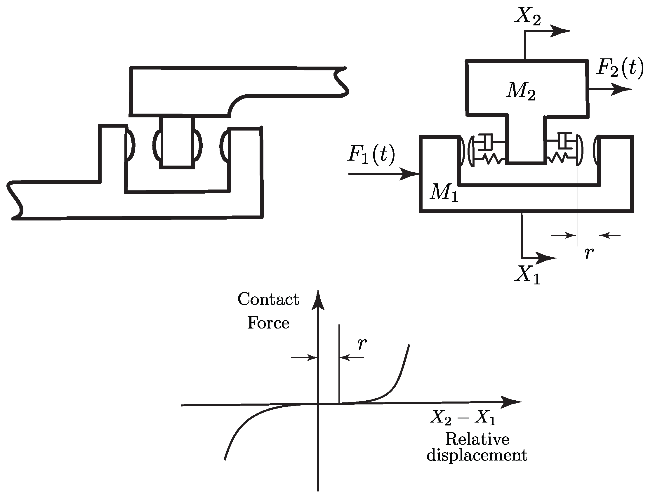
Dubowsky and Freudenstein [32,33,34] developed a systematic and unified analysis of the dynamics of general planar mechanisms with clearances. Figure 1 represents their impact-pair model governed by the following differential equations:

• Non-contact period $\left|X_r\right|\le r$

  $$\begin{array}{cc}\hfill {\ddot{X}}_r& ={\displaystyle \frac{M_1{F}_2\left(t\right)-M_2{F}_1\left(t\right)}{M_1{M}_2}}\hfill \end{array}$$

  (5a)

  $$\begin{array}{cc}\hfill {\ddot{X}}_m& ={\displaystyle \frac{M_1{F}_2\left(t\right)+M_2{F}_1\left(t\right)}{M_1{M}_2}}\hfill \end{array}$$

  (5b)
• Contact period $\left|X_r\right|\ge r$

  $$\begin{array}{cc}\hfill {\ddot{X}}_r& =-{\displaystyle \frac{M_1+M_2}{M_1{M}_2}}g\left(X_r\right)+{\displaystyle \frac{F_2\left(t\right)}{M_2}}-{\displaystyle \frac{F_1\left(t\right)}{M_1}}\hfill \end{array}$$

  (6a)

  $$\begin{array}{cc}\hfill {\ddot{X}}_m& ={\displaystyle \frac{M_2-M_1}{M_1{M}_2}}g\left(X_r\right)+{\displaystyle \frac{F_2\left(t\right)}{M_2}}+{\displaystyle \frac{F_1\left(t\right)}{M_1}}\hfill \end{array}$$

  (6b)

The contact compliance force $F_n$ was computed by means of the following Hertz contact formula:

$$F_n={\displaystyle \frac{4{\left({\displaystyle \frac{R_1{R}_2}{R_1-R_2}}\right)}^{\frac{1}{2}}}{3\left(h_1+h_2\right)}}{\delta }^{\frac{3}{2}}$$

(7)

where the indentation, for the internal-pin configuration, follows from

$$\delta =\pi \left({\displaystyle \frac{h_1+h_2}{2a}}\right)\left[ln\left({\displaystyle \frac{\left(R_1-R_2\right)8a^3}{F_n{R}_1{R}_2\pi \left(h_1+h_2\right)}}\right)+1\right]F_n$$

(8)

where a is half the length of the pin.

Figure 1. Dubowsky and Freudenstein elastic coupling model. $F_1$, $F_2$: Forces; $M_1$, $M_2$: Masses; $X_1$, $X_2$: Displacements; r: clearance [33].

Figure 1. Dubowsky and Freudenstein elastic coupling model. $F_1$, $F_2$: Forces; $M_1$, $M_2$: Masses; $X_1$, $X_2$: Displacements; r: clearance [33].

3.2. Hunt and Crossley (1975)

Hunt and Crossley [41] start by expressing the variation of the kinetic energy of a mass impacting against a stationary body as follows:

$$\begin{array}{cc}\hfill \Delta E& ={\displaystyle \frac{1}{2}}{m}_r\left(v_o^2-v_i^2\right)\hfill \\ \hfill & ={\displaystyle \frac{1}{2}}{m}_r{v}_i^2\left[1-\left(1-\alpha v_i^2\right)\right]\hfill \end{array}$$

(9)

where m is the mass of the moving body, and (The equation is valid for a Maxwell material and low values of $v_i$. See also [24], p. 368 or [23], plots on p. 259 and discussion on p. 265. The constant $\alpha$ is determined experimentally and has the dimensions of an inverse speed. Hunt and Crossley estimate a value within $\left[0.08,0.32\right]$ s/m)

$$\alpha ={\displaystyle \frac{1-e}{v_i}}$$

(10)

where e is the coefficient of restitution, and $v_i$ is the initial effective mass-relative speeds. Since $\alpha <1$, with acceptable accuracy

$$\Delta E=\alpha m_r{v}_i^3$$

(11)

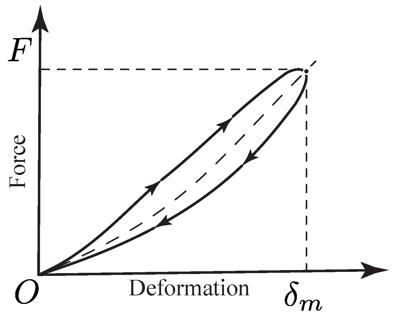
Consequently, the force versus displacement plot must show a hysteresis loop, as shown in Figure 2.

Moreover, they were well aware that the differential equation of the idealized Kelvin–Voigt model

$$m_r\ddot{\delta }+c\dot{\delta }+K\delta =0$$

(12)

could not reliably reproduce the overall nonlinear pattern of the impact. Thus, they proposed an improvement substituting (12) with

$$m_r\ddot{\delta }+\left(\lambda {\delta }^n\right)\dot{\delta }+K{\delta }^n=0$$

(13)

Moreover, they observed that for a small dissipation of energy

$${\displaystyle \frac{1}{2}}{m}_r{v}_i^2\approx {\int }_0^{{\delta }_m}K{\delta }^n\mathrm{d}\delta$$

(14)

or

$$v_i=\sqrt{{\displaystyle \frac{2K}{m_r(n+1)}}}{\delta }_m^{\frac{n+1}{2}}$$

(15)

where ${\delta }_m$ is the maximum indentation value.

Similarly, for an intermediate position of the impact phase, one has

$${\displaystyle \frac{1}{2}}{m}_r{v}^2\approx {\displaystyle \frac{1}{2}}{m}_r{v}_i^2-{\int }_0^{\delta }K{\delta }^n\mathrm{d}\delta$$

(16)

or

$$v=\sqrt{{\displaystyle \frac{2K}{m_r(n+1)}}}\sqrt{{\delta }_m^{n+1}-{\delta }^{n+1}}$$

(17)

Furthermore, assuming that the linear area of the hysteresis loop is shared sufficiently equally between the inward and outward indentation phases, one has

$$E=\oint cv\mathrm{d}\delta \approx 2{\int }_0^{{\delta }_m}cv\mathrm{d}\delta$$

(18)

or

$$\Delta E=2\sqrt{{\displaystyle \frac{2K}{m_r(n+1)}}}{\int }_0^{{\delta }_m}c\sqrt{{\delta }_m^{n+1}-{\delta }^{n+1}}\mathrm{d}\delta$$

(19)

To integrate (19), a damping coefficient of the form

$$c=\lambda {\delta }^n$$

(20)

is assumed, and the following expression is deduced

$$\lambda ={\displaystyle \frac{3}{2}}\alpha K$$

(21)

Thus, one may conclude that (12), representing the free-damped half cycle of vibration of the vibroimpact, can be more realistically modified as follows

$$m_r\ddot{\delta }+K{\delta }^n\left(1+{\displaystyle \frac{3}{2}}\alpha \dot{\delta }\right)=0$$

(22)

One of the merits of Hunt and Crossley is the recognition that a linear elastic spring cannot accurately represent the physics of the energy transfer process during the impact. Flores and Lankarani (see Section 3.1 of [25]) clearly show, with convincing arguments, the limits of the linear Kelvin–Voigt model.

In conclusion, the contact force equation proposed is the following

$$\begin{array}{|c|}\hline F_n=K{\delta }^{\frac{3}{2}}\left(1+\frac{3}{2}\frac{(1-e)}{{\dot{\delta }}^{(-)}}\dot{\delta }\right)\\ \hline\end{array}$$

(23)

Moreover, Hunt and Crossley, well aware of the theoretical limitations of the coefficient of restitution concept, recommended its use in an engineering context provided verifications and extensions for new materials and impacting surfaces properties were available. It is well known that small changes in impact conditions have a strong influence on the coefficient of restitution. Several studies (e.g.,Tatara and Moriwaki [42], Thornton [43], Seifried et al. [44], Minamoto and Kawamura) [45]) address the theoretical and experimental coefficient of restitution evaluation for the impact of bodies of different materials.

3.3. Herbert and McWhannel (1975)

Herbert and McWhannel [46] followed an approach similar to the one of Hunt and Crossley and deduced

$$\alpha =\frac{6(1-e)}{v_i\left[{(2e-1)}^2+3\right]}$$

(24)

In particular, they proposed the following formula for the contact force:

$$\begin{array}{|c|}\hline F_n=K{\delta }^{\frac{3}{2}}\left(1+\frac{6(1-e)}{\left[{(2e-1)}^2+3\right]{\dot{\delta }}^{(-)}}\dot{\delta }\right)\\ \hline\end{array}$$

(25)

For the coefficient of restitution e, Herbert and McWhannel recommended the following empirical equation:

$$e=1-0.026{\left({\dot{\delta }}^{(-)}\right)}^{\frac{1}{3}}$$

(26)

with the velocity expressed in mm/s.

3.4. Lee and Wang (1983)

Lee [47] observed that, due to their inherent kinematic limitations, Geneva mechanisms are subjected to shock loading. Moreover, pin-slot compliances, elastic deflections and imbalances interact to contribute to the dynamic load between the pin and slot. The design procedure proposed aims to minimize shock loading and contact stresses. In particular, the Hertz formula contacts a plane surface to estimate the pin-slot contact stress.

The physical model proposed by Lee and Wang [48,49] is the same as the one from Dubowsky and Freudenstein [33] (see Figure 1). For the modeling of damping, the differences regard the introduction of two new functions. The first one is apt to be evaluated by means of empirical or published experimental data. The second one is based on a heuristic choice of the damping force consistent with the boundary conditions imposed by the force-deformation hysteresis loop. The first damping function takes the form

$$D_1={\zeta }_1{T}_1$$

(27)

where ${\zeta }_1$ and $T_1$ represent the damping factor and an indentation function, respectively. The simplest choice of $T_1$ is linear:

$$T_1=\delta$$

(28)

From the fitting of experimental data, it is possible to express the coefficient of restitution e as a linear polynomial

$$e\doteq {\alpha }_0-{\alpha }_1{v}_i$$

(29)

where ${\alpha }_0$ and ${\alpha }_1$ are the polynomial coefficients and $v_i$. By definition

$$e=-{\displaystyle \frac{v_o}{v_i}}$$

(30)

The differential equation governing the indentation during the contact phase between the body surfaces can be written in the form

$$m_r\ddot{\delta }+\left({\zeta }_1\delta \right)\dot{\delta }+K\delta =P\left(t\right)$$

(31)

and its solution is obtained as polynomial approximation

$$\begin{array}{cc}\hfill \delta \left(t\right)\doteq v_{i}t -& {\displaystyle \frac{{\zeta }_1{v}_i+K}{6m_r}}{v}_i{t}^3\hfill \\ \hfill & +{\displaystyle \frac{\left(4{\zeta }_1{v}_i+K\right)\left({\zeta }_1{v}_i+K\right)v_i}{120m_r^2}}{t}^5+\dots \hfill \end{array}$$

(32)

Since the relative velocity at the end of the outward contact phase $(t=t_e)$ is

$$\begin{array}{cc}\hfill v_o=\dot{\delta }\left(t_e\right)=v_i -& {\displaystyle \frac{{\zeta }_1{v}_i+K}{2m_r}}{v}_i{t}_e^2\hfill \\ \hfill & +{\displaystyle \frac{\left(4{\zeta }_1{v}_i+K\right)\left({\zeta }_1{v}_i+K\right)v_i}{24m_r^2}}{t}_e^4+\dots \hfill \end{array}$$

(33)

The substitution of (33) into (30) yields the coefficient of restitution

$$e=-1+{\displaystyle \frac{K{t}_e^2}{2m_r}}+\left(1-{\displaystyle \frac{5K{t}_e^2}{12m_r}}\right){\displaystyle \frac{{\zeta }_1{t}_e^2}{2m_r}}{v}_i-{\displaystyle \frac{{\zeta }_1^2{t}_e^4}{6m_r^2}}{v}_i^2+\dots$$

(34)

Comparing (29) with (34), we obtain

$${\alpha }_0=-1+{\displaystyle \frac{K{t}_e^2}{2m_r}}$$

(35)

To estimate $t_e$, Lee and Wang set (This choice is consistent with the usual polynomial fitting of coefficient of restitution $e=1-{\alpha }_1{v}_i$.) ${\alpha }_0=1$ in (27) and obtained

$$t_e^2=4{\displaystyle \frac{m_r}{K}}$$

(36)

thus

$${\zeta }_1={\displaystyle \frac{2m_r}{\left({\displaystyle \frac{5K{t}_e^2}{12m_r}}-1\right)t_e^2}}{\alpha }_1\approx {\displaystyle \frac{3}{4}}{\alpha }_{1}K$$

(37)

The algebraic structure of the result matches with the one deduced by Hunt and Crossley [41] by means of an energy balance. The first damping coefficient is

$${\zeta }_1\doteq \left({\displaystyle \frac{3}{4}}{\alpha }_{1}K\right)\delta$$

(38)

In conclusion, the first contact force formula proposed by Lee and Wang is

$$\begin{array}{|c|}\hline f_n=K\delta \left(1+{\displaystyle \frac{3}{4}}{\alpha }_1\dot{\delta }\right)\\ \hline\end{array}$$

(39)

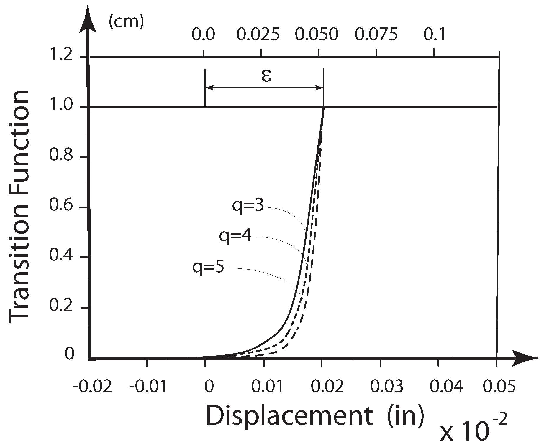
The derivation of the second damping function follows the same guidelines as the first damping function. In particular, such a function is expressed as

$$D_2={\zeta }_2{T}_2$$

(40)

where ${\zeta }_2$ is a damping factor, and

$$T_2={\displaystyle \frac{\delta +\left|\delta \right|}{2\delta }}\exp \left\{\left[\left(\delta -\epsilon \right)-\left|\delta -\epsilon \right|\right]{\displaystyle \frac{q}{\epsilon }}\right\}$$

(41)

is the transition function, with $\epsilon$ being the width of the impact transition zone (see Figure 3) and q a parameter specifying the curve path within the transition zone. Typical values of q are 2, 3 and 4.

Parameter value $\epsilon$ can be arbitrarily chosen, but the conditions

$$\begin{array}{cc}\hfill & 0\le \epsilon \le {\delta }_m\hfill \end{array}$$

(42)

$$\begin{array}{cc}\hfill & {\zeta }_2{T}_2\left(\delta \right)\dot{\delta }+K_e\delta \ge 0\hfill \end{array}$$

(43)

that ensure the sum of damping and spring forces to be positive must be fulfilled.

With a procedure similar to the one adopted for the first damping factor [50], one obtains

$${\zeta }_2=2m_r\omega \sqrt{{\displaystyle \frac{{\left(lne\right)}^2}{{\left(lne\right)}^2+{\pi }^2}}}$$

(44)

where $\omega$ is the system’s natural frequency.

It has been observed that the simulations based on the second damping function are more stable and have a hysteresis loop wider than the one predicted with the first damping function.

In conclusion, the second contact force model proposed by Lee and Wang is summarized by the following formula:

$$\begin{array}{|c|}\hline f_n=K_e\delta +{\zeta }_2{T}_2\dot{\delta }\\ \hline\end{array}$$

(45)

where $T_2$ and ${\zeta }_2$ are computed from (41) and (44), respectively.

3.5. Khulief and Shabana (1985)

The approach of Khulief and Shabana [51,52,53] is aimed to be implemented within a multibody dynamic environment and the nomenclature is thus adapted for the purpose. Their analysis is based on the assumption that the energy dissipated during the impact is much less than the elastic strain energy involved. Therefore, the coefficient of restitution is $e\approx 1$. The bodies are assimilated to point masses or with a relative translation motion.

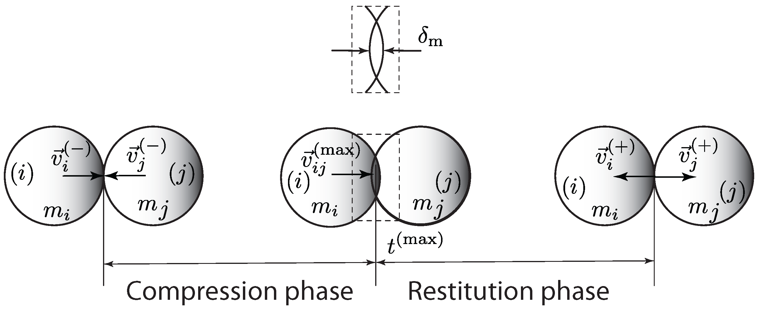
As shown in Figure 4, the collision process is divided into:

• the compression phase, during which the relative velocity ${\stackrel{.}{\delta }}_{ij}$ is gradually reduced to zero and elastic energy is stored;
• the restitution phase, which begins at the release of the stored elastic energy and finishes when the bodies separate.

Figure 4. Central collision between two circular-shaped masses: representation of the compression and restitution phase [14,25].

Figure 4. Central collision between two circular-shaped masses: representation of the compression and restitution phase [14,25].

The force between bodies i and j is analytically represented by the Kelvin–Voigt model

$$F_{ij}=\left(K{\delta }_{ij}+c{\dot{\delta }}_{ij}\right)L{G}_{ij}$$

(46)

where

$$L{G}_{ij}=\left\{\begin{array}{c}1\mathrm{during}\mathrm{impact}\hfill \\ 0\mathrm{after}\mathrm{separation}\hfill \end{array}\right.$$

(47)

is a logical function. The following nomenclature is introduced: ${\widehat{\delta }}_{ij}$ is the maximum value of indentation; ${\overline{u}}_i$ and ${\tilde{u}}_i$ are the velocities of body i at the beginning of the compression phase and at the end of the restitution phase, respectively; $u_{ij}$ is the body velocity when ${\dot{\delta }}_{ij}=0$ (end of compression phase); ${\overline{\dot{\delta }}}_{ij}={\overline{u}}_j-{\overline{u}}_i$ is the relative velocity at the beginning of compression phase.

The energy conservation principle yields:

$${\displaystyle \frac{1}{2}}{m}_i{\overline{u}}_i^2+{\displaystyle \frac{1}{2}}{m}_j{\overline{u}}_j^2={\displaystyle \frac{1}{2}}\left(m_i+m_j\right)u_{ij}^2+\underset{\mathrm{Maximum}\mathrm{strain}\mathrm{energy}}{\underbrace{{\int }_0^{{\widehat{\delta }}_{ij}}K{\delta }_{ij}\mathrm{d}{\delta }_{ij}}}$$

(48)

where

$$\begin{array}{cc}\hfill u_{ij}& ={\overline{u}}_i+\Delta {\overline{u}}_i\hfill \end{array}$$

(49a)

$$\begin{array}{cc}\hfill u_{ij}& ={\overline{u}}_j+\Delta {\overline{u}}_j\hfill \end{array}$$

(49b)

Using the momentum conservation principle, one has

$$m_i\Delta {\overline{u}}_i+m_j\Delta {\overline{u}}_j=0$$

(50)

or, taking into account (49),

$$u_{ij}=\left[{\displaystyle \frac{m_j}{m_i+m_j}}\right]{\overline{u}}_j+{\displaystyle \frac{m_i}{m_j}}{\overline{u}}_i$$

(51)

The substitution of (51) into (48), with the hypothesis of a constant contact stiffness K, gives [52]:

$${\displaystyle \frac{1}{2}}K{\delta }_{ij}^2={\displaystyle \frac{1}{2}}\left({\displaystyle \frac{m_i{m}_j}{m_i+m_j}}\right){\overline{\dot{\delta }}}_{ij}^2$$

(52)

where

$${\overline{\dot{\delta }}}_{ij}={\overline{u}}_i-{\overline{u}}_j$$

(53)

Equation (52) allows a relationship between the contact stiffness upper bound $\overline{K}$

$$\overline{K}={\displaystyle \frac{m_i{m}_j}{m_i+m_j}}{\left({\displaystyle \frac{{\overline{\dot{\delta }}}_{ij}}{{\widehat{\delta }}_{ij}}}\right)}^2$$

(54)

and the impacting bodies’ kinematics.

To obtain an expression for the damping coefficient, the kinetic energy loss $\Delta E$ and the coefficient of restitution must be taken into account.

The combination of the following three equations:

$$\begin{array}{cc}\hfill \Delta E& ={\displaystyle \frac{1}{2}}{m}_i\left({\overline{u}}_i^2-{\tilde{u}}_i^2\right)-{\displaystyle \frac{1}{2}}{m}_j\left({\overline{u}}_j^2+{\tilde{u}}_j^2\right)\mathrm{Energy}\mathrm{balance}\hfill \end{array}$$

(55)

$$\begin{array}{cc}\hfill e& =-{\displaystyle \frac{{\tilde{u}}_i-{\tilde{u}}_j}{{\overline{u}}_i-{\overline{u}}_j}}\mathrm{Coefficient}\mathrm{of}\mathrm{restitution}\hfill \end{array}$$

(56)

$$\begin{array}{cc}\hfill m_i& \left({\overline{u}}_i-{\tilde{u}}_i\right)+m_j\left({\overline{u}}_j-{\tilde{u}}_j\right)=0\mathrm{Momentum}\mathrm{conservation}\hfill \end{array}$$

(57)

gives

$$\Delta E={\displaystyle \frac{1}{2}}\left[{\displaystyle \frac{\left(1-e\right)m_i{m}_j}{m_i+m_j}}\right]{\overline{\dot{\delta }}}_{ij}^2$$

(58)

This energy loss is dissipated by the damping force expressed as $D{\dot{\delta }}_{ij}$. Therefore, it is

$$\Delta E=\oint D{\dot{\delta }}_{ij}\mathrm{d}{\delta }_{ij}$$

(59)

where ∮ denotes the integration around the force-displacement hysteresis loop.

$$\underset{\mathrm{Kinetic}\mathrm{energy}\mathrm{at}\mathrm{start}}{\underbrace{{\displaystyle \frac{1}{2}}{m}_i{\overline{u}}_i^2+{\displaystyle \frac{1}{2}}{m}_j{\overline{u}}_j^2}}=\underset{\mathrm{Energy}\mathrm{at}\mathrm{intermediate}\mathrm{time}}{\underbrace{{\displaystyle \frac{1}{2}}{m}_i{u}_i^2+{\displaystyle \frac{1}{2}}{m}_j{u}_j^2+{\int }_0^{{\delta }_{ij}}\overline{K}\mathrm{d}{\delta }_{ij}}}$$

(60)

with

$$\begin{array}{cc}\hfill u_i& ={\overline{u}}_i+\Delta u_i\hfill \end{array}$$

(61a)

$$\begin{array}{cc}\hfill u_j& ={\overline{u}}_j+\Delta u_j\hfill \end{array}$$

(61b)

From the previous one follows:

$${\dot{\delta }}_{ij}={\overline{\dot{\delta }}}_{ij}+\Delta u_i-\Delta u_j$$

(62)

Combining the momentum conservation equation

$$m_i\Delta u_i+m_j\Delta u_j=0$$

(63)

with (60) and (61), taking into account (54), one obtains:

$$\begin{array}{cc}\hfill {\int }_0^{{\delta }_{ij}}\overline{K}{\delta }_{ij}\mathrm{d}{\delta }_{ij}=& {\displaystyle \frac{1}{2}}\left({\displaystyle \frac{m_i{m}_j}{m_i+m_j}}\right)\left[{\overline{\dot{\delta }}}_{ij}^2-{\dot{\delta }}_{ij}^2\right]\hfill \end{array}$$

(64)

or

$$\overline{K}{\delta }_{ij}^2=\left({\displaystyle \frac{m_i{m}_j}{m_i+m_j}}\right)\left[{\overline{\dot{\delta }}}_{ij}^2-{\dot{\delta }}_{ij}^2\right]$$

(65)

Consequently, from (65) follows

$${\dot{\delta }}_{ij}=\sqrt{{\overline{\dot{\delta }}}_{ij}^2-\left[{\displaystyle \frac{\overline{K}\left(m_i+m_j\right)}{m_i{m}_j}}\right]{\delta }_{ij}^2}$$

(66)

Finally, the substitution of (66) into (59) and the choice of a damping function of the form (The function satisfies the boundary conditions at both the contact start and separation).

$$D=\mu {\delta }_{ij}$$

(67)

yelds (It is assumed the area of the hysteresis loop is equally shared between compression and restitution phase.

$$\Delta E=2{\int }_0^{{\widehat{\delta }}_{ij}}\mu {\delta }_{ij}\sqrt{{\overline{\dot{\delta }}}_{ij}^2-{\overline{\beta }}^2{\delta }_{ij}^2}\mathrm{d}{\delta }_{ij}$$

(68)

After we let

$${\overline{\beta }}^2={\displaystyle \frac{\overline{K}\left(m_i+m_j\right)}{m_i{m}_j}}={\left({\displaystyle \frac{{\overline{\dot{\delta }}}_{ij}}{{\widehat{\delta }}_{ij}}}\right)}^2$$

(69)

Equation (68) can be rewritten in the form

$$\Delta E=-{\displaystyle \frac{2}{3}}\mu \overline{\beta }\left\{{\left[{\left({\displaystyle \frac{{\overline{\dot{\delta }}}_{ij}}{\overline{\beta }}}\right)}^2-{\widehat{\delta }}_{ij}^2\right]}^{\frac{3}{2}}-{\left({\displaystyle \frac{{\overline{\dot{\delta }}}_{ij}}{\overline{\beta }}}\right)}^3\right\}$$

(70)

Equating (70) and (58), one obtains

$$\mu ={\displaystyle \frac{3}{4}}\left({\displaystyle \frac{\overline{K}\left(1-e^2\right){\overline{\dot{\delta }}}_{ij}^2}{\left[{\overline{\dot{\delta }}}_{ij}^2-{\left({\overline{\dot{\delta }}}_{ij}^2-{\overline{\beta }}^2{\widehat{\delta }}_{ij}^2\right)}^{\frac{3}{2}}\right]}}\right)$$

(71)

and the force-approach law, according to Khulief and Shabana [51,52,53], is expressed in the form

$$\begin{array}{|c|}\hline F_n=K{\delta }_{ij}+\left(\mu {\delta }_{ij}\right){\dot{\delta }}_{ij}\\ \hline\end{array}$$

(72)

where $\mu$ is computed from (71).

3.6. Lankarani and Nikravesh (1988)

Lankarani and Nikravesh [8,9,35] recognized the limits and inconsistencies of the Kelvin–Voigt model and proposed a contact force expressed by the following equation

$$F_n=K{\delta }^n+D\dot{\delta }$$

(73)

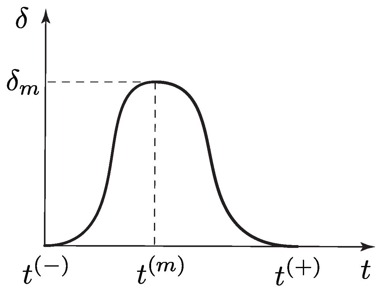
for the entire period of contact. They assumed that the energy dissipated during the impact is small compared to the maximum absorbed elastic energy. Moreover, within the contact time interval, they distinguished a compression and a restitution phase. With reference to Figure 5, let $t^{(-)}$, $t^{\left(m\right)}$ and $t^{(+)}$ denote the initial time of compression, the time of maximum indentation and the final time of restitution, respectively.

Lankarani and Nikravesh start by writing the equations expressing:

• the energy loss $\Delta E$ computed as a difference between the bodies’ kinetic energies at the beginning and at the end of the impact:

  $$\begin{array}{cc}\hfill \Delta E& =T^{(-)}-T^{(+)}\hfill \\ \hfill & ={\displaystyle \frac{m_i}{2}}\left[{\left(v_i^{(-)}\right)}^2-{\left(v_i^{(+)}\right)}^2\right]+{\displaystyle \frac{m_j}{2}}\left[{\left(v_j^{(-)}\right)}^2-{\left(v_j^{(+)}\right)}^2\right]\hfill \end{array}$$

  (74)
• the conservation of linear momentum:

  $$m_i\left[v_i^{(-)}-v_i^{(+)}\right]+m_j\left[v_j^{(-)}-v_j^{(+)}\right]=0$$

  (75)
• the coefficient of restitution:

  $$e=-{\displaystyle \frac{v_i^{(+)}-v_j^{(+)}}{v_i^{(-)}-v_j^{(-)}}}$$

  (76)

The combination of (74)–(76) gives:

$$\Delta E={\displaystyle \frac{1}{2}}{\displaystyle \frac{m_i{m}_j}{m_i+m_j}}{\left[{\dot{\delta }}^{(-)}\right]}^2\left(1-e^2\right)$$

(77)

where

$${\dot{\delta }}^{(-)}=v_i^{(-)}-v_j^{(-)}$$

(78)

Furthermore, considering the time interval $\left[t^{(-)},t^{\left(m\right)}\right]$ between the beginning and end of the compression phase, one can write:

• the energy balance equation

  $$\begin{array}{cc}\hfill T^{(-)}=& T^{\left(m\right)}+U^{\left(m\right)}\hfill \\ \hfill {\displaystyle \frac{1}{2}}{m}_i{\left[v_i^{(-)}\right]}^2+{\displaystyle \frac{1}{2}}{m}_j{\left[v_j^{(-)}\right]}^2=& {\displaystyle \frac{1}{2}}\left(m_i+m_j\right)\left[v_{ij}^{\left(m\right)}\right]+U^{\left(m\right)}\hfill \end{array}$$

  (79)
• the linear momentum conservation equation

  $$m_i{v}_i^{(-)}+m_j{v}_j^{(-)}=\left(m_i+m_j\right)v_{ij}^{\left(m\right)}$$

  (80)

The combination of (79) and (80) yields

$$U^{\left(m\right)}={\displaystyle \frac{1}{2}}\left({\displaystyle \frac{m_i{m}_j}{m_i+m_j}}\right){\left[{\dot{\delta }}^{(-)}\right]}^2$$

(81)

Such energy can also be evaluated by means of the integral

$$U^{\left(m\right)}={\int }_0^{{\delta }_m}K{\delta }^n\mathrm{d}\delta ={\displaystyle \frac{K}{n+1}}{\delta }_m^{n+1}$$

(82)

The comparison of (81) and (82) gives

$${\left[{\dot{\delta }}^{(-)}\right]}^2=2{\displaystyle \frac{\left(m_i+m_j\right)K}{m_i{m}_j(n+1)}}{\delta }_m^{n+1}$$

(83)

This relationship shows how the maximum indentation ${\delta }_m$ is influenced by the contact stiffness K and the difference in mass velocities at $t^{(-)}$.

Repeating the previous reasoning for a generic time interval $\left[t^{(-)},t\right]$, with $t^{(-)}\le t\le t^{\left(m\right)}$, one obtains

$${\dot{\delta }}^2={\left[{\dot{\delta }}^{(-)}\right]}^2-2{\displaystyle \frac{m_i+m_j}{m_i{m}_j}}{\displaystyle \frac{K{\delta }^{n+1}}{n+1}}$$

(84)

With (84), the energy dissipated by the damping force is computed by means of the integral (It is assumed the area of the hysteresis loop is equally shared between the compression and restitution phase.):

$$\Delta T=\oint D\dot{\delta }\mathrm{d}\delta =\oint \mu {\delta }^n\dot{\delta }\mathrm{d}\delta =2{\int }_0^{{\delta }_m}\mu {\delta }^n\dot{\delta }\mathrm{d}\delta$$

(85)

or, taking into account (83) and (84),

$$\Delta E={\displaystyle \frac{2\mu }{3K}}{\displaystyle \frac{m_i{m}_j}{m_i+m_j}}{\left[{\dot{\delta }}^{(-)}\right]}^3$$

(86)

The comparison of (77) and (86) yields

$$\mu ={\displaystyle \frac{3K\left(1-e^2\right)}{4{\dot{\delta }}^{(-)}}}$$

(87)

and the contact force is finally expressed by the following formula:

$$\begin{array}{|c|}\hline F_n=K{\delta }^n\left[1+{\displaystyle \frac{3\left(1-e^2\right)}{4}}{\displaystyle \frac{\dot{\delta }}{{\dot{\delta }}^{(-)}}}\right]\\ \hline\end{array}$$

(88)

3.7. Tsuji et al. (1992)

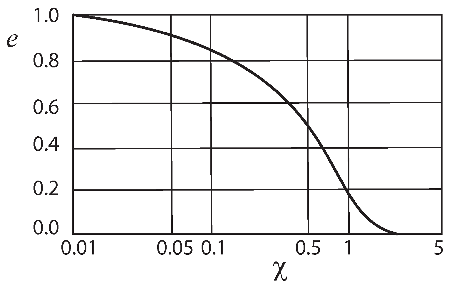
Tsuji et al. [54] assumed the indentation during the contact governed by the following differential equation:

$$m_r\ddot{\delta }+c\dot{\delta }+K{\delta }^{\frac{3}{2}}=0$$

(89)

The damping coefficient equation

$$c=\chi {\delta }^{\frac{1}{4}}\sqrt{m_{r}K}$$

(90)

has been found heuristically. Parameter $\chi$ is an empirical constant related to the coefficient of restitution, as shown in Figure 6.

3.8. Lankarani and Nikravesh (1994)

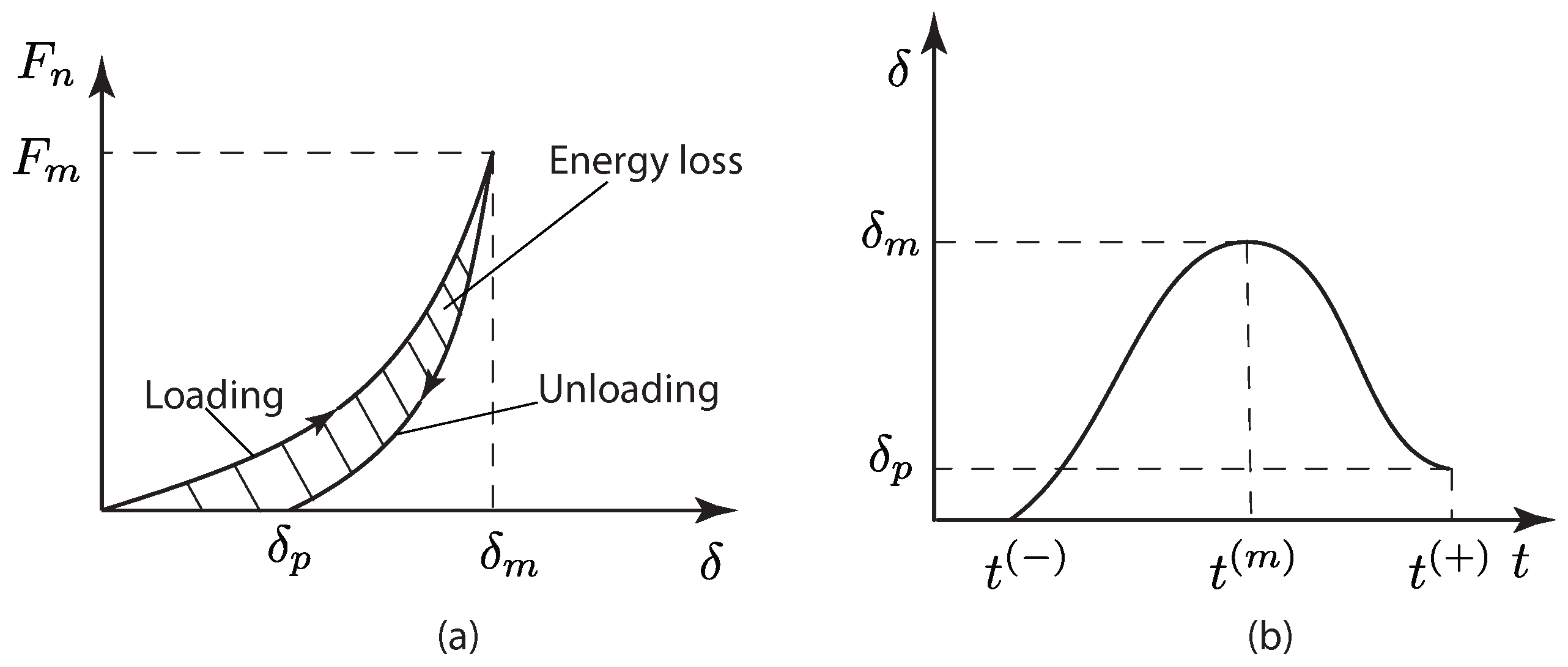
Lankarani and Nikravesh [55] extended their analysis to the case where, after the impact between two spheres, a permanent indentation ${\delta }_p$ due to local plasticity is observed (see Figure 7). Such a circumstance is realistic during the collision of metallic bodies with an initial relative velocity larger than ${10}^{-5}{V}_s$, where $V_s$ is the elastic wave propagation speed in the colliding bodies.

The contact force changes according to the following equation:

$$\begin{array}{|c|}\hline F_n=\left\{\begin{array}{cc}K{\delta }^n\hfill & \mathrm{compression}\mathrm{phase}\hfill \\ F_m{\left({\displaystyle \frac{\delta -{\delta }_p}{{\delta }_m-{\delta }_p}}\right)}^n\hfill & \mathrm{restitution}\mathrm{phase}\hfill \end{array}\right.\\ \hline\end{array}$$

(91)

As it will be shown, parameters ${\delta }_m$, $F_m$ and ${\delta }_p$ are computed by means of (94), (95) and (97), respectively.

To determine ${\delta }_m$ and $F_m$, we use the equation of motion of the two spheres in contact

$$m_r\ddot{\delta }+K{\delta }^n=0$$

(92)

when integrated with the initial conditions ${\delta }^{(-)}=0$, ${\dot{\delta }}^{(-)}=v_i^{(-)}-v_j^{(-)}$, yields:

$${\displaystyle \frac{1}{2}}{m}_r\left[{\dot{\delta }}^2-{\dot{\delta }}^{(-)2}\right]=K{\displaystyle \frac{{\delta }^{n+1}}{n+1}}$$

(93)

At the instant of maximum compression $\dot{\delta }=0$ and $\delta ={\delta }_m$. Thus, from (93), one obtains the maximum indentation:

$${\delta }_m={\left[{\displaystyle \frac{n+1}{2K}}{m}_r{\dot{\delta }}^{(-)2}\right]}^{\frac{1}{n+1}}$$

(94)

and maximum contact force

$$F_m=K{\delta }_m^n$$

(95)

The comparison of the dissipated energy, computed by means of the integration of the contact force, is

$$\Delta T={\int }_0^{{\delta }_m}K{\delta }^n\mathrm{d}\delta +{\int }_{{\delta }_m}^{{\delta }_p}{F}_m{\left[\frac{\delta -{\delta }_p}{{\delta }_m-{\delta }_p}\right]}^n\mathrm{d}\delta =\frac{F_m{\delta }_p}{n+1}$$

(96)

and (77) yields the permanent indentation

$${\delta }_p=\frac{(n+1)m_r{\dot{\delta }}^{{(-)}^2}}{2F_m}\left(1-e^2\right)$$

(97)

In conclusion, the contact force is expressed by (91), where ${\delta }_m$, $F_m$ and ${\delta }_p$ are expressed by (94), (95) and (97), respectively.

Lankarani and Shivaswamy [56,57] conducted experiments impacting a hardened steel indentor against aluminum and steel plates. The hysteresis loop in the plot of contact-force versus indentation has been experimentally obtained and compared with simulation results.

Rhee and Akay [58] describe the motion of a four-bar rocker described by three sets of equations:

• the sliding mode, when the pin and journal are in contact;
• free-flight mode, when the pin motion is governed by its own inertia and acting forces;
• impact mode, when the pin and journal begin contact.

3.9. Marhefka and Orin (1999)

Marhefka and Orin [59] obtained the same result as Hunt and Crossley but by means of different analytical reasoning. They started assuming the relative motion between masses at contact governed by the differential equation

$$m_r\ddot{\delta }+\lambda {\delta }^n\dot{\delta }+K{\delta }^n=0$$

(98)

or

$$\ddot{\delta }=\mathsf{\Lambda }{\delta }^n\dot{\delta }+\tilde{K}{\delta }^n$$

(99)

where $\tilde{K}=-{\displaystyle \frac{K}{m_r}}$ and $\mathsf{\Lambda }=-{\displaystyle \frac{\lambda }{m_r}}$.

Introducing the new variable $v=\dot{\delta }$, (99) can be rewritten in the form

$${\displaystyle \frac{\mathrm{d}v}{\mathrm{d}\delta }}=\frac{(\mathsf{\Lambda }v+\tilde{K}){\delta }^n}{v},$$

(100)

or

$$\int {\displaystyle \frac{v\mathrm{d}v}{(\mathsf{\Lambda }v+\tilde{K})}}=\int {\delta }^n\mathrm{d}\delta$$

(101)

The integration of (101), with initial conditions $\delta \left(0\right)=0$, $v\left(0\right)=v_i$, gives:

$$\mathsf{\Lambda }v-\tilde{K}ln\left|\tilde{K}+\mathsf{\Lambda }v\right|=\frac{1}{n+1}{\mathsf{\Lambda }}^2{\delta }^{n+1}+\mathsf{\Lambda }{v}_i-\tilde{K}ln\left|\tilde{K}+\mathsf{\Lambda }{v}_i\right|$$

(102)

or

$$\begin{array}{cc}\hfill \mathsf{\Lambda }v& -\tilde{K}ln\left|1+{\displaystyle \frac{\mathsf{\Lambda }}{\tilde{K}}}v\right|\hfill \\ \hfill & =\frac{1}{n+1}{\mathsf{\Lambda }}^2{\delta }^{n+1}+\mathsf{\Lambda }{v}_i-\tilde{K}ln\left|1+{\displaystyle \frac{\mathsf{\Lambda }}{\tilde{K}}}{v}_i\right|\hfill \end{array}$$

(103)

Since the values of $\alpha v_i$, ${\displaystyle \frac{\mathsf{\Lambda }v}{\tilde{K}}}$ and ${\displaystyle \frac{\mathsf{\Lambda }{v}_i}{\tilde{K}}}$ are $\ll 1$, (103) can be expanded in Taylor series such that

$$ln|1+ϵ|=ϵ-\frac{{ϵ}^2}{2}+\frac{{ϵ}^3}{3}+\dots$$

(104)

For (See also Equation (10)) $\delta =0$, $v=-e{v}_i=-\left(1-\alpha v_i\right)v_i$, solving the Taylor expansion for $\mathsf{\Lambda }$ yields:

$$\mathsf{\Lambda }\approx \frac{3\alpha \tilde{K}\left(2-\alpha v_i\right)}{2\left(2-3\alpha v_i+3{\alpha }^2{v}_i^2-{\alpha }^3{v}_i^3\right)}$$

(105)

The result of Hunt and Crossley, as expressed in Equation (21), can also be deduced from (105) assuming negligible $\alpha v_i$. After substitution of $\mathsf{\Lambda }={\displaystyle \frac{3}{2}}\alpha \tilde{K}$, from the integration of (103), one obtains the deformation of $\delta$ related to velocity $\dot{\delta }$ as follows

$$\delta ={\left(\frac{-2m_r(n+1)}{9K{\alpha }^2}\right)}^{\frac{1}{n+1}}{\left(3\alpha \left(v-v_i\right)+2ln\left|\frac{2+3\alpha v_i}{2+3\alpha v}\right|\right)}^{\frac{1}{n+1}}$$

(106)

In conclusion, the following contact force equation was proposed:

$$F_n=K{\delta }^{\frac{3}{2}}\left(1+\frac{3\alpha \left(2-\alpha v_i\right)}{2\left(2-3\alpha v_i+3{\alpha }^2{v}_i^2-{\alpha }^3{v}_i^3\right)}\right)\dot{\delta }$$

(107)

to be simplified into

$$\begin{array}{|c|}\hline F_n=K{\delta }^{\frac{3}{2}}\left(1+\frac{3\alpha \left(2-\alpha v_i\right)}{2\left(2-3\alpha v_i\right)}\right)\dot{\delta }\\ \hline\end{array}$$

(108)

neglecting the powers of $\alpha v_i$ equal to or greater than two.

3.10. Ghontier et al. (2004)

For Ghontier et al. [60] the differential equation governing the contact is

$$m_r\ddot{\delta }+K{\delta }^n(1+\alpha \dot{\delta })=0$$

(109)

where

$$\alpha ={\displaystyle \frac{K}{\lambda }}$$

(110)

To avoid tensile forces, the following inequality is required

$$1+\alpha \dot{\delta }\ge 0\forall \dot{\delta }$$

(111)

After the integration of (109), one obtains

$${\int }_{v_i}^{v_o}\frac{\dot{\delta }}{1+\alpha \dot{\delta }}\mathrm{d}\dot{\delta }+{\displaystyle \frac{K}{m_r}}{\int }_{{\delta }_{\mathrm{i}}}^{{\delta }_{\mathrm{o}}}{\delta }^n\mathrm{d}\delta =0$$

(112)

where ${\delta }_i={\delta }_o=0$ are the initial and final penetration depths, respectively.

The algebraic development of (112), taking into account the definition of kinematic coefficient of restitution (30), yields:

$$\alpha v_i-ln\left(1+\alpha v_i\right)+e\alpha v_i+ln\left(1-e\alpha v_i\right)=0$$

(113)

After we introduce the new variable

$$d=\alpha v_{i}e$$

(114)

Equation (113) can be expressed in the following form

$${\displaystyle \frac{1+{\displaystyle \frac{d}{e}}}{1-d}}=\exp \left[d\left(1+{\displaystyle \frac{1}{c}}\right)\right]$$

(115)

which is more amenable for the solution with respect to d.

In conclusion, the force contact formula proposed by Ghontier et al. is

$$\begin{array}{|c|}\hline F_n=K{\delta }^n\left(1+\alpha \dot{\delta }\right)\\ \hline\end{array}$$

(116)

where, given e and $v_i$, the damping factor $\alpha$ is obtained from (114), after the solution of (115) with respect to d. In the numerical solution of (115), one should observe that:

• $d<1$, a good initial guess is $d=1-e^2$;
• the solution must be consistent with (110);
• the solution $d_{HC}$ corresponding to the model of Hunt and Crossley is $d_{HC}={\displaystyle \frac{3}{4}}e(1-e)$.

3.11. Flores et al. (2011–2016)

Flores et al. [14,25] closely followed the work of Lankarani and Nikravesh [35]. One of the novelties of their work is distinguishing between the energy $\Delta E_c$, dissipated in the compression phase, and $\Delta E_r$, dissipated in the restitution phase:

$$T^{(-)}=T^{\left(m\right)}+U^{\left(m\right)}+\Delta E_c$$

(117)

For this purpose, they assumed that, during masses contact, the system dynamics are governed by the differential equation

$$m_r\ddot{\delta }+c\dot{\delta }+K\delta =0$$

(118)

This, neglecting damping, allowed the expression of the velocity of deformation during the two phases, respectively, as follows:

$$\begin{array}{cc}\hfill \dot{\delta }& ={\dot{\delta }}^{(-)}\sqrt{1-{\left(\frac{\delta }{{\delta }_m}\right)}^2}\hfill \\ \hfill \dot{\delta }& ={\dot{\delta }}^{(+)}\sqrt{1-{\left(\frac{\delta }{{\delta }_m}\right)}^2}\hfill \end{array}$$

(119)

where ${\delta }_m={\displaystyle \frac{{\dot{\delta }}^{(-)}}{\omega }}$ and $\omega =\sqrt{{\displaystyle \frac{K}{m_r}}}$.

Moreover, they established the mathematical relationship

$${\left(\frac{\delta }{{\delta }_m}\right)}^2+{\left(\frac{\dot{\delta }}{{\dot{\delta }}^{(-)}}\right)}^2=1$$

(120)

Since

$$\begin{array}{c}\Delta E_c={\int }_0^{{\delta }_m}\lambda {\delta }^{\frac{3}{2}}{\dot{\delta }}^{(-)}\sqrt{1-{\left(\frac{\delta }{{\delta }_m}\right)}^2}\mathrm{d}\delta \\ \Delta E_r={\int }_0^{{\delta }_m}\lambda {\delta }^{\frac{3}{2}}\left|{\dot{\delta }}^{(+)}\right|\sqrt{1-{\left(\frac{\delta }{{\delta }_m}\right)}^2}\mathrm{d}\delta \end{array}$$

(121)

with $\lambda$ parameter to be determined, the total dissipated energy is computed as follows:

$$\begin{array}{cc}\hfill \Delta E& =\Delta E_c+\Delta E_r\hfill \\ & =\chi \left({\dot{\delta }}^{(-)}+\left|{\dot{\delta }}^{(+)}\right|\right){\int }_0^{{\delta }_m}{\delta }^{\frac{3}{2}}\sqrt{1-{\left(\frac{\delta }{{\delta }_m}\right)}^2}\mathrm{d}\delta \hfill \end{array}$$

(122)

A numerical evaluation of the integral provides

$$\Delta E=\frac{1}{4}\lambda \left(1+e\right){\dot{\delta }}^{(-)}{\delta }_m^{\frac{5}{2}}$$

(123)

Finally, the combined use of Equations (77) and (123), energy balance

$$\frac{1}{2}{m}_i{\left(v_i^{(-)}\right)}^2+\frac{1}{2}{m}_j{\left(v_j^{(-)}\right)}^2=\frac{1}{2}\left(m_i+m_j\right)v_{ij}^{\left(m\right)}+\frac{2}{5}K{\delta }_m^{\frac{5}{2}}+\frac{1}{4}\lambda {\dot{\delta }}^{(-)}{\delta }_m^{\frac{5}{2}}$$

(124)

and linear momentum conservation

$$m_i{v}_i^{(-)}+m_j{v}_j^{(-)}=\left(m_i+m_j\right)v_{ij}^{\left(m\right)}$$

(125)

yields:

$$\lambda ={\displaystyle \frac{8K\left(1-e\right)}{5e{\dot{\delta }}^{(-)}}}$$

(126)

and the proposed contact force formula is as follows:

$$\begin{array}{|c|}\hline F_n=K{\delta }^{\frac{3}{2}}\left(1+\frac{8\left(1-e\right)}{5e{\dot{\delta }}^{(-)}}\dot{\delta }\right)\\ \hline\end{array}$$

(127)

Machado et al. embodied (127) in a general methodology for 3D-contact problems [61] and in biomechanic analyses of knee joints [62,63]

3.12. Gharib and Hurmuzlu (2012)

Gharib and Hurmuzlu [64] assumed a contact force of the form:

$$F_n=K{\delta }^n+\lambda {\delta }^n\dot{\delta }$$

(128)

and observed that, at the end of an elastic collision ($t=t^{(+)}$), both the contact force $F_N$ and the indentation ${\delta }_f$ vanish, while the indentation velocity is

$${\dot{\delta }}^{(+)}=v_i^{(+)}-v_j^{(+)}\ne 0$$

(129)

Therefore, the following equation holds

$${\delta }_f^n\left(K+\lambda {\dot{\delta }}^{(+)}\right)=0$$

(130)

the solution of which is

$${\dot{\delta }}^{(+)}=-{\displaystyle \frac{K}{\lambda }}$$

(131)

Since by definition of coefficient of restitution

$${\dot{\delta }}^{(+)}=-e{\dot{\delta }}^{(-)}$$

(132)

one has the following expression for the damping coefficient

$$\lambda ={\displaystyle \frac{1}{e}}{\displaystyle \frac{K}{{\dot{\delta }}^{(-)}}}$$

(133)

In conclusion, the first formula for the elastic contact force proposed by Gharib and Hurmuzlu is

$$\begin{array}{|c|}\hline F_n=K{\delta }^n\left(1+{\displaystyle \frac{\dot{\delta }}{e{\dot{\delta }}^{(-)}}}\right)\\ \hline\end{array}$$

(134)

Gharib and Hurmuzlu also analyzed the case of impact with indentation. The contact forces can be mathematically written as follows:

$$\begin{array}{cc}\hfill F_c& =K_c{\delta }^n\mathrm{compression}\mathrm{force}\hfill \end{array}$$

(135)

$$\begin{array}{cc}\hfill F_r& =F_m{\left[{\displaystyle \frac{\delta -{\delta }_p}{{\delta }_m-{\delta }_p}}\right]}^n\mathrm{restitution}\mathrm{force}\hfill \end{array}$$

(136)

The restitution force can be alternatively expressed in the form:

$$F_r=K_r{\left(\delta -{\delta }_p\right)}^n$$

(137)

Since

$$F_m\equiv K_c{\delta }_m^n=K_r{\left({\delta }_m-{\delta }_p\right)}^n$$

(138)

or

$${\delta }_p={\delta }_m\left[1-{\left(\frac{K_c}{K_r}\right)}^{\frac{1}{n}}\right]$$

(139)

Since

$${\int }_0^{{\delta }_m}{F}_c\mathrm{d}\delta =\frac{K_c{\delta }_m^{n+1}}{n+1}\mathrm{Work}\mathrm{in}\mathrm{the}\mathrm{compression}\mathrm{phase}$$

(140)

$${\int }_{{\delta }_m}^{{\delta }_p}{F}_{r}d\delta =\frac{K_r{\left({\delta }_m-{\delta }_p\right)}^{n+1}}{n+1}\mathrm{Work}\mathrm{in}\mathrm{the}\mathrm{restitution}\mathrm{phase}$$

(141)

using the definition of the energetic coefficient of restitution $e_w$ one obtains

$$e_w^2=-{\displaystyle \frac{{\int }_0^{{\delta }_m}{F}_c\mathrm{d}\delta }{{\int }_{{\delta }_m}^{{\delta }_p}{F}_r\mathrm{d}\delta }}={\left(\frac{K_c}{K_r}\right)}^{\frac{1}{n}}$$

(142)

The combination of (139) and (142) gives

$${\delta }_p={\delta }_m\left[1-e_w^2\right]$$

(143)

Moreover, the combination of (136) and (137) yields

$$K_r={\displaystyle \frac{K_c}{e_w^{2n}}}={\displaystyle \frac{F_m}{{\left({\delta }_m-{\delta }_p\right)}^n}}$$

(144)

In conclusion, for the case of impact with indentation, the second contact force formula proposed by Gharib and Hurmuzlu is

$$\begin{array}{|c|}\hline F_n=\left\{\begin{array}{cc}{K}_c{\delta }^n\hfill & \mathrm{Compression}\mathrm{phase}\hfill \\ K_r{\left(\delta -{\delta }_p\right)}^n\hfill & \mathrm{Restitution}\mathrm{phase}\hfill \end{array}\right.\\ \hline\end{array}$$

(145)

with $K_c=K$, $K_r$, $F_m$ and ${\delta }_p$ from (144), (139) and (138), respectively.

For the impact of a slender bar against a hard wall, experimental values of the coefficient of restitution are reported in [65].

3.13. Hu and Guo (2015)

Hu and Guo [66] estimate the energy loss by means of (79), whereas the relationship between the deformation and deformation velocity are

$$\dot{\delta }=\left\{\begin{array}{cc}{\dot{\delta }}^{(-)}\sqrt{1-{\left({\displaystyle \frac{\delta }{{\delta }_m}}\right)}^{\frac{5}{2}}}\hfill & \mathrm{Compression}\mathrm{phase}\hfill \\ {\dot{\delta }}^{(+)}\sqrt{1-{\left({\displaystyle \frac{\delta }{{\delta }_m}}\right)}^{\frac{5}{2}}}\hfill & \mathrm{Restitution}\mathrm{phase}\hfill \end{array}\right.$$

(146)

deduced assuming the differential Equation (2) of the elastic Hertz contact model and symmetry of behavior between compression and restitution phases.

Flores et al. [14,25] instead deduced (119) using a linear differential equation without damping.

The energy losses for the two phases are, respectively:

$$\begin{array}{c}\hfill \Delta E_c={\int }_0^{{\delta }_m}\lambda {\delta }^{\frac{3}{2}}{\dot{\delta }}^{(-)}\sqrt{1-{\left({\displaystyle \frac{\delta }{{\delta }_m}}\right)}^{\frac{5}{2}}}\mathrm{d}\delta =\frac{4}{15}\lambda {\dot{\delta }}^{(-)}{\delta }_m^{\frac{5}{2}}\end{array}$$

(147a)

$$\begin{array}{c}\hfill \Delta E_r={\int }_0^{{\delta }_m}\lambda {\delta }^{\frac{3}{2}}\left|{\dot{\delta }}^{(+)}\right|\sqrt{1-{\left({\displaystyle \frac{\delta }{{\delta }_m}}\right)}^{\frac{5}{2}}}\mathrm{d}\delta =\frac{4}{15}\lambda \left|{\dot{\delta }}^{(+)}\right|{\delta }_m^{\frac{5}{2}}\end{array}$$

(147b)

and the overall energy loss is

$$\Delta E=\Delta E_c+\Delta E_r=\Delta E=\frac{4}{15}\lambda (1+e){\dot{\delta }}^{(-)}{\delta }_m^{\frac{5}{2}}$$

(148)

To evaluate the hysteresis damping factor $\lambda$, the combination of energy balance

$$T^{(-)}=T^{\left(m\right)}+{\int }_0^{{\delta }_m}K{\delta }^{\frac{3}{2}}\mathrm{d}\delta +\Delta E_c$$

(149)

and momentum conservation (80) yields

$${\delta }_m^{\frac{5}{2}}=\frac{15m}{4\left(2\lambda {\dot{\delta }}^{(-)}+3K\right)}{\dot{\delta }}^{{(-)}^2}$$

(150)

or

$$\lambda =\frac{3K(1-e)}{2e{\dot{\delta }}^{(-)}}$$

(151)

In conclusion, Hu and Guo proposed the following formula for the normal contact force

$$\begin{array}{|c|}\hline F_n=K{\delta }^n\left[1+\frac{3(1-e)}{2e}\frac{\dot{\delta }}{\dot{\delta }(-)}\right]\\ \hline\end{array}$$

(152)

4. Numerical Example

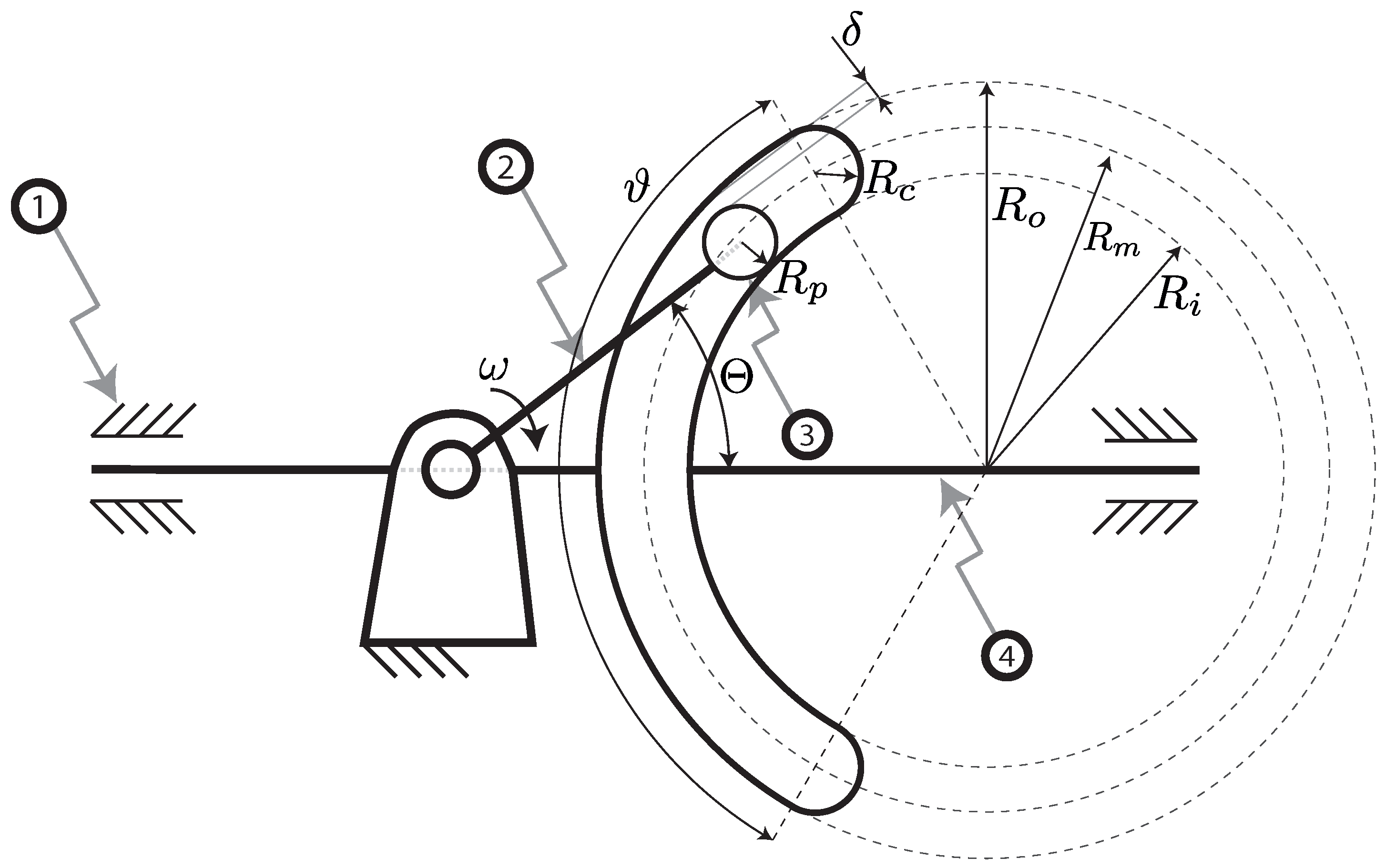
Some of the contact force models listed in the previous section have been tested within a multibody dynamics simulation. In particular, the scotch-yoke linkage with a circular guide, depicted in Figure 8, has been chosen as a test bench. In order to highlight the effect of different formulations for the normal contact force $F_n$, the only clearance introduced is the one between the pin and the circular slot. All the remaining kinematic joints are frictionless and without clearance.

The geometrical data, initial condition and inertia parameters are listed in

Table 10. Input data.

Geometry			Inertia				Initial Conditions
				Name	Mass (kg)	Inertia (kg· ${\mathbf{mm}}^2$)
$R_o$	68	mm	1	Frame	\\	\\	${\Theta }_{in}$	31	deg
$R_m$	60	mm	2	Crank	0.090	30.40	${\omega }_{in}$	0	$\frac{\mathrm{rad}}{\mathrm{s}}$
$R_i$	52	mm	3	Pin	0.015	0.48	$\omega$	$24\cdot \pi$	$\frac{\mathrm{rad}}{\mathrm{s}}$
$R_c$	8	mm	4	Slotted slider	0.353	3495.6
$R_p$	7.9	mm
$\theta$	120	deg

. The crank rotates at a constant angular speed of $24\pi \frac{\mathrm{rad}}{\mathrm{s}}$, and the effect of gravity is omitted. All bodies are made of steel with a Young modulus of 207 GPa and a Poisson ratio of $0.3$. The mechanism moves two masses m of 1 kg each fixed at both ends of the slotted slider.

As already been pointed out in the previous sections, the normal force models are mostly implicit. To reduce the computational burden of the simulation, all the formulations are represented as a polynomial function of the type $F_n=K{\delta }^n$.

The contact between the pin and circular slot has variable stiffness properties depending on the geometry bodies in contact. Three different regions can be observed:

• Pin to inner track: external contact between the pin with radius $R_p$ and the inner track with radius $R_i$;
• Pin to outer track: internal contact between the pin with radius $R_p$ and the outer track with radius $R_o$;
• Pin to circular track: internal contact between the pin with radius $R_p$ and the circumferential track with radius $R_c$.

The normal contact force is governed by the equation:

$$F_n=K{\delta }^n+\frac{3}{2}\alpha K{\left|\delta \right|}^n{\dot{\delta }}^m$$

(153)

The elastic constant K and the indentation exponent n are obtained by fitting five different cylindrical contact force relationships. In particular, the models tested are: Radzimowsky, Johnson, Goldsmith, EDSU-78035 and Lankarani and Nikravesh. Among those considered in this numerical example, the last one is the only model already explicit.

Table 11. Fitting results.

	ΔR	Lankarani		Radzimowsky		Johnson
	(mm)	K [$\frac{N}{m{m}^n}$]	n	K [$\frac{\mathrm{N}}{{\mathrm{mm}}^n}$]	n	K [$\frac{\mathrm{N}}{{\mathrm{mm}}^n}$]	n
$R_i/R_p$	$60.1$	$1.220\cdot {10}^5$	$1.50$	$4.321\cdot {10}^4$	$1.09$	$4.914\cdot {10}^4$	$1.10$
$R_o/R_p$	$59.9$	$1.424\cdot {10}^5$	$1.50$	$4.315\cdot {10}^4$	$1.09$	$4.907\cdot {10}^4$	$1.10$
$R_c/R_p$	$0.1$	$1.198\cdot {10}^6$	$1.50$	$1.846\cdot {10}^5$	$1.22$	$3.147\cdot {10}^5$	$1.28$
	ΔR	Goldsmith		EDSU-78035
	(mm)	K [$\frac{\mathrm{N}}{{\mathrm{mm}}^n}$]	n	K [$\frac{\mathrm{N}}{{\mathrm{mm}}^n}$]	n
$R_i/R_p$	$60.1$	$1.717\cdot {10}^4$	$1.04$	$1.300\cdot {10}^4$	$1.09$
$R_o/R_p$	$59.9$	$1.743\cdot {10}^4$	$1.04$	$1.254\cdot {10}^4$	$1.09$
$R_c/R_p$	$0.1$	$2.221\cdot {10}^4$	$1.05$	$4.786\cdot {10}^4$	$1.22$

reports the polynomial fitting results for each model and every contact region.

On the other hand, following the Hunt and Crossley model, the viscous coefficient C is taken proportional to K by means of the coefficient $\alpha$. For materials such as steel, bronze and ivory, Hunt and Crossley suggest values of alpha between 0.002 and 0.008 s/in (0.08–0.32 s/m). In this numerical example, $\alpha$ is set as equal to 0.32 s/m, and the penetration velocity exponent m is set to unit value.

As it is possible to observe from the fitting results, the values of K for the inner track region ($R_i$ to $R_p$) and the outer track region ($R_o$ to $R_p$) are very similar, especially for Johnson and Radzimowsky formulations. In fact, these models give the same force result for internal and external contact with the same $\Delta R$.

To clarify this statement, both the formulation of Johnson and Radzimowsky are reported below, emphasizing the $\Delta R$ dependence

$$\begin{array}{c}\hfill \delta =\frac{W}{\pi E^{*}}\left[ln\left(\frac{4\pi \Delta R{E}^{*}}{W}\right)-1\right],\mathrm{Johnson}\\ \hfill \delta =\frac{W}{\pi E^{*}}\left[\frac{2}{3}+ln\left(\frac{8\Delta R{E}^{*}}{1.6^{2}W}\right)\right],\mathrm{Radzimowsky}\end{array}$$

In the slot without clearance condition, referring to Figure 9, and minding that $\Delta R=R_i\pm R_j$ (+/−: external/internal contact), one can write:

$$\begin{array}{cc}\hfill \Delta R_{ext}& =R_p^{*}+R_i\hfill \\ \hfill \Delta R_{int}& =R_o-R_p^{*}=R_i+2R_p^{*}-R_p^{*}=R_i+R_p^{*}=\Delta R_{ext}\hfill \end{array}$$

This relationship, valid for pin-slot coupling without clearance, can be generalized with a clearance $\delta$ as

$$\Delta R_{ext}=\Delta R_{int}+\delta$$

This geometrical condition can be used to simplify the dynamic analysis of curved slots, calculating just one of the two values of K and using it for both the inner and outer track. As highlighted in Figure 10a for steel and Figure 10b for aluminum-like material, the error involved in such a simplification will be proportional to the clearance. The penetration reported is computed for a contact force per unit length of 10 $\mathrm{kN}/\mathrm{mm}$ and variable clearance. The error does not exceed 2%. This supports the righteousness of considering only one stiffness coefficient when the clearance is quite small.

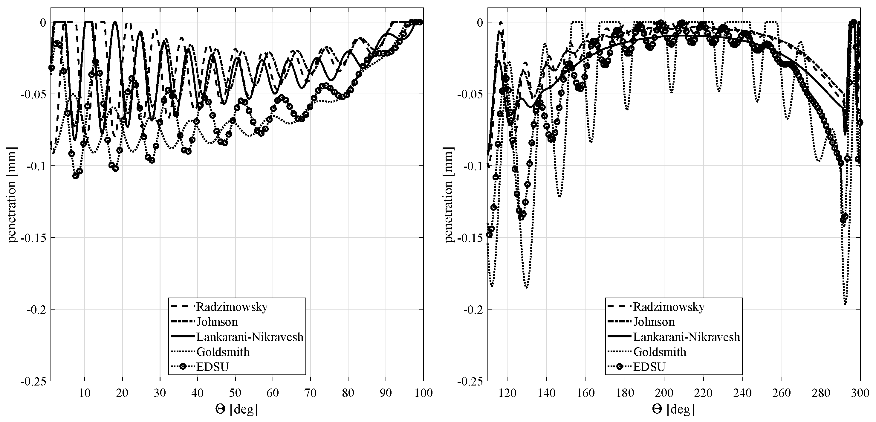
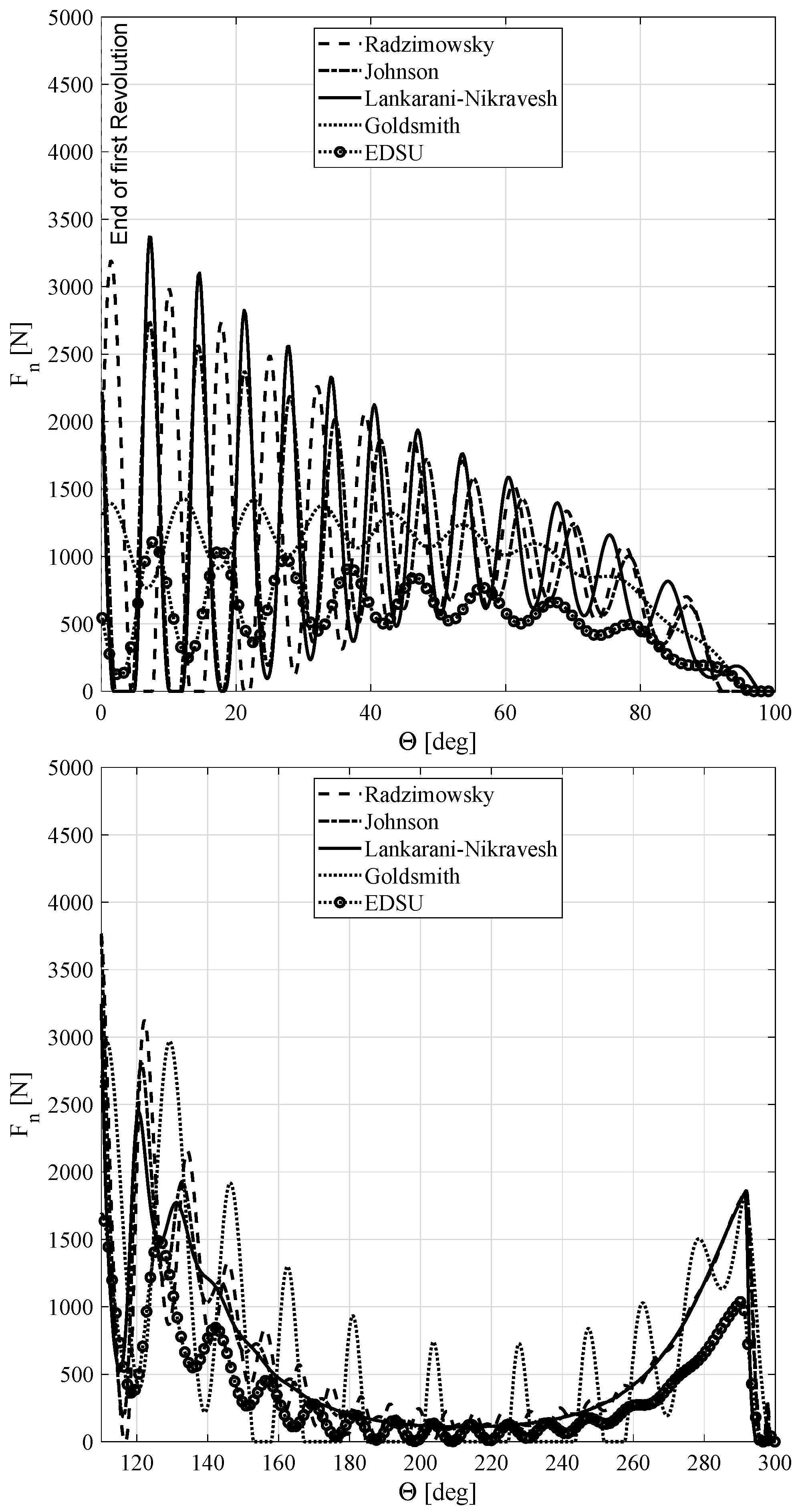
For a complete crank rotation, the comparison of contact forces computed according to the different models is depicted in Figure 11. To minimize the effects of the initial conditions, the second full crank revolution is monitored. A region with a null contact force is visible around 100 degrees of the relative crank angle corresponding to pin-slot separation caused by clearance.

When the contact is continuous (i.e., neither impact nor rebound occur), there is no relevant difference between the models. In fact, the contact force must be consistent with the dynamic equilibrium matching all the other forces acting on the system. On the other hand, the penetration, as well as its oscillation frequency, heavily depends on the contact model due to the different stiffness characteristics, as observed in Figure 12 and Figure 13.

The detail on the impact sections, depicted in Figure 14, is useful to highlight the differences in the model’s dynamic behavior. Since the exponent n values are close for all models, except for the Lankarani–Nikravesh model, one can state (for all the remaining formulations) that the higher the K value, the higher the amplitude of contact forces during the impact phases (i.e., until 100 deg of relative crank angle). Moreover, a high value of K, and, consequently, a high value of C, provides contact steadiness. In this regard, the Goldsmith model (the less stiff) is the only model that shows the detachment of the pin from the slot in the range between 120 and 300 degrees.

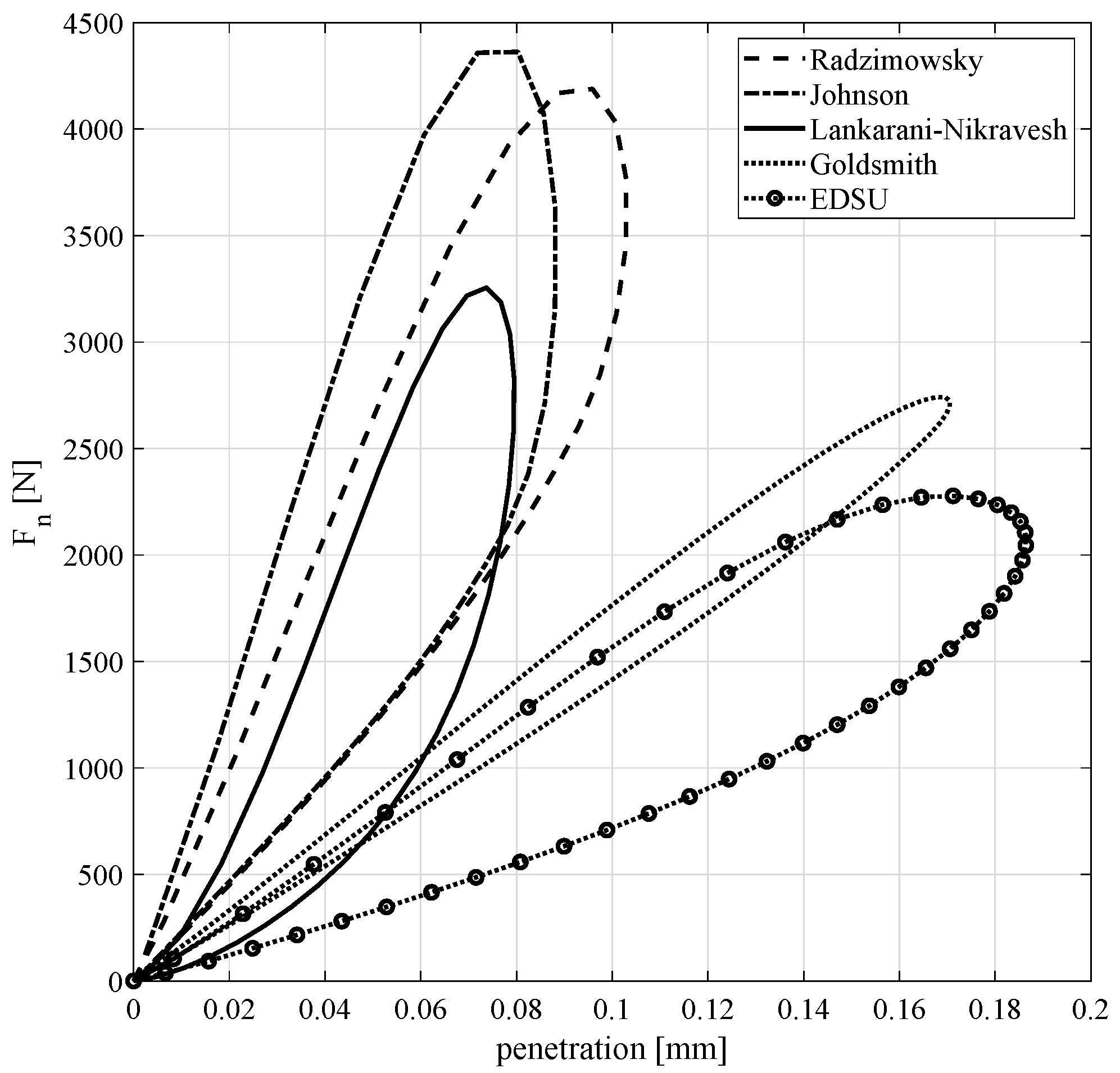
Figure 15 depicts the differences between the hysteresis profile obtained isolating a situation of contact and rebound within the dynamic simulation of interest.

In accordance with the previous considerations, higher forces and more steep loops are noticeable in the Johnson and Radzimowsky models. Conversely, Goldsmith and EDSU exert less abrupt profiles. The Lankarani–Nikravesh model provides intermediate behavior.

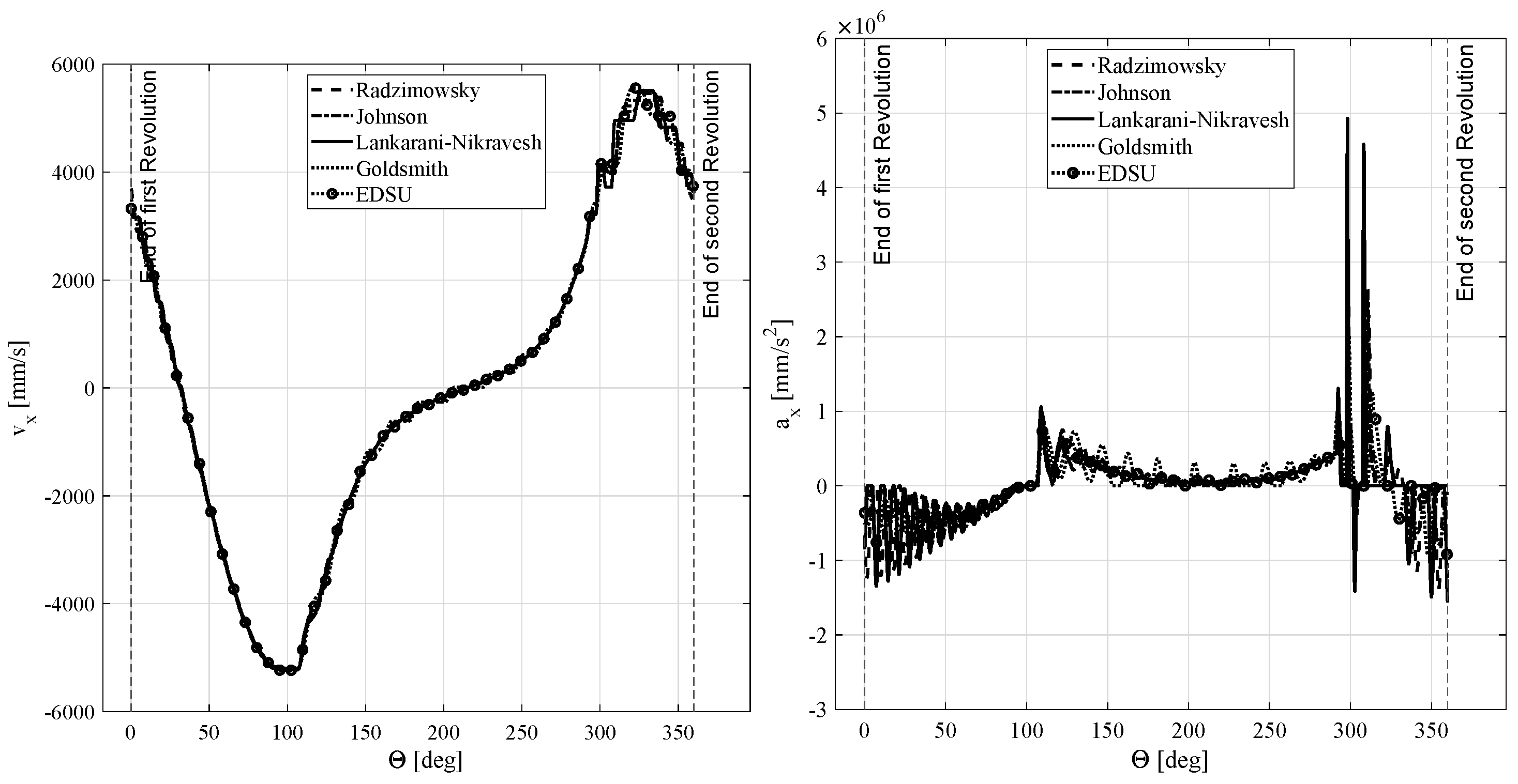
Finally, the contact formulation affects the position, velocity and acceleration of the slider. However, the small clearance between the pin and slot causes the position to be slightly influenced by the contact formulation. Conversely, in the velocity and acceleration plots versus the relative crank angle, some differences are detectable and are consistent with the effects observed in the contact force variation (See Figure 16).

5. Conclusions

The availability of reliable and computationally efficient contact force models is an important requirement in multibody dynamics simulations. A review of methods on the basis of analytical developments and behavior in simulations has been presented herein. Our main focus was the dynamic analysis of mechanisms with the pin-in-the-slot kinematic pairs. The discussion herein offered gives guidelines about the distinctive computational features of each model, but cannot offer a definitive answer on how faithfully the model reproduces reality. This would require an extensive campaign of experimental validation. As an element of novelty and to speed-up the simulation, the polynomial fitting of implicit equations has been presented in tabular form to compute static indentation with different models. Moreover, the possibility of taking into account just one track stiffness instead of differentiating between internal and external contact has been studied. We inferred that this simplification is feasible with small clearances. Lastly, choosing high-stiffness models will provide severe contact forces with high-frequency oscillation, but with a high value of exponent n the contact proved to be more stable in this particular case study.

References

- Pennestri, E.; Stefanelli, R.; Valentini, P.P.; Vita, L. Efficiency and wear in cam actuated robotized gearbox using virtual model. Int. J. Veh. Des. 2008, 46, 347. [Google Scholar] [CrossRef]
- Cera, M.; Cirelli, M.; Pennestrì, E.; Valentini, P. The kinematics of curved profiles mating with a caged idle roller—higher-path curvature analysis. Mech. Mach. Theory 2021, 164, 104414. [Google Scholar] [CrossRef]
- Cera, M.; Cirelli, M.; Pennestrì, E.; Valentini, P.P. Design analysis of torsichrone centrifugal pendulum vibration absorbers. Nonlinear Dyn. 2021, 104, 1023–1041. [Google Scholar] [CrossRef]
- Cirelli, M.; Cera, M.; Pennestrì, E.; Valentini, P.P. Nonlinear design analysis of centrifugal pendulum vibration absorbers: An intrinsic geometry-based framework. Nonlinear Dyn. 2020, 102, 1297–1318. [Google Scholar] [CrossRef]
- Cera, M.; Cirelli, M.; Pennestrì, E.; Valentini, P.P. Nonlinear dynamics of torsichrone CPVA with synchroringed form closure constraint. Nonlinear Dyn. 2021, 105, 2739–2756. [Google Scholar] [CrossRef]
- Cera, M.; Cirelli, M.; Pennestrì, E.; Valentini, P. Design and comparison of centrifugal dampers modern architectures: The influence of roller kinematics on tuning conditions and absorbers nonlinear dynamics. Mech. Mach. Theory 2022, 174, 104876. [Google Scholar] [CrossRef]
- Kobrinsky, A. Mechanisms with Elastic Couplings, NASA Technical Translation TT F-534; Technical Report; NASA: Washington, DC, USA, 1964.
- Lankarani, H.M. Canonical Equations of Motion and Estimation of Parameters in the Analysis of Impact Problems. Ph.D. Thesis, University of Arizona, Tucson, AZ, USA, 1988. [Google Scholar]
- Lankarani, H.M.; Nikravesh, P.E. A contact force model with hysteresis damping for impact analysis of multibody systems. In Proceedings of the 15th Design Automation Conference: Volume 3—Mechanical Systems Analysis, Design and Simulation. American Society of Mechanical Engineers, Montreal, QC, Canada, 17–21 September 1989; pp. 45–51. [Google Scholar] [CrossRef]
- Flores, P.; Ambrósio, J.A.C.; Pimenta Claro, J.C.; Lankarani, H.M. Kinematics and Dynamics of Multibody Systems with Imperfect Joints: Models and Case Studies; Springer International Publishing: Berlin/Heidelberg, Germany, 2010. [Google Scholar]
- Li, W.; Wang, C.; Sheng, C.l.; Yang, H.; Lu, E. Pin-slot clearance joints in multibody systems. Int. J. Precis. Eng. Manuf. 2017, 18, 1719–1729. [Google Scholar] [CrossRef]
- Han, I.; Gilmore, B.J. Multi-Body Impact Motion with Friction Analysis, Simulation, and Experimental Validation. J. Mech. Des. 1993, 115, 412–422. [Google Scholar] [CrossRef]
- Zhang, Y.; Sharf, I. Validation of nonlinear viscoelastic contact force models for low speed impact. J. Appl. Mech. 2009, 76, 051002. [Google Scholar] [CrossRef]
- Flores, P.; Machado, M.; Silva, M.T.; Martins, J.M. On the continuous contact force models for soft materials in multibody dynamics. Multibody Syst. Dyn. 2011, 25, 357–375. [Google Scholar] [CrossRef]
- Keller, J.B. Impact With Friction. J. Appl. Mech. 1986, 53, 1–4. [Google Scholar] [CrossRef]
- Schiehlen, W.; Seifried, R. Three approaches for elastodynamic contact in multibody systems. Multibody Syst. Dyn. 2004, 12, 1–16. [Google Scholar] [CrossRef]
- Gilardi, G.; Sharf, I. Literature survey of contact dynamics modelling. Mech. Mach. Theory 2002, 37, 1213–1239. [Google Scholar] [CrossRef]
- Schwab, A.; Meijaard, J.; Meijers, P. A comparison of revolute joint clearance models in the dynamic analysis of rigid and elastic mechanical systems. Mech. Mach. Theory 2002, 37, 895–913. [Google Scholar] [CrossRef]
- Haddadi, A.; Hashtrudi-Zaad, K. A New Method for Online Parameter Estimation of Hunt-Crossley Environment Dynamic Models. In Proceedings of the 2008 IEEE/RSJ International Conference on Intelligent Robots and Systems, Nice, France, 22–26 September 2008; pp. 981–986. [Google Scholar]
- Zhang, Y. Contact Dynamics for Rigid Bodies: Modeling and Experiments. Ph.D. Thesis, McGill University, Montreal, QC, Canada, 2007. [Google Scholar]
- Pereira, C.M.; Ramalho, A.L.; Ambrósio, J.A.C. A critical overview of internal and external cylinder contact force models. Nonlinear Dyn. 2011, 63, 681–697. [Google Scholar] [CrossRef] [Green Version]
- Machado, M.; Moreira, P.; Flores, P.; Lankarani, H.M. Compliant contact force models in multibody dynamics: Evolution of the Hertz contact theory. Mech. Mach. Theory 2012, 53, 99–121. [Google Scholar] [CrossRef]
- Goldsmith, W. Impact (Dover Civil and Mechanical Engineering), Annotated ed.; Dover Publications: Mineola, NY, USA, 2001; p. 416. [Google Scholar]
- Johnson, K.L. Contact Mechanics, Reprint ed.; Cambridge University Press: Cambridge, UK, 2008; p. 468. [Google Scholar]
- Flores, P.; Lankarani, H.M. Contact force models for multibody dynamics. In Solid Mechanics and Its Applications; Springer International Publishing: Cham, Switzerland, 2016; Volume 226. [Google Scholar] [CrossRef]
- Skrinjar, L.; Slavič, J.; Boltežar, M. A review of continuous contact-force models in multibody dynamics. Int. J. Mech. Sci. 2018, 145, 171–187. [Google Scholar] [CrossRef]
- Koshy, C.S.; Flores, P.; Lankarani, H.M. Study of the effect of contact force model on the dynamic response of mechanical systems with dry clearance joints: Computational and experimental approaches. Nonlinear Dyn. 2013, 73, 325–338. [Google Scholar] [CrossRef]
- Mindlin, R.D. Compliance of elastic bodies in contact. J. Appl. Mech. 1949, 16, 259–268. [Google Scholar] [CrossRef]
- Love, A.E.H. A Treatise on the Mathematical Theory of Elasticity (Dover Books on Engineering), 4th ed.; Dover Publications: Mineola, NY, USA, 2011; p. 672. [Google Scholar]
- Deresiewicz, H. A note on Hertz’s theory of impact. Acta Mech. 1968, 6, 110–112. [Google Scholar] [CrossRef]
- Radzimovsky, E.I. Stress Distribution and Strength Condition of Two Rolling Cylinders Pressed Together; Technical Report; University of Illinois Urbana-Champaign: Champaign, IL, USA, 1953. [Google Scholar]
- Dubowsky, S. The Dynamic Response of Mechanical and Electromechanical Systems with Clearance and Nonlinear Impact Characteristics. Ph.D. Thesis, Columbia University, New York, NY, USA, 1971. [Google Scholar]
- Dubowsky, S.; Freudenstein, F. Dynamic analysis of mechanical systems with clearances Part 1: Formation of dynamic model. J. Eng. Ind. 1971, 93, 305–309. [Google Scholar] [CrossRef]
- Dubowsky, S.; Freudenstein, F. Dynamic analysis of mechanical systems with clearances Part 2: Dynamic response. J. Eng. Ind. 1971, 93, 310–316. [Google Scholar] [CrossRef]
- Lankarani, H.M.; Nikravesh, P.E. A contact force model with hysteresis damping for impact analysis of multibody systems. J. Mech. Des. 1990, 112, 369–376. [Google Scholar] [CrossRef]
- ESDU-78035. Contact Phenomena. I: Stresses, Deflections and Contact Dimensions for Normally-Loaded Unlubricated Elastic Components, Engineering Sciences Data Unit; Technical Report; 1978; ISBN 9780856792397. [Google Scholar]
- Pereira, C.; Ramalho, A.; Ambrósio, J.A.C. Experimental and numerical validation of an enhanced cylindrical contact force model. In Surface Effects and Contact Mechanics X; WIT Transactions on Engineering Sciences; De Hosson, J.M., Brebbia, C., Eds.; WIT Press: Southampton, UK, 2011; Volume 1, pp. 49–60. [Google Scholar] [CrossRef] [Green Version]
- Pereira, C.; Ramalho, A.; Ambrósio, J.A.C. An enhanced cylindrical contact force model. Multibody Syst. Dyn. 2015, 35, 277–298. [Google Scholar] [CrossRef]
- Flores, P.; Ambrósio, J.A.C. Revolute joints with clearance in multibody systems. Comput. Struct. 2004, 82, 1359–1369. [Google Scholar] [CrossRef] [Green Version]
- Flores, P.; Ambrósio, J.A.C.; Pimenta Claro, J.C.; Lankarani, H.M.; Koshy, C.S. A study on dynamics of mechanical systems including joints with clearance and lubrication. Mech. Mach. Theory 2006, 41, 247–261. [Google Scholar] [CrossRef] [Green Version]
- Hunt, K.H.; Crossley, F.R.E. Coefficient of restitution interpreted as damping in vibroimpact. J. Appl. Mech. 1975, 42, 440–445. [Google Scholar] [CrossRef]
- Tatara, Y.; Moriwaki, N. Study on impact of equivalent two bodies: Coefficients of restitution of spheres of brass, lead, glass, porcelain and agate, andthe material properties. Bull. JSME 1982, 25, 631–637. [Google Scholar] [CrossRef] [Green Version]
- Thornton, C. Coefficient of Restitution for Collinear Collisions of Elastic-Perfectly Plastic Spheres. J. Appl. Mech. 1997, 64, 383–386. [Google Scholar] [CrossRef]
- Seifried, R.; Schiehlen, W.; Eberhard, P. Numerical and experimental evaluation of the coefficient of restitution for repeated impacts. Int. J. Impact Eng. 2005, 32, 508–524. [Google Scholar] [CrossRef]
- Minamoto, H.; Kawamura, S. Moderately high speed impact of two identical spheres. Int. J. Impact Eng. 2011, 38, 123–129. [Google Scholar] [CrossRef]
- Herbert, R.G.; McWhannell, D.C. Shape and frequency composition of pulses from an impact pair. J. Eng. Ind. 1977, 99, 513–518. [Google Scholar] [CrossRef]
- Lee, T.W. Optimization of high speed geneva mechanisms. J. Mech. Des. 1981, 103, 621–630. [Google Scholar] [CrossRef]
- Lee, T.W.; Wang, A.C. On The Dynamics of Intermittent-Motion Mechanisms. Part 1: Dynamic Model and Response. J. Mech. Transm. Autom. Des. 1983, 105, 534–540. [Google Scholar] [CrossRef]
- Wang, A.C.; Lee, T.W. On the Dynamics of Intermittent-Motion Mechanisms. Part 2: Geneva Mechanisms, Ratchets, and Escapements. J. Mech. Transm. Autom. Des. 1983, 105, 541–551. [Google Scholar] [CrossRef]
- Wang, A.C. On the Kinematics and Dynamics of Intermittent Motion Mechanisms. Ph.D. Thesis, Rutgers University, New Brunswick, NJ, USA, 1983. [Google Scholar]
- Khulief, Y.A. Dynamic Analysis of Multibody Systems with Intermittent Motion. Ph.D. Thesis, University of Illinois at Chicago, Chicago, IL, USA, 1985. [Google Scholar]
- Khulief, Y.A.; Shabana, A.A. A continuous force model for the impact analysis of flexible multibody systems. Mech. Mach. Theory 1987, 22, 213–224. [Google Scholar] [CrossRef]
- Khulief, Y.A.; Shabana, A.A. Dynamic analysis of constrained system of rigid and flexible bodies with intermittent motion. J. Mech. Transm. Autom. Des. 1986, 108, 38–45. [Google Scholar] [CrossRef]
- Tsuji, Y.; Tanaka, T.; Ishida, T. Lagrangian numerical simulation of plug flow of cohesionless particles in a horizontal pipe. Powder Technol. 1992, 71, 239–250. [Google Scholar] [CrossRef]
- Lankarani, H.M.; Nikravesh, P.E. Continuous contact force models for impact analysis in multibody systems. Nonlinear Dyn. 1994, 5, 193–207. [Google Scholar] [CrossRef]
- Shivaswamy, S. Modeling Contact Forces and Energy Dissipation during Impact in Mechanical Systems. Ph.D. Thesis, Wichita State University, Wichita, KS, USA, 1997. [Google Scholar]
- Shivaswamy, S.; Lankarani, H.M. Impact Analysis of Plates Using Quasi-Static Approach. J. Mech. Des. 1997, 119, 376–381. [Google Scholar] [CrossRef]
- Rhee, J.; Akay, A. Dynamic response of a revolute joint with clearance. Mech. Mach. Theory 1996, 31, 121–134. [Google Scholar] [CrossRef]
- Marhefka, D.; Orin, D. A compliant contact model with nonlinear damping for simulation of robotic systems. IEEE Trans. Syst. Man Cybern. Part A Syst. Hum. 1999, 29, 566–572. [Google Scholar] [CrossRef]
- Gonthier, Y.; McPhee, J.; Lange, C.; Piedœuf, J.C. A Regularized Contact Model with Asymmetric Damping and Dwell-Time Dependent Friction. Multibody Syst. Dyn. 2004, 11, 209–233. [Google Scholar] [CrossRef]
- Machado, M.; Flores, P.; Ambrósio, J.A.C. A Lookup-Table-Based Approach for Spatial Analysis of Contact Problems. J. Comput. Nonlinear Dyn. 2014, 9, 041010. [Google Scholar] [CrossRef] [Green Version]
- Machado, M.; Flores, P.; Pimenta Claro, J.C.; Ambrósio, J.A.C.; Silva, M.; Completo, A.; Lankarani, H.M. Development of a planar multibody model of the human knee joint. Nonlinear Dyn. 2010, 60, 459–478. [Google Scholar] [CrossRef]
- Machado, M.; Flores, P.; Ambrósio, J.A.C. Influence of the contact model on the dynamic response of the human knee joint. Proc. Inst. Mech. Eng. Part K J. Multi-Body Dyn. 2011, 225, 344–358. [Google Scholar] [CrossRef] [Green Version]
- Gharib, M.; Hurmuzlu, Y. A new contact force model for low coefficient of restitution impact. J. Appl. Mech. 2012, 79, 064506. [Google Scholar] [CrossRef]
- Stoianovici, D.; Hurmuzlu, Y. A Critical Study of the Applicability of Rigid-Body Collision Theory. J. Appl. Mech. 1996, 63, 307–316. [Google Scholar] [CrossRef] [Green Version]
- Hu, S.; Guo, X. A dissipative contact force model for impact analysis in multibody dynamics. Multibody Syst. Dyn. 2015, 35, 131–151. [Google Scholar] [CrossRef]
Figure 2.
Hunt and Crossley: Indentation force hysteresis loop [41], where the area of such a loop represents the energy loss.
Figure 3.
Transition function [48].
Figure 5.
Indentation versus time for a Hertz-type contact force model [35].
Figure 6.
The relationship between and the coefficient of restitution e [54].
Figure 7.
Contact force model with permanent indentation. (a) contact force versus time, (b) indentation versus time [55].
Figure 8.
Scotch-yoke linkage.
Figure 9.
Scotch-yoke linkage, without (left) and with clearance (right).
Figure 10.
Effect of clearance on the error.
Figure 11.
Contact force comparison.
Figure 12.
Penetration comparison.
Figure 13.
Detail of penetration comparison.
Figure 14.
Detail of contact force comparison.
Figure 15.
Hysteresis comparison.
Figure 16.
Slotted slider kinematics.