Statistical Evaluations and Applications for IER Parameters from Generalized Progressively Type-II Hybrid Censored Data

Abstract

Generalized progressively Type-II hybrid strategy has been suggested to save both the duration and cost of a life test when the experimenter aims to score a fixed number of failed units. In this paper, using this mechanism, the maximum likelihood and Bayes inferential problems for unknown model parameters, in addition to both reliability, and hazard functions of the inverted exponentiated Rayleigh model, are acquired. Applying the observed Fisher data and delta method, the normality characteristic of the classical estimates is taken into account to derive confidence intervals for unknown parameters and several indice functions. In Bayes’ viewpoint, through independent gamma priors against both symmetrical and asymmetrical loss functions, the Bayes estimators of the unknown quantities are developed. Because the Bayes estimators are acquired in complicated forms, a hybrid Monte-Carlo Markov-chain technique is offered to carry out the Bayes estimates as well as to create the related highest posterior density interval estimates. The precise behavior of the suggested estimation approaches is assessed using wide Monte Carlo simulation experiments. Two actual applications based on actual data sets from the mechanical and chemical domains are examined to show how the offered methodologies may be used in real current events.

1. Introduction

In reliability experiments or clinical trials, the failure times of experimental objects are frequently unavailable. Censoring strategies are commonly used to save money while also limiting the amount of time spent on experiments. The two most popular censorship mechanisms, called; Type-I (or time) and Type-II (or failure) censoring strategies. These plans have been studied in detail by Bain and Engelhardt [1]. Two mixtures of Type-I and Type-II techniques, called hybrid Type-I hybrid (T1H) and Type-II hybrid (T2H), are introduced by Epstein [2] and Childs et al. [3], respectively. Although a vast amount of literature is available on the given schemes, they do not allow for the withdrawal of live test items at other times than when the test ends. So, these plans do not have the flexibility to allow subjects to be removed, and they will not be beneficial to use. Therefore, to overcome this drawback, Type-I and Type-II progressive as well as Type-I progressive hybrid (T1PH) and Type-II progressive hybrid (T2PH) censored mechanisms are discussed in detail by an excellent monograph presented by Balakrishnan and Cramer [4]. Unfortunately, although T2PH has become very common in reliability tests, it can take a long duration to stop the test, and thus inference procedures may be unworkable or ineffective. To address the disadvantages, Ng et al. [5] proposed adaptive-T2PH to benefit from reducing the total test duration and enhancing grading efficiency.

Despite both T2PH and adaptive-T2PH censoring strategies ensure a certain amount of failures, their disadvantage is that it may take quite some time to detect the required m failures and end the test. As a result, Lee et al. [6] proposed a generalized-T2PH technique in which the study is certain to stop at a fixed time. They stated that the study carried out based on the generalized-T2PH plan could save overall time on testing and cost. We briefly explain this strategy as: Suppose n subjects are put on an experiment at time 0, the size of censored sample $m(<n)$, the progressive design $\mathbf{R}=(R_1,\cdots ,R_m)$ and $T_i,i=1,2,$ (where $0<T_1<T_2<\infty$) must be prefixed. Let ($d_1,d_2$) be the length of the observed failures before ($T_1,T_2$). However, as soon as the first failure (say $y_{1:m:n}$) occurs, $R_1$ (of $n-1$) are randomly drawn from the experiment; next when second failure (say $y_{2:m:n}$) occurs, $R_2$ (of $n-1-R_1$) are randomly drawn, and so on. Then, at time ${\mathcal{T}}^{•}=\max \left\{T_1,\min \left\{Y_{m:m:n},T_2\right\}\right\}$, the testing stopped. Clearly, $T_2$ represents the greatest time for which the researcher is ready to continue the examination.

The main feature of this process is that it might occur when the participant has planned to use the testing facility for two time limitations by changing the values of some of the progressive units during the experiment. However, if $Y_{m:m:n}<T_1$, end the test at $T_1$ (Case-I); If $T_1<Y_{m:m:n}<T_2$, end the test at $Y_{m:m:n}$ (Case-II); otherwise, stop the test at $T_2$ (Case-III). Practically, the experimenter collects one of the following data groups:

$$\{\mathbf{Y},\mathbf{R}\}=\left\{\begin{array}{cccc}\hfill & \{(Y_{1:m:n},R_1),\cdots ,(Y_{m-1:m:n},R_{m-1}),(Y_{m:m:n},0),\cdots ,(Y_{d_1:n},0)\};\hfill & & \mathrm{Case-I},\\ \hfill & \{(Y_{1:m:n},R_1),\cdots ,(Y_{d_1:n},R_{d_1}),\cdots ,(Y_{m-1:m:n},R_{m-1}),(Y_{m:m:n},R_m)\};\hfill & & \hspace{0.17em}\mathrm{Case-II},\\ \hfill & \{(Y_{1:m:n},R_1),\cdots ,(Y_{d_1:n},R_{d_1}),\cdots ,(Y_{d_2-1:n},R_{d_2-1}),(Y_{d_2:n},R_{d_2})\};\hfill & & \hspace{0.17em}\mathrm{Case-III}.\end{array}\right.$$

Let $\{\mathbf{Y},\mathbf{R}\}$ represent order statistics collected from a generalized-T2PH censoring, which come from a continuous population with probability density function (PDF) (symbolized by $f(·)$) and cumulative distribution function (CDF) (symbolized by $F(·)$). Then, the joint PDF of $\{\mathbf{Y},\mathbf{R}\}$ can be expressed as

$${\mathcal{L}}_{\xi }\left(\omega \right|\mathbf{Y})=G_{\xi }{\mathrm{\Psi }}_{\xi }(T_{\tau };\omega ){\prod }_{i=1}^{D_{\xi }}f(y_{i:m:n};\omega ){\left[1-F(y_{i:m:n};\omega )\right]}^{R_i},\xi =1,2,3,\tau =1,2,$$

(1)

where $\omega$ is a vector of interested parameters.

Table 1. Notations of the generalized-T2PH censoring.

$\mathit{\xi }$	${\mathit{G}}_{\mathit{\xi }}$	${\mathit{D}}_{\mathit{\xi }}$	${\mathbf{\Psi }}_{\mathit{\xi }}({\mathit{T}}_{\mathit{\tau }};\mathit{\omega })$	${\mathit{R}}_{{\mathit{d}}_{\mathit{\tau }}+1}^{*}$
1	${\mathrm{\Pi }}_{i=1}^{d_1}{\sum }_{r=i}^m\left(R_r+1\right)$	$d_1$	${\left[1-F\left(T_1\right)\right]}^{R_{d_1+1}^{*}}$	$n-{\sum }_{r=1}^{m-1}{R}_{rr}-d_1$
2	${\mathrm{\Pi }}_{i=1}^m{\sum }_{r=i}^m\left(R_r+1\right)$	m	1	0
3	${\mathrm{\Pi }}_{i=1}^{d_2}{\sum }_{r=i}^m\left(R_r+1\right)$	$d_2$	${\left[1-F\left(T_2\right)\right]}^{R_{d_2+1}^{*}}$	$n-{\sum }_{r=1}^{d_2}{R}_r-d_2$

provides the notations $\xi$, $G_{\xi }$, $D_{\xi }$, ${\mathrm{\Psi }}_{\xi }(T_{\tau };\omega )$ and $R_{d_{\tau }+1}^{*}$ of the generalized-T2PH censoring. Further, from (1), various censoring techniques are reported in Table 2. Several research investigations have been conducted on the statistical estimate of unknown parameter(s) and/or reliability indices in various lifespan models using generalized-T2PH data; e.g., see Ashour and Elshahhat [7], Ateya and Mohammed [8], Seo [9], Cho and Lee [10], Nagy et al. [11], Wang et al. [12], Elshahhat et al. [13], later Alotaibi et al. [14], among others.

The Rayleigh model is a particular kind of the Weibull lifetime model, which was initially suggested by Rayleigh while researching acoustics difficulties. Because it just has one parameter, its practical uses are restricted and un-flexible. Therefore, Ghitany et al. [15] proposed a novel general group of inverse exponentiated distributions in which the two-parameter inverted exponentiated Rayleigh (IER) distribution is a particular member and its failure rate is non-monotonic if the failure rates of testing elements are not monotonous and show a pattern of change. However, suppose Y is a nonnegative random variable of a test item that follows the IER distribution, denoted by $\mathrm{IER}\left(\omega \right)$, where $\omega ={(\delta ,\mu )}^{\mathsf{T}}$, $\delta >0$ is the shape and $\mu >0$ is the scale parameters, respectively. Thus, its PDF, CDF, and hazard rate function (HRF), (symbolized by $h(·)$), are given respectively by

$$\begin{array}{cccc}\hfill f(y;\omega )& =2\delta \mu y^{-3}{e}^{-\mu y^{-2}}{\left(1-e^{-\mu y^{-2}}\right)}^{\delta -1},\hfill & \hfill & y>0;\hfill \end{array}$$

(2)

$$\begin{array}{cccc}\hfill F(y;\omega )& =1-{\left(1-e^{-\mu y^{-2}}\right)}^{\delta },\hfill & \hfill & y>0;\hfill \end{array}$$

(3)

$$\begin{array}{cccc}\hfill h(t;\omega )& =2\delta \mu t^{-3}{e}^{-\mu t^{-2}}{\left(1-e^{-\mu t^{-2}}\right)}^{-1},\hfill & \hfill & t>0;\hfill \end{array}$$

(4)

and its reliability (or survival) function (RF) given by $R(·)=1-F(·)$.

In literature, using different sampling scenarios, several authors have done significant work on the theories and applications of the IER model, for example, Rastogi and Tripathi [16] analyzed hybrid Type-I; independently, Kayal et al. [17] as well as Maurya et al. [18] analyzed progressive Type-II; independently, Gao and Gui [19] as well as Maurya et al. [20] analyzed progressive first-failure; Gao and Gui [21] discussed the pivotal inference from progressive Type-II; Panahi and Moradi [22] analyzed an adaptive Type II progressive hybrid; recently Fan and Gui [23] analyzed joint progressively Type-II censoring mechanisms.

Table 2. Six special cases from generalized-T2PH censoring.

Plan	Author(s)	Setting
T1PH	Kundu and Joarder [24]	$T_1\to 0$
T2PH	Childs et al. [25]	$T_2\to \infty$
T1H	Epstein [2]	$T_1\to 0$, $R_i=0,i=1,2,\cdots ,m-1,$ and $R_m=n-m$
T2H	Childs et al. [3]	$T_2\to \infty$, $R_i=0,i=1,2,\cdots ,m-1,$ and $R_m=n-m$
Type-I	Bain and Engelhardt [1]	$T_1=0$, $m=n$, $R_i=0,i=1,2,\cdots ,m-1,$ and $R_m=n-m$
Type-II	Bain and Engelhardt [1]	$T_1=0$, $T_2\to \infty$, $R_i=0,i=1,2,\cdots ,m-1,$ and $R_m=n-m$

Table 2. Six special cases from generalized-T2PH censoring.

Plan	Author(s)	Setting
T1PH	Kundu and Joarder [24]	$T_1\to 0$
T2PH	Childs et al. [25]	$T_2\to \infty$
T1H	Epstein [2]	$T_1\to 0$, $R_i=0,i=1,2,\cdots ,m-1,$ and $R_m=n-m$
T2H	Childs et al. [3]	$T_2\to \infty$, $R_i=0,i=1,2,\cdots ,m-1,$ and $R_m=n-m$
Type-I	Bain and Engelhardt [1]	$T_1=0$, $m=n$, $R_i=0,i=1,2,\cdots ,m-1,$ and $R_m=n-m$
Type-II	Bain and Engelhardt [1]	$T_1=0$, $T_2\to \infty$, $R_i=0,i=1,2,\cdots ,m-1,$ and $R_m=n-m$

Although a great deal of work has been done on the IER lifetime model, to the best of our experience, no effort has been achieved to discuss the IER’s model parameters and(or) reliability time features when the sample is a generalized-T2PH censored strategy. To fill up this issue, using the proposed censoring plan, the main contribution of the present study is three-fold:

• Maximum likelihood estimators (MLEs) along with their approximate confidence intervals (ACIs) of $\delta$, $\mu$, $R\left(t\right)$ and $h\left(t\right)$ are obtained.
• Bayes’ estimators under independent gamma assumptions of $\delta$, $\mu$, $R\left(t\right)$ and $h\left(t\right)$ are created relative to the squared-error (SE) and general-entropy (GE) losses.
• Bayes estimators cannot be estimated in explicit form, so Markov-chain Monte-Carlo (MCMC) approximation techniques are recommended to compute the acquired Bayes MCMC estimates and the associated highest posterior density (HPD) intervals.
• Numerical solutions for the offered estimators of $\delta$, $\mu$, $R\left(t\right)$ and $h\left(t\right)$ are done by installing two useful packages, namely: ‘$\mathsf{coda}$’ (proposed by Plummer et al. [26]) and ‘$\mathsf{maxLik}$’ (proposed by Henningsen and Toomet [27]) on the $\mathsf{R}$ 4.2.2 programming platform.
• Extensive Monte Carlo comparisons, on the basis of four accuracy criteria, namely: (i) root mean squared-errors; (ii) mean relative absolute-biases; (iii) average confidence lengths; and (iv) coverage percentages, the behavior of the acquired estimators of $\delta$, $\mu$, $R\left(t\right)$ and $h\left(t\right)$ is discussed.
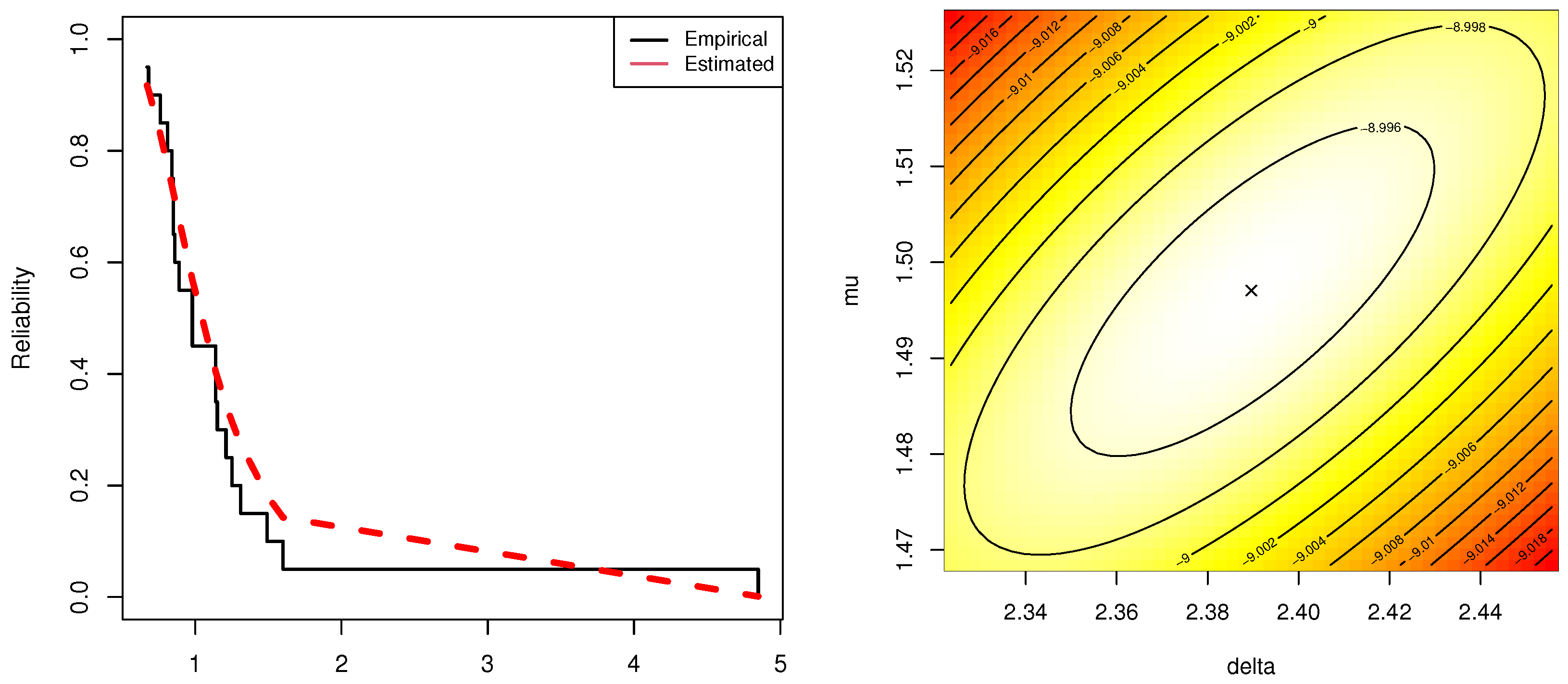
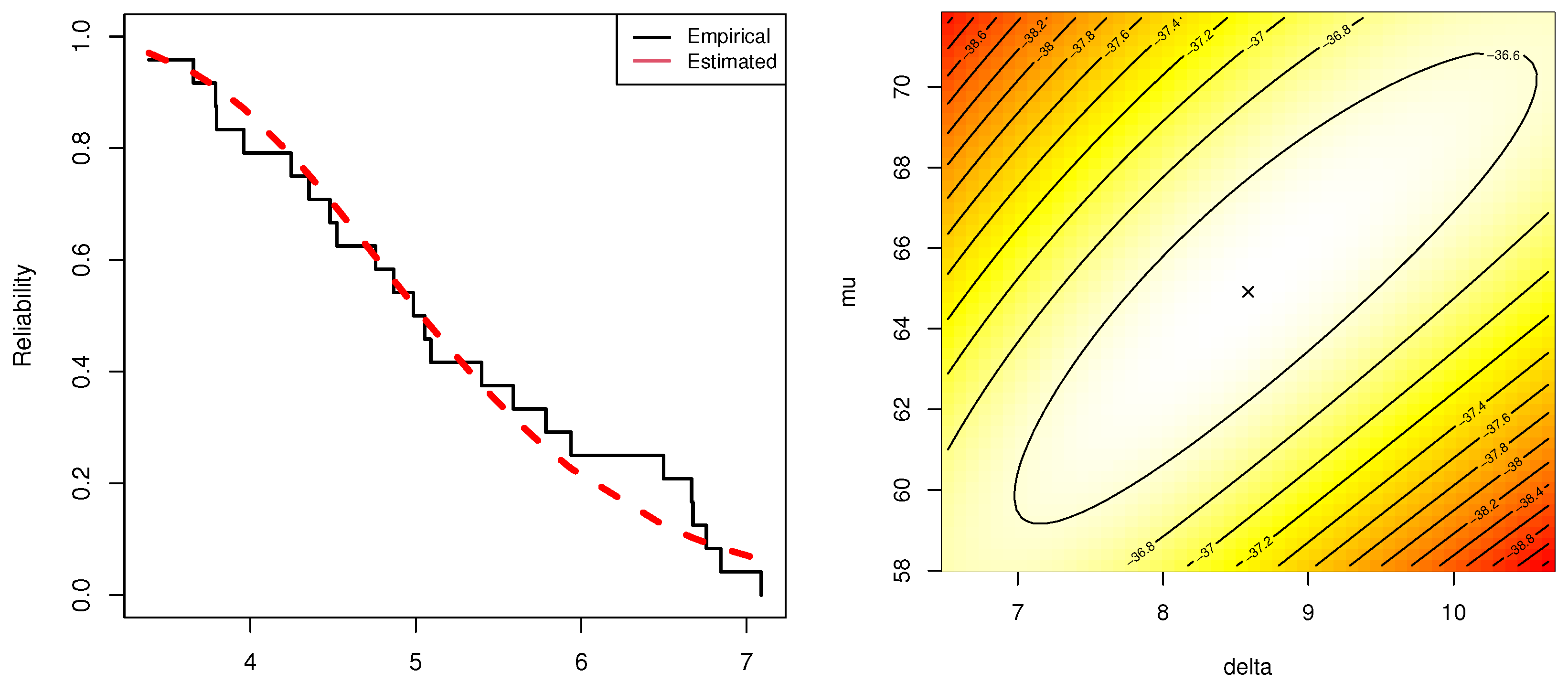
• To benefit from the practicality and flexibility of the IER model in data analysis, from the engineering and chemistry areas, we analyzed different real data sets that reflect failure times of mechanical components and cumin essential oil.

The rest of the work is classified as follows: Section 2 investigates both maximum likelihood and Bayesian inferences. Monte Carlo simulations are reported in Section 3. In Section 4, two real applications are explored. Lastly, Section 5 provides some concluding remarks and recommendations of the study.

2. Inferences

In this section, based on generalized-T2PH censored data, we have obtained the maximum likelihood and Bayes’ estimators as well as their ACI/HPD interval estimators of $\delta$, $\mu$, $R\left(t\right)$ and $h\left(t\right)$.

2.1. Likelihood Estimation

Let $\mathbf{y}=\{y_{i:m:n},R_i\}$ be a generalized-T2PH censored data of size $d_2$ obtained from the $\mathrm{IER}(\delta ,\mu )$ population with PDF and CDF in (2) and (3), respectively. Using (2), (3) and (1), such $y_i$ is a simplicity notation of $y_{i:m:n}$, we can express (1) up to proportional as

$${\mathcal{L}}_{\xi }\left(\omega \right|\mathbf{y})\propto {\mathrm{\Psi }}_{\xi }\left(T_{\tau };\omega \right){\left(\delta \mu \right)}^{D_{\xi }}{e}^{-\mu {\sum }_{i=1}^{D_{\xi }}{y}_i^{-2}}\prod _{i=1}^{D_{\xi }}{\left(1-e^{-\mu y_i^{-2}}\right)}^{\delta \left(R_i+1\right)-1},$$

(5)

where

${\mathrm{\Psi }}_1\left(T_1;\omega \right)={\left(1-e^{-\mu T_1^{-2}}\right)}^{\delta R_{d_1+1}^{*}}$, ${\mathrm{\Psi }}_2\left(T_{\tau };\omega \right)=1$ and ${\mathrm{\Psi }}_3\left(T_2;\omega \right)={\left(1-e^{-\mu T_2^{-2}}\right)}^{\delta R_{d_2+1}^{*}}$.

Correspondingly, the log-likelihood function, ${\mathsf{\ell }}_{\xi }(·)\propto \log {\mathcal{L}}_{\xi }(·)$, becomes

$$\mathsf{\ell }\left(\omega |\mathbf{y}\right)\propto {\mathrm{{\rm Y}}}_{\xi }\left(T_{\tau };\omega \right)+D_{\xi }\log \left(\delta \mu \right)-\mu \sum _{i=1}^{D_{\xi }}{y}_i^{-2}+\sum _{i=1}^{D_{\xi }}\left(\delta \left(R_i+1\right)-1\right)\log \left(1-e^{-\mu y_i^{-2}}\right),$$

(6)

where ${\mathrm{{\rm Y}}}_{\xi }\left(T_{\tau };\omega \right)=\log {\mathrm{\Psi }}_{\xi }\left(T_{\tau };\omega \right)$ for $\xi =1,2,3,$ and $\tau =1,2$.

Differentiating (6) with regard to $\delta$ and $\mu$, to obtain the MLEs $\widehat{\delta }$ and $\widehat{\mu }$, respectively, we get

$$\frac{\partial \mathsf{\ell }}{\partial \delta }={\mathrm{{\rm Y}}}_{\xi }^{\circ }\left(T_{\tau };\omega \right)+D_{\xi }{\delta }^{-1}+\sum _{i=1}^{D_{\xi }}\left(R_i+1\right)\log \left(1-e^{-\mu y_i^{-2}}\right),$$

(7)

and

$$\frac{\partial \mathsf{\ell }}{\partial \mu }={\mathrm{{\rm Y}}}_{\xi }^{•}\left(T_{\tau };\omega \right)+D_{\xi }{\mu }^{-1}+\sum _{i=1}^{D_{\xi }}\left(\delta \left(R_i+1\right)-1\right)y_i^{-2}{e}^{-\mu y_i^{-2}}{\left(1-e^{-\mu y_i^{-2}}\right)}^{-1},$$

(8)

where

${\mathrm{{\rm Y}}}_{\xi }^{\circ }\left(T_{\tau };\omega \right)=R_{d_{\tau }+1}^{*}\log \left(1-e^{-\mu T_{\tau }^{-2}}\right)$ and ${\mathrm{{\rm Y}}}_{\xi }^{•}\left(T_{\tau };\omega \right)=\delta R_{d_{\tau }+1}^{*}{T}_{\tau }^{-2}{e}^{-\mu T_{\tau }^{-2}}{\left(1-e^{-\mu T_{\tau }^{-2}}\right)}^{-1}$.

It is obvious, from (7) and (8), that the MLEs $\widehat{\delta }$ and $\widehat{\mu }$ of $\delta$ and $\mu$, respectively, are expressed in nonlinear formulas. So, we recommend to utilize the Newton-Raphson technique by ‘$\mathsf{maxLik}$’ (suggested by Henningsen and Toomet [27]) to acquire the desired estimators $\widehat{\delta }$ and $\widehat{\mu }$.

To prove the existence and uniqueness of $\widehat{\delta }$ and $\widehat{\mu }$, using one simulated generalized-T2PH censored sample when $(\delta ,\mu )=(0.5,1)$, $(T_1,T_2)=(0.5,1.5)$, $(n,m)=(80,40)$ and $R_i=1,i=1,\cdots ,m$, the profile log-likelihood plots of $\delta$ and $\mu$ are shown in Figure 1. In this situation, the MLE values of $\delta$ and $\mu$ are 0.61525 and 1.52502, respectively. Figure 1 provides evidence that the acquired MLEs $\widehat{\delta }$ and $\widehat{\mu }$ of $\delta$ and $\mu$ existed and were unique.

Once the estimates of $\widehat{\delta }$ and $\widehat{\mu }$ evaluated, the MLEs $\widehat{R}\left(t\right)$ and $\widehat{h}\left(t\right)$ of $R\left(t\right)$ and $h\left(t\right)$, are given (for $t>0$) respectively by

$$\widehat{R}\left(t\right)={\left(1-e^{-\widehat{\mu }{t}^{-2}}\right)}^{\widehat{\delta }}\mathrm{and}\widehat{h}\left(t\right)=2\widehat{\delta }\widehat{\mu }{t}^{-3}{e}^{-\widehat{\mu }{t}^{-2}}{\left(1-e^{-\widehat{\mu }{t}^{-2}}\right)}^{-1}.$$

Now, using the asymptotic normality of $\widehat{\delta }$ and $\widehat{\mu }$, the associated ACI of $\delta$, $\mu$, $R\left(t\right)$ or $h\left(t\right)$ is constructed, see Lawless [28]. It is clear, according to the theory of large-sample, that the asymptotic distribution of $\widehat{\delta }$ and $\widehat{\mu }$ (say $\widehat{\omega }={(\widehat{\delta },\widehat{\mu })}^{\top }$) is normal distribution with mean $\omega$ and variance ${\mathbf{I}}^{-1}\left(\omega \right)$.

Through inverting the observed Fisher’s information matrix, the estimated asymptotic variance–covariance ${\mathbf{I}}^{-1}\left(\omega \right)$ matrix can be offered via replacing ($\delta ,\mu$) with ($\widehat{\delta },\widehat{\mu }$) as

$${\mathbf{I}}^{-1}\left(\widehat{\omega }\right)\cong {\left[\begin{array}{c}-{\mathcal{L}}_{11}-{\mathcal{L}}_{12}\\ -{\mathcal{L}}_{21}-{\mathcal{L}}_{22}\end{array}\right]}_{}^{-1}=\left[\begin{array}{c}{\widehat{\sigma }}_{11}{\widehat{\sigma }}_{12}\\ {\widehat{\sigma }}_{21}{\widehat{\sigma }}_{22}\end{array}\right],$$

(9)

where

$${\mathcal{L}}_{11}={\mathrm{{\rm Y}}}_{\xi }^{\circ \circ }\left(T_{\tau };\omega \right)-D_{\xi }{\delta }^{-2},$$

$$\begin{array}{cc}\hfill {\mathcal{L}}_{22}& ={\mathrm{{\rm Y}}}_{\xi }^{••}\left(T_{\tau };\omega \right)-D_{\xi }{\mu }^{-2}\hfill \\ \hfill & -{\sum }_{i=1}^{D_{\xi }}\left(\delta \left(R_i+1\right)-1\right)y_i^{-4}{e}^{-\mu y_i^{-2}}{\left(1-e^{-\mu y_i^{-2}}\right)}^{-1}\left[1+e^{-\mu y_i^{-2}}{\left(1-e^{-\mu y_i^{-2}}\right)}^{-1}\right],\hfill \end{array}$$

and

$${\mathcal{L}}_{12}={\mathrm{{\rm Y}}}_{\xi }^{\circ •}\left(T_{\tau };\omega \right)+{\sum }_{i=1}^{D_{\xi }}\left(R_i+1\right)y_i^{-2}{e}^{-\mu y_i^{-2}}{\left(1-e^{-\mu y_i^{-2}}\right)}^{-1},$$

with

$${\mathrm{{\rm Y}}}_{\xi }^{\circ \circ }\left(T_{\tau };\omega \right)=0,$$

$${\mathrm{{\rm Y}}}_{\xi }^{••}\left(T_{\tau };\omega \right)=-\delta R_{d_{\tau }+1}^{*}{T}_{\tau }^{-4}{e}^{-\mu T_{\tau }^{-2}}{\left(1-e^{-\mu T_{\tau }^{-2}}\right)}^{-1}\left[1+e^{-\mu T_{\tau }^{-2}}{\left(1-e^{-\mu T_{\tau }^{-2}}\right)}^{-1}\right],$$

and

$${\mathrm{{\rm Y}}}_{\xi }^{\circ •}\left(T_{\tau };\omega \right)=R_{d_{\tau }+1}^{*}{T}_{\tau }^{-2}{e}^{-\mu T_{\tau }^{-2}}{\left(1-e^{-\mu T_{\tau }^{-2}}\right)}^{-1}.$$

Thus, the $100(1-q)\%$ ACI bounds for $\delta$ and $\mu$ are given by

$$\widehat{\delta }\mp z_{q/2}\sqrt{{\widehat{\sigma }}_{11}}\mathrm{and}\widehat{\mu }\mp z_{q/2}\sqrt{{\widehat{\sigma }}_{22}},$$

respectively, where $z_{q/2}$ is the $(q/2)$th standard normal variate.

Furthermore, to build the ACI of $R\left(t\right)$ or $h\left(t\right)$, the delta method is considered to approximate the estimated variance associated with the MLEs $\widehat{R}\left(t\right)$ or $\widehat{h}\left(t\right)$, denoted by ${\widehat{\sigma }}_R$ and ${\widehat{\sigma }}_h$, as

$${\widehat{\sigma }}_R={\left.{\mathcal{A}}_R^{\mathsf{T}}{\mathbf{I}}^{-1}\left(\vartheta \right){\mathcal{A}}_R\right|}_{(\widehat{\delta },\widehat{\mu })}\mathrm{and}{\widehat{\sigma }}_h={\left.{\mathcal{A}}_h^{\mathsf{T}}{\mathbf{I}}^{-1}\left(\vartheta \right){\mathcal{A}}_h\right|}_{(\widehat{\delta },\widehat{\mu })}$$

respectively, where ${\mathcal{A}}_R^{\mathsf{T}}=\left[\frac{\partial R\left(t\right)}{\partial \delta }\frac{\partial R\left(t\right)}{\partial \mu }\right]$ and ${\mathcal{A}}_h^{\mathsf{T}}=\left[\frac{\partial h\left(t\right)}{\partial \delta }\frac{\partial h\left(t\right)}{\partial \mu }\right]$.

So, the $100(1-q)\%$ ACI bounds of $R\left(t\right)$ and $h\left(t\right)$ are

$$\left(\widehat{R}\left(t\right)\mp z_{q/2}\sqrt{{\widehat{\sigma }}_R}\right)\mathrm{and}\left(\widehat{h}\left(t\right)\mp z_{q/2}\sqrt{{\widehat{\sigma }}_h}\right),$$

respectively.

2.2. Bayes Estimation

This subsection considers the Bayes approach to estimate the parameters $\delta$ and $\mu$, reliability $R\left(t\right)$ and hazard $h\left(t\right)$ functions of the IER model when a data set from the generalized-T2PH censored collected. To establish this objective, the gamma $G(·)$ density priors are utilized to adapt support of IER parameters. So, both $\delta$ and $\mu$ are considered to be independent stochastically with gamma priors distributed such as $\delta \sim G(a_1,b_1)$ and $\mu \sim G(a_2,b_2)$. Then, for $a_i,b_i>0,i=1,2$, the joint prior PDF (say $\varphi (·)$) of $\delta$ and $\mu$ is

$$\varphi \left(\delta ,\mu \right)\propto {\delta }^{a_1-1}{\mu }^{a_2-1}{e}^{-\left(b_1\delta +b_2\mu \right)},\delta ,\mu >0,$$

(10)

where $a_i$ and $b_i$ are supposed to be known.

Combining (5) with (10), the joint posterior PDF (say $\mathrm{\Sigma }(·)$) of $\delta$ and $\mu$ becomes

$$\begin{array}{c}\hfill {\mathrm{\Sigma }}_{\xi }\left(\omega \right|\mathbf{y})\propto {\mathrm{\Psi }}_{\xi }\left(T_{\tau };\omega \right){\delta }^{D_{\xi }+a_1-1}{\mu }^{D_{\xi }+a_2-1}{e}^{-\left(\delta b_1+\mu \left(b_2+{\sum }_{i=1}^{D_{\xi }}{y}_i^{-2}\right)\right)}\prod _{i=1}^{D_{\xi }}{\left(1-e^{-\mu y_i^{-2}}\right)}^{\delta \left(R_i+1\right)-1},\end{array}$$

(11)

where its normalized term (say $\mathcal{H}$) is given by $\mathcal{H}={\int }_0^{\infty }{\int }_0^{\infty }{\mathrm{\Sigma }}_{\xi }\left(\omega \right|\mathbf{y})\mathrm{d}\delta \mathrm{d}\mu .$

In Bayes’ methodology, a loss function is important in Bayesian estimation because it may detect overestimating and underestimating in the research. Here, two commonly employed symmetric and asymmetric loss functions, namely: SE (symmetric) and GE (asymmetric) loss functions, are considered. However, under the SE loss, the Bayes estimator is provided simply by the posterior mean, where overestimation and underestimation are addressed equally. In practice, however, this may not make sense. Keeping this in mind, a variety of asymmetric loss functions are proposed in the statistical literature. So, we shall use the GE loss function, which provides varying degrees of relevance for overestimation and underestimation, for additional details, see Calabria and Pulcini [29]. Now, let $\zeta (\delta ,\mu )$ be an unknown parametric function of $\delta$ and $\mu$, then the desired Bayes estimators against the SE (say ${\tilde{\zeta }}_S(·)$) and GE (${\tilde{\zeta }}_G(·)$) loss are given by

$$\begin{array}{c}\hfill {\tilde{\zeta }}_S(\delta ,\mu )={\int }_0^{\infty }{\int }_0^{\infty }\zeta (\delta ,\mu )g(\delta ,\mu |\mathbf{y})\mathrm{d}\delta \mathrm{d},\end{array}$$

(12)

and

$$\begin{array}{c}\hfill {\tilde{\zeta }}_G(\delta ,\mu )={\left[{\int }_0^{\infty }{\int }_0^{\infty }{\left[\zeta (\delta ,\mu )\right]}^{-\nu }g(\delta ,\mu |\mathbf{y})\mathrm{d}\delta \mathrm{d}\mu \right]}^{-\frac{1}{\nu }},\end{array}$$

(13)

respectively, when $\nu \to -1$, the Bayes estimate derived from SE loss will be the same as the Bayes estimate derived from GE loss. It is preferable to note that other types of loss from symmetric or asymmetric families can be easily incorporated.

Clearly, using (12) and (13), the Bayes estimators ${\tilde{\zeta }}_S(\delta ,\mu )$ and ${\tilde{\zeta }}_G(\delta ,\mu )$ cannot be derived analytically. As a result, we suggest performing the MCMC techniques to evaluate the offered Bayes estimates of $\delta$, $\mu$, $R\left(t\right)$ and $h\left(t\right)$.

Before going to build the MCMC steps, the full distributions of $\delta$ and $\mu$ must first be derived as

$$\begin{array}{c}\hfill K_1\left(\left.\delta \right|\mathbf{y},\mu \right)\propto {\delta }^{D_{\xi }+a_1-1}{e}^{-\delta \vartheta \left(\left.\omega \right|\mathbf{y}\right)},\end{array}$$

(14)

and

$$\begin{array}{c}\hfill K_2\left(\left.\mu \right|\mathbf{y},\delta \right)\propto {\mu }^{D_{\xi }+a_2-1}{e}^{-\mu \left(b_2-{\mathrm{{\rm Y}}}_{\xi }\left(T_{\tau };\omega \right)+{\sum }_{i=1}^{D_{\xi }}{y}_i^{-2}\right)}\prod _{i=1}^{D_{\xi }}{\left(1-e^{-\mu y_i^{-2}}\right)}^{\delta \left(R_i+1\right)-1},\end{array}$$

(15)

respectively, where $\vartheta \left(\left.\omega \right|\mathbf{y}\right)=b_1-{\delta }^{-1}{\mathrm{{\rm Y}}}_{\xi }\left(T_{\tau };\omega \right)-{\sum }_{i=1}^{D_{\xi }}\left(R_i+1\right)\log \left(1-e^{-\mu y_i^{-2}}\right).$

It is noted, from (14) and (15), that the shape parameter $\delta$ follows the gamma distribution with shape parameter $(D_{\xi }+a_1)$ and scale parameter $\vartheta \left(\left.\omega \right|\mathbf{y}\right)$, therefore any gamma-generating operator can be easily utilized to simulate samples of $\delta$. On the other hand, it is impossible to reduce the conditional distribution (15) of $\mu$ to any known statistical model. So, we employ the Metropolis–Hasting (to update $\mu$) within the Gibbs sampler (to update $\delta$) to adopt the MCMC samples of $\delta$ and $\mu$. In practice, it can be difficult to find starting points near the posterior mode, and due to the fact that the initial values do not affect the parameter estimates, given a sufficiently long chain, we recommend the MLEs as good starting points for running the proposed MCMC algorithm, see Van Ravenzwaaij et al. [30]. However, to acquire the Bayes’ estimates and to create their HPD interval bounds of $\delta$, $\mu$, $R\left(t\right)$ and $h\left(t\right)$, do:

Step 1: 

Set the initial guesses $({\delta }^{\left(0\right)},{\mu }^{\left(0\right)})=(\widehat{\delta },\widehat{\mu })$.

Step 2: 

Set $ϵ=1$.

Step 3: 

Generate ${\delta }^{\left(\right)}$ from $G\left(D_{\xi }+a_1,\vartheta \left(\left.\omega \right|\mathbf{y}\right)\right)$.

Step 4: 

Generate ${\mu }^{*}$ from $N(\widehat{\mu },{\widehat{\sigma }}_{22})$ via the M-H sampler as:

(a)

Obtain $\mathcal{Q}=\frac{K_2\left(\left.{\mu }^{*}\right|\mathbf{y},{\delta }^{\left(ϵ\right)}\right)}{K_2\left(\left.{\mu }^{(ϵ-1)}\right|\mathbf{y},{\delta }^{\left(ϵ\right)}\right)}$.

(b)

Obtain ${\mathcal{Q}}^{*}=\min \{1,\mathcal{Q}\}$.

(c)

Obtain $u\sim U(0,1)$ from uniform distribution.

(d)

If $u⩽{\mathcal{Q}}^{*}$, set ${\mu }^{\left(ϵ\right)}={\mu }^{*}$ else set ${\mu }^{\left(ϵ\right)}={\mu }^{(ϵ-1)}$.

Step 5: 

Obtain $R^{\left(ϵ\right)}\left(t\right)$ and $h^{\left(ϵ\right)}\left(t\right)$ for $t>0$, respectively, as

$$R^{\left(ϵ\right)}\left(t\right)={\left(1-e^{-{\mu }^{\left(ϵ\right)}{t}^{-2}}\right)}^{{\delta }^{\left(ϵ\right)}},$$

and

$$h^{\left(ϵ\right)}\left(t\right)=2{\delta }^{\left(ϵ\right)}{\mu }^{\left(ϵ\right)}{t}^{-3}{e}^{-{\mu }^{\left(ϵ\right)}{t}^{-2}}{\left(1-e^{-{\mu }^{\left(ϵ\right)}{t}^{-2}}\right)}^{-1}.$$

Step 6: 

Set $ϵ=ϵ+1$.

Step 7: 

Redo Steps 3–6 $\mathcal{S}$ times and disregard the first ${\mathcal{S}}^{★}$ times (burn-in) of $\delta$, $\mu$, $R\left(t\right)$ and $h\left(t\right)$ (say $\zeta$) as

$${\zeta }^{\left(ϵ\right)}=\left({\delta }^{\left(ϵ\right)},{\mu }^{\left(ϵ\right)},R^{\left(ϵ\right)}\left(t\right),h^{\left(ϵ\right)}\left(t\right)\right),ϵ={\mathcal{S}}^{★}+1,{\mathcal{S}}^{★}+2,\cdots ,\mathcal{S}.$$

Step 8: 

Draw the Bayes’ point estimates of $\zeta$ from (12) and (13), respectively, as

$${\tilde{\zeta }}_S=\frac{1}{\overline{\mathcal{S}}}\sum _{ϵ={\mathcal{S}}^{★}+1}^{\mathcal{S}}{\zeta }^{\left(ϵ\right)},$$

and

$${\tilde{\zeta }}_G={\left[\frac{1}{\overline{\mathcal{S}}}\sum _{ϵ={\mathcal{S}}^{★}+1}^{\mathcal{S}}{\left({\zeta }^{\left(ϵ\right)}\right)}^{-\nu }\right]}^{-\frac{1}{\nu }},\nu \ne 0,$$

where $\overline{\mathcal{S}}=\mathcal{S}-{\mathcal{S}}^{★}$.

Step 9: 

Construct the $(1-q)100\%$ HPD interval of $\zeta$ via arrange its MCMC variates as ${\zeta }^{\left(ϵ\right)}$ for $ϵ={\mathcal{S}}^{★}+1,\cdots ,\mathcal{S}$ as

$$\left({\zeta }_{\left({ϵ}^{*}\right)},{\zeta }_{({ϵ}^{*}+(1-q)\overline{\mathcal{S}})}\right),$$

where ${ϵ}^{*}={\mathcal{S}}^{★}+1,\cdots ,\mathcal{S}$ is specified such that

$${\zeta }_{\left({ϵ}^{*}+\left[(1-q)\overline{\mathcal{S}}\right]\right)}-{\zeta }_{\left({ϵ}^{*}\right)}=\underset{1⩽ϵ⩽q\overline{\mathcal{S}}}{\min }\left({\zeta }_{\left(ϵ+\left[(1-q)\overline{\mathcal{S}}\right]\right)}-{\zeta }_{\left(ϵ\right)}\right),$$

for more details see Chen and Shao [31].

To highlight whether the simulation MCMC chains have converged, three diagnostics are considered, namely:

(1)

Trace: It depicts the evolution of a parameter value across the chain’s iterations.

(2)

Brooks-Gelman-Rubin (BGR): It metrics the convergence of a chain by measuring the difference among the variances within and between chains.

(3)

Autocorrelation: It evaluates the relationship between an iteration’s current value and its past values.

Using the proposed hybrid MCMC algorithm, based on $\mathcal{S}=$ 12,000 and ${\mathcal{S}}^{★}=$ 2000 iterations, when $(\delta ,\mu )=(1.5,1)$, $(T_1,T_2)=(0.5,1.5)$, $(n,m)=(80,40)$ and $R_i=1$ for $i=1,\cdots ,m$, Figure 2 displays the autocorrelations for the simulated Markov chains without burn-in of all unknown parameters. It shows, as the lag value increases, that the autocorrelation values are close to zero. Thus, it is evidence that the acquired MCMC draws are uncorrelated. Moreover, to obtain an uncorrelated Markov chain, we take every fifth observation for thinning (subsampling) procedure. So, for acquired MCMC draws with burn-in of $\delta$ and $\mu$, Figure 3 displays both trace (with Gaussian kernel) and BGR diagnostics. It demonstrates that the sampling process’s accuracy may be improved by running many chains, removing the beginning of each chain as burn-in, and thinning the chains to reduce autocorrelation. Thus, the offered MCMC draws of $\delta$, $\mu$, $R\left(t\right)$ or $h\left(t\right)$ are quite mixed, and so the derived estimations are acceptable.

3. Monte Carlo Simulations

To know the associated performance of the offered estimators, investigated in the proceeding sections, of $\delta$, $\mu$, $R\left(t\right)$ and $h\left(t\right)$, several comparisons via Monte Carlo simulations are performed. So, for specified choices of $T_i,i=1,2$ (threshold time points), n (number of experimental subjects), m (effective sample items) and $\mathbf{R}$ (removal design), we replicated generalized-T2PH 1000 times from $\mathrm{IER}(1.5,1)$ using the following steps:

Step 1. 

Set the actual values of $\delta$ and $\mu$.

Step 2. 

For given values of n, m, $T_1$, $T_2$ and $\mathbf{R}$, following Balakrishnan and Cramer [4], generate a traditional progressive Type-II sample with size m units.

Step 3. 

Obtain the values of $d_i,i=1,2$ at $T_i,i=1,2$.

Step 4. 

Determine the generalized-T2PH case as:

a.

Case-I: If $Y_m<T_1$, set $R_i=0,fori=m,m+1,\cdots ,D_1$ end the experiment at $T_1$. Then, replace $Y_i,i=m,\cdots ,d_1$ by those items collected from a truncated distribution $f\left(y\right){[1-F\left(y_m\right)]}^{-1}$ with size $n-m-{\sum }_{i=1}^{m-1}{R}_i$.

b.

Case-II: If $T_1<Y_m<T_2$, end the experiment at $Y_m$.

c.

Case-III: If $T_1<T_2<Y_m$, end the experiment at $T_2$.

Taking $t=0.75$, the true values of $R\left(t\right)$ and $h\left(t\right)$ are 0.9305 and 0.5310, respectively. Several failure percentages (FPs) (of each n) such as $\frac{m}{n}$(=50, 80)% are considered. Further, for each group of $(n,m)$, three progressive mechanisms $\mathbf{R}$ are also used namely:

$$\begin{array}{cc}& \mathrm{S}\mathrm{c}\mathrm{h}\mathrm{e}\mathrm{m}\mathrm{e} 1:\mathbf{R}=\left(n-m,0^{*}(m-1)\right),\hfill \\ & \mathrm{S}\mathrm{c}\mathrm{h}\mathrm{e}\mathrm{m}\mathrm{e} 2:\mathbf{R}=\left(0^{*}\left(\frac{m}{2}-1\right),n-m,0^{*}\left(\frac{m}{2}\right)\right),\hfill \\ & \mathrm{S}\mathrm{c}\mathrm{h}\mathrm{e}\mathrm{m}\mathrm{e} 3:\mathbf{R}=\left(0^{*}(m-1),n-m\right),\hfill \end{array}$$

where $0^{*}(m-1)$ means that 0 is repeated $m-1$ times.

When the desired generalized-T2PH samples obtained, via $\mathsf{R}$ 4.2.2 software, the MLEs along their 95% ACIs of $\delta$, $\mu$, $R\left(t\right)$ and $h\left(t\right)$ are estimated via ‘$\mathsf{maxLik}$’ package. By running the MCMC sampler 12,000 times, when ${\mathcal{S}}^{★}=$ 2000, the Bayes’ inferences are obtained through the ‘$\mathsf{coda}$’ package introduced by Plummer et al. [26]. To see how the gamma priors behave in Bayesian analysis, two informative sets called Prior-I and -II of $(a_1,a_2,b_1,b_2)$ are used as $(7.5,5,5,5)$ and $(15,10,10,10)$, respectively.

In our calculations, for $\varrho =1,2,3,4$, the average estimates (Av.Es) of $\delta$, $\mu$, $R\left(t\right)$ or $h\left(t\right)$ (say $\zeta$) are given by

$$\overline{{\check{\zeta }}_{\varrho }}=\frac{1}{1000}\sum _{i=1}^{1000}{\check{\zeta }}_{\varrho }^{\left(i\right)},$$

where ${\check{\zeta }}^{\left(i\right)}$ is the estimate of $\zeta$ at ith sample, ${\zeta }_1=\delta$, ${\zeta }_2=\mu$, ${\zeta }_3=R\left(t\right)$ and ${\zeta }_4=h\left(t\right)$.

The comparison of the acquired point estimates of $\zeta$ is made based on the following metrics:

(i)

Root mean squared-errors (RMSE):

$$\mathrm{RMSE}\left({\check{\zeta }}_{\varrho }\right)=\sqrt{\frac{1}{1000}\sum _{i=1}^{1000}{\left({\check{\zeta }}_{\varrho }^{\left(i\right)}-{\zeta }_{\varrho }\right)}^2}.$$

(ii)

Mean absolute biases (MAB):

$$\mathrm{MAB}\left({\check{\zeta }}_{\varrho }\right)=\frac{1}{1000}\sum _{i=1}^{1000}\left|{\check{\zeta }}_{\varrho }^{\left(i\right)}-{\zeta }_{\varrho }\right|.$$

On the other hand, the comparison of the acquired interval estimates of $\zeta$ is made based on the following metrics:

(i)

Average confidence length (ACL):

$${\mathrm{ACL}}_{(1-q)\%}\left(\zeta \right)=\frac{1}{1000}\sum _{i=1}^{1000}\left({\mathcal{U}}_{{\check{\zeta }}_{\varrho }^{\left(i\right)}}-{\mathcal{L}}_{{\check{\zeta }}_{\varrho }^{\left(i\right)}}\right),$$

where $\left(\mathcal{L}\right(·),\mathcal{U}(·\left)\right)$ denotes (lower-limit,upper-limit) of $(1-q)\%$ ACI/HPD intervals of ${\zeta }_{\varrho }$.

(ii)

Mean absolute biases (MAB):

$${\mathrm{CP}}_{(1-q)\%}\left(\zeta \right)=\frac{1}{1000}\sum _{i=1}^{1000}{\Im }_{\left({\mathcal{L}}_{{\check{\zeta }}_{\varrho }^{\left(i\right)}};{\mathcal{U}}_{{\check{\zeta }}_{\varrho }^{\left(i\right)}}\right)}\left(\zeta \right),$$

where $\Im 1(·)$ denotes the indicator function.

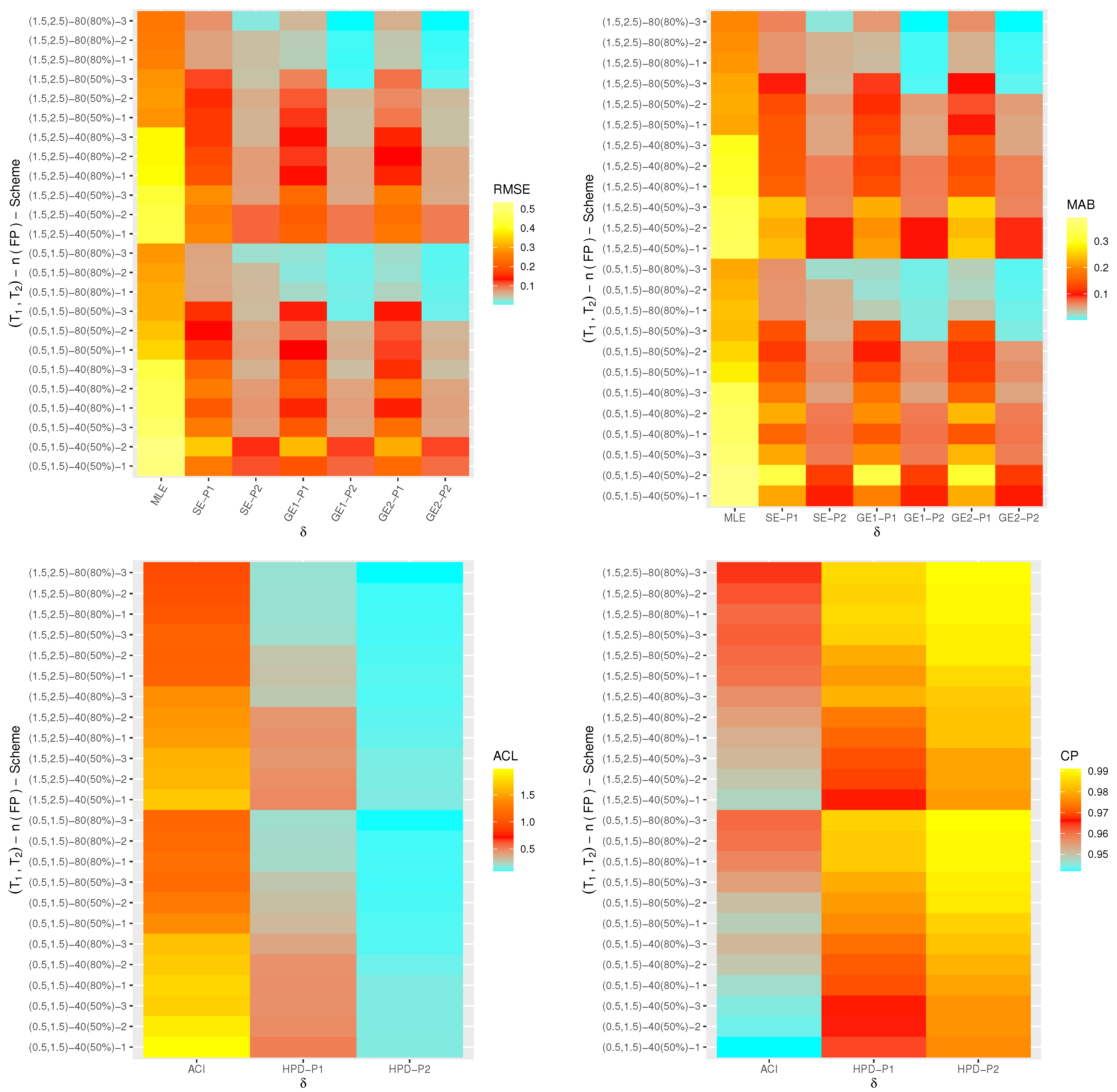
One of the best data visualization tools in $\mathsf{R}$ 4.2.2 software is known as a heat-map. Therefore, in this study, the simulated RMSEs, MABs, ACLs and CPs of $\delta$, $\mu$, $R\left(t\right)$ and $h\left(t\right)$ are plotted with heat-map and shown in Figure 4, Figure 5, Figure 6 and Figure 7, respectively. Also, the numerical results of $\delta$, $\mu$, $R\left(t\right)$ and $h\left(t\right)$ are also available in a Supplementary File. Some abbreviations of the proposed methods, for Prior-I (say P1) as an example, have been used such as: “SE-P1” refers to the Bayes estimates under SE loss; “GE1-P1” refers to the Bayes estimates under GE loss (for $\nu =-2$); “GE2-P1” refers to the Bayes estimates under GE loss (for $\nu =+2$) and “HPD-P1” refers to the HPD intervals.

From Figure 4, Figure 5, Figure 6 and Figure 7, in terms of the smallest RMSE, MAB and ACL values as well as the highest CP values, the following notes are drawn:

• A general observation in this study is that the acquired estimates of $\delta$, $\mu$, $R\left(t\right)$ or $h\left(t\right)$ have good behavior.
• Due to gamma informations, the Bayes point estimates (or their HPD credible interval estimates) of $\delta$, $\mu$, $R\left(t\right)$ or $h\left(t\right)$ behave satisfactory compared to the frequentist estimates.
• Comparing the variance values associated with priors I and II, it can be seen that the variance of Prior-II is lower than the other, thus the Bayes calculations from this prior provide good estimates.
• As n(or m) increases, both point and interval estimates of all unknown quantities perform sufficiently. A similar note is also obtained at ${\sum }_{i=1}^m{R}_i$ decreases.
• As $T_i,i=1,2$ increase, the RMSEs, MABs and ACLs of $\delta$, $\mu$, $R\left(t\right)$ and $h\left(t\right)$ decrease except for those associated with $R\left(t\right)$ in the case of MCMC estimates. Opposite behavior of $\delta$, $\mu$, $R\left(t\right)$ and $h\left(t\right)$ is also reached in the case of estimated CP values.
• Comparing the proposed censoring mechanisms, all calculated point/interval estimates of $\delta$, $\mu$, $R\left(t\right)$ or $h\left(t\right)$ are more efficient using Scheme 3 than others.
• As a summary, to estimate the IER parameters $\delta$, $\mu$, $R\left(t\right)$ or $h\left(t\right)$ in presence of data generated from Type-II generalized progressively hybrid censored sampling, the Bayes’ paradigm via M-H algorithm is recommended.

4. Real-Life Applications

To explain the usefulness of the suggested inferential methodologies and to illustrate the study findings’ relevance to actual phenomena, this section examines two real applications by evaluating real data sets collected from the engineering and chemistry areas. These applications stated that the suggested inferential methodologies, under the proposed censoring, perform adequately when utilized on real-life data.

4.1. Mechanical Components

This application analyzes an engineering data set representing the failure times of twenty mechanical components. This data was taken from Murthy et al. [32] and recently discussed by Alotaibi et al. [33] and Elshahhat et al. [34]. For convenience, each data point is multiplied by ten. The new transformed data are sorted an ascending order and presented in

Table 3. Failure data of 20 mechanical components.

0.67	0.68	0.76	0.81	0.84	0.85	0.85	0.86	0.89	0.98
0.98	1.14	1.14	1.15	1.21	1.25	1.31	1.49	1.60	4.85

. To examine whether fitting IER distribution to the data is appropriate or not, the Kolmogorov–Smirnov (K–S) test statistic and its p-value are computed.

First, from Table 3, the calculated MLEs of $\delta$ and $\mu$ with their standard errors (St.Errs) are 2.3896(0.7868) and 1.4970(0.3406), respectively, as well as the K–S (p-value) is 0.126(0.908). This result represents the fact that the IER model fits the mechanical components data adequately. Graphically, Figure 8 displays (i) the estimated and empirical reliability lines, and (ii) contour of the fitted log-likelihood function. As expected, Figure 8 supports our fitting findings and shows that the likelihood estimates $\widehat{\delta }\equiv 2.3896$ and $\widehat{\mu }\equiv 1.4970$ exist and unique.

Now, to explain the acquired estimates from the mechanical components data, based on $m=10$, $\mathbf{R}=\left(1^{*}10\right)$ and different choices of $T_i,i=1,2$, three artificial generalized-T2PH samples are generated and reported in

Table 4. Different generalized-T2PH samples from mechanical components data.

Sample	${\mathit{T}}_1\left({\mathit{d}}_1\right)$	${\mathit{T}}_2\left({\mathit{d}}_2\right)$	Censored Data	${\mathit{R}}^{*}$	${\mathit{T}}^{*}$
1	4.95(11)	5.00(11)	0.67, 0.76, 0.84, 0.85, 0.89, 0.98, 1.14, 1.21, 1.31, 1.60, 4.85	0	4.95
2	1.25(8)	1.65(10)	0.67, 0.76, 0.84, 0.85, 0.89, 0.98, 1.14, 1.21, 1.31, 1.60	0	1.60
3	1.00(6)	1.55(9)	0.67, 0.76, 0.84, 0.85, 0.89, 0.98, 1.14, 1.21, 1.31	2	1.55

. From Table 4, the offered point estimates (along their St.Errs) of $\delta$, $\mu$, $R\left(t\right)$ and $h\left(t\right)$ (at $t=1$) are reported in

Table 5. Point estimates of $\delta$, $\mu$, $R\left(t\right)$ and $h\left(t\right)$ from mechanical components data.

Sample	Par.	MLE		SE		GE
$\mathit{\nu }\to$						−3		−0.03		+3
		Est.	St.Err	Est.	St.Err	Est.	St.Err	Est.	St.Err	Est.	St.Err
1	$\delta$	1.4654	0.6467	1.3402	0.1931	1.3535	0.1119	1.3312	0.1342	1.3074	0.1580
	$\mu$	1.5668	0.4623	1.4556	0.1754	1.4661	0.1007	1.4476	0.1192	1.4284	0.1384
	$R\left(1\right)$	0.7096	0.0879	0.6991	0.0453	0.7015	0.0081	0.6975	0.0121	0.6931	0.0165
	$h\left(1\right)$	1.2112	0.3673	1.1887	0.1543	1.2074	0.0038	1.1796	0.0316	1.1512	0.0599
2	$\delta$	2.7224	1.6018	2.5983	0.1950	2.6066	0.1159	2.5939	0.1286	2.5808	0.1417
	$\mu$	2.0465	0.6121	1.9445	0.1695	1.9479	0.0987	1.9332	0.1134	1.9176	0.1289
	$R\left(1\right)$	0.6862	0.0917	0.6679	0.0453	0.6686	0.0176	0.6646	0.0216	0.6604	0.0258
	$h\left(1\right)$	1.6530	0.5449	1.6918	0.1777	1.7167	0.0636	1.6902	0.0372	1.6630	0.0100
3	$\delta$	2.1542	1.3272	2.0273	0.1947	2.0380	0.1163	2.0220	0.1322	2.0055	0.1487
	$\mu$	1.8663	0.6036	1.7621	0.1692	1.7721	0.0942	1.7572	0.1091	1.7417	0.1246
	$R\left(1\right)$	0.6963	0.0911	0.6810	0.0443	0.6835	0.0128	0.6797	0.0165	0.6757	0.0206
	$h\left(1\right)$	1.4715	0.5254	1.4846	0.1613	1.5020	0.0305	1.4762	0.0047	1.4501	0.0215

. Using noninformative priors, where $\mathcal{S}=$ 50,000 and ${\mathcal{S}}^{★}=$ 10,000, the MCMC estimates of $\delta$, $\mu$, $R\left(t\right)$ and $h\left(t\right)$ based on SE and GE (for $\nu (=-3,-0.03,+3)$) losses are also obtained, see Table 5. Also, in

Table 6. Interval estimates of $\delta$, $\mu$, $R\left(t\right)$ and $h\left(t\right)$ from mechanical components data.

Sample	Par.	ACI			HPD
		Lower	Upper	IL	Lower	Upper	IL
1	$\delta$	0.1980	2.7328	2.5349	1.0520	1.6329	0.5809
	$\mu$	0.6607	2.4730	1.8123	1.1967	1.7221	0.5254
	$R\left(1\right)$	0.5374	0.8819	0.3445	0.6131	0.7834	0.1702
	$h\left(1\right)$	0.4913	1.9310	1.4398	0.9049	1.4935	0.5886
2	$\delta$	0.4171	5.8619	5.4448	2.3134	2.8952	0.5818
	$\mu$	0.8469	3.2462	2.3992	1.6652	2.1975	0.5323
	$R\left(1\right)$	0.5065	0.8659	0.3594	0.5858	0.7472	0.1614
	$h\left(1\right)$	0.5851	2.7210	2.1358	1.3687	2.0411	0.6724
3	$\delta$	0.4471	4.7555	4.3084	1.7375	2.3032	0.5657
	$\mu$	0.6832	3.0494	2.3662	1.4869	2.0105	0.5236
	$R\left(1\right)$	0.5177	0.8748	0.3571	0.5986	0.7587	0.1602
	$h\left(1\right)$	0.4418	2.5012	2.0593	1.1731	1.7922	0.6191

, the 95% ACI as well as 95% HPD interval estimates (along their interval lengths (ILs)) are obtained. Table 5 and Table 6 stated that the acquired estimates of $\delta$, $\mu$, $R\left(t\right)$ and $h\left(t\right)$ developed by frequentist (or Bayes) approach are very close to each other.

Some properties for 40,000 remaining MCMC draws of $\delta$, $\mu$, $R\left(t\right)$ and $h\left(t\right)$ namely: mean, mode, first quartile $Q_1$, median, third quartile $Q_3$, standard-deviation (St.D) and skewness are computed, see

Table 7. Statistics for MCMC iterations of $\delta$, $\mu$, $R\left(t\right)$ and $h\left(t\right)$ from mechanical components data.

Sample	Par.	Mean	Mode	${\mathit{Q}}_1$	Median	${\mathit{Q}}_3$	St.D	Skewness
1	$\delta$	1.34023	0.95281	1.24522	1.34228	1.43862	0.14705	−0.12406
	$\mu$	1.45557	1.22232	1.36275	1.45175	1.54657	0.13566	0.10664
	$R\left(1\right)$	0.69911	0.71716	0.67074	0.70130	0.72989	0.04411	−0.30217
	$h\left(1\right)$	1.18868	0.97254	1.08139	1.18309	1.29140	0.15269	0.20700
2	$\delta$	2.59829	2.24704	2.49609	2.59927	2.70160	0.15033	0.00921
	$\mu$	1.94451	1.66521	1.85161	1.94356	2.03607	0.13535	0.05411
	$R\left(1\right)$	0.66789	0.62429	0.64126	0.66906	0.69711	0.04138	−0.25408
	$h\left(1\right)$	1.69184	1.74574	1.57329	1.68643	1.80312	0.17337	0.23730
3	$\delta$	2.02727	1.76272	1.92738	2.02779	2.12651	0.14760	0.04591
	$\mu$	1.76208	1.45968	1.67071	1.75966	1.85209	0.13325	0.07618
	$R\left(1\right)$	0.68098	0.62750	0.65406	0.68274	0.71047	0.04154	−0.27335
	$h\left(1\right)$	1.48463	1.55724	1.37154	1.47701	1.58965	0.16077	0.26114

. One of the most difficult difficulties in Bayesian MCMC computations is determining the level of convergence of the computed Markovian chain. Therefore, both the density as well as the trace plots of $\delta$, $\mu$, $R\left(t\right)$ and $h\left(t\right)$ are plotted, see Figure 9. Clearly; the sample mean is shown by a solid-line while the HPD interval bounds are depicted by dashed-lines.

Figure 9 shows that the simulated chains converge adequately and ${\mathcal{S}}^{★}$ sample has adequate size to eliminate the influence of the starting points. It also indicates that the distribution of estimates of $\delta$ and $\mu$ is fairly-symmetrical while that associated with $R\left(t\right)$ and $h\left(t\right)$ are negative- and positive-skewed, respectively.

4.2. Cumin Essential Oil

Cumin essential oil (CEO) is a super spicy oil that needs to be handled with care. It is extracted through steam distillation and is clear in color. Cuminaldehyde is the bioactive component in CEO and is obtained using an experimental distillation plant. Following Panahi [35], we shall present the analysis of the CEO data set to clarify the study goal. In

Table 8. Cuminaldehyde data from the CEO.

3.386	3.796	3.789	3.960	4.354	4.481	5.091	3.655	4.246	4.523	4.758	5.589
6.676	6.845	6.498	5.398	6.668	6.757	5.939	5.787	7.089	5.054	4.867	4.985

, the cuminaldehyde data measured on a Pye Unicam/Philips PU 4500 gas chromatograph is reported. To verify whether the IER distribution fits the cuminaldehyde data, the K–S statistic (with its p-value) and MLEs (with their St.Errs) of $\delta$ and $\mu$ based on the cuminaldehyde data are computed. However, using Table 8, the MLEs (St.Errs) of $\delta$ and $\mu$ are 8.5785(3.7247) and 64.883(12.260), respectively. Furthermore, the K–S (p-value) is 0.125(0.805). It implies that the IER lifetime model fits the cuminaldehyde data significantly. Additionally, Figure 10 confirmed that our fitted results and demonstrated that the estimates $\widehat{\delta }$ and $\widehat{\mu }$ are exist and unique. For benefit, we propose using these estimates $\widehat{\delta }\equiv 8.5785$ and $\widehat{\mu }\equiv 64.883$ to carried out any upcoming calculations.

Now different generalized-T2PH samples (when $m=12$, $\mathbf{R}=\left(1^{*}12\right)$ and several points of $T_i,i=1,2$) are generated from cuminaldehyde data and listed in

Table 9. Different generalized-T2PH samples from cuminaldehyde data.

Sample	${\mathit{T}}_1\left({\mathit{d}}_1\right)$	${\mathit{T}}_2\left({\mathit{d}}_2\right)$	Censored Data	${\mathit{R}}^{*}$	${\mathit{T}}^{*}$
1	7.2(13)	7.5(13)	3.386, 3.789, 3.960, 4.354, 4.523, 4.867, 5.054, 5.398, 5.787, 6.498, 6.676, 6.845, 7.089	7.2	0
2	6.5(11)	7.2(12)	3.386, 3.789, 3.960, 4.354, 4.523, 4.867, 5.054, 5.398, 5.787, 6.498, 6.676, 6.845	6.845	0
3	6.2(9)	6.8(11)	3.386, 3.789, 3.960, 4.354, 4.523, 4.867, 5.054, 5.398, 5.787, 6.498, 6.676	6.8	2

. From Table 9, the derived estimators of $\delta$, $\mu$, $R\left(t\right)$ and $h\left(t\right)$ (at $t=5$) are evaluated obtained via likelihood and Bayesian approaches are presented in

Table 10. Point estimates of $\delta$, $\mu$, $R\left(t\right)$ and $h\left(t\right)$ from cuminaldehyde data.

Sample	Par.	MLE		SE		GE
$\mathit{\nu }\to$						−3		−0.03		+3
		Est.	St.Err	Est.	St.Err	Est.	St.Err	Est.	St.Err	Est.	St.Err
1	$\delta$	5.0778	2.5010	4.9248	0.2297	4.9307	0.1471	4.9219	0.1559	4.9128	0.1650
	$\mu$	66.290	12.124	66.138	0.2321	66.139	0.1507	66.138	0.1514	66.137	0.1521
	$R\left(4\right)$	0.9220	0.0339	0.9235	0.0031	0.9235	0.0016	0.9235	0.0016	0.9235	0.0015
	$h\left(4\right)$	0.1697	0.0563	0.1658	0.0071	0.1660	0.0037	0.1657	0.0040	0.1653	0.0043
2	$\delta$	4.0875	2.0227	3.9287	0.2343	3.9363	0.1512	3.9251	0.1625	3.9135	0.1740
	$\mu$	61.594	12.920	61.436	0.2359	61.436	0.1584	61.435	0.1592	61.435	0.1599
	$R\left(4\right)$	0.9158	0.0406	0.9182	0.0042	0.9182	0.0024	0.9182	0.0023	0.9181	0.0023
	$h\left(4\right)$	0.1711	0.0612	0.1657	0.0091	0.1661	0.0051	0.1656	0.0056	0.1651	0.0061
3	$\delta$	3.1790	1.4369	3.0201	0.2339	3.0298	0.1492	3.0153	0.1637	3.0003	0.1787
	$\mu$	56.471	10.278	56.312	0.2361	56.312	0.1585	56.311	0.1593	56.311	0.1601
	$R\left(4\right)$	0.9097	0.0375	0.9132	0.0059	0.9132	0.0035	0.9132	0.0035	0.9132	0.0034
	$h\left(4\right)$	0.1695	0.0565	0.1622	0.0118	0.1627	0.0067	0.1619	0.0075	0.1611	0.0083

and

Table 11. Interval estimates of $\delta$, $\mu$, $R\left(t\right)$ and $h\left(t\right)$ from cuminaldehyde data.

Sample	Par.	ACI			HPD
		Lower	Upper	IL	Lower	Upper	IL
1	$\delta$	0.1759	9.9797	9.8037	4.5950	5.2730	0.6780
	$\mu$	42.527	90.052	47.525	65.797	66.484	0.6864
	$R\left(4\right)$	0.8555	0.9885	0.1330	0.9183	0.9289	0.0106
	$h\left(4\right)$	0.0593	0.2800	0.2206	0.1543	0.1778	0.0235
2	$\delta$	0.1231	8.0519	7.9287	3.5875	4.2610	0.6735
	$\mu$	36.272	86.917	50.645	61.096	61.774	0.6780
	$R\left(4\right)$	0.8363	0.9953	0.1590	0.9112	0.9251	0.0139
	$h\left(4\right)$	0.0513	0.2910	0.2397	0.1512	0.1802	0.0290
3	$\delta$	0.3628	5.9952	5.6324	2.6943	3.3658	0.6716
	$\mu$	36.326	76.615	40.289	55.972	56.649	0.6776
	$R\left(4\right)$	0.8362	0.9833	0.1470	0.9039	0.9227	0.0188
	$h\left(4\right)$	0.0588	0.2802	0.2214	0.1438	0.1802	0.0364

. Improper gamma priors to illustrate the Bayes estimates are considered here also. It is noted, from Table 10 and Table 11, that the offered estimates of $\delta$, $\mu$, $R\left(t\right)$ or $h\left(t\right)$ exhibit the same pattern since they seem to be close to each other. Interval estimates of the same unknown parameters have a similar pattern of behavior. As a result, there is no significant difference between the suggested estimates, which is also an expected finding owing to the absence of further historical data that may be used.

Using the same vital statistics described in Section 4.1, based on 40,000 MCMC variates, several properties of $\delta$, $\mu$, $R\left(t\right)$ and $h\left(t\right)$ are calculated, see

Table 12. Statistics for MCMC iterations of $\delta$, $\mu$, $R\left(t\right)$ and $h\left(t\right)$ from cuminaldehyde data.

Sample	Par.	Mean	Mode	${\mathit{Q}}_1$	Median	${\mathit{Q}}_3$	St.D	Skewness
1	$\delta$	4.92477	4.78637	4.81165	4.92498	5.03747	0.17136	0.00749
	$\mu$	66.1384	65.8608	66.0193	66.1387	66.2583	0.17612	−0.00900
	$R\left(4\right)$	0.92353	0.92433	0.92172	0.92350	0.92532	0.00269	0.00983
	$h\left(4\right)$	0.16577	0.16328	0.16192	0.16579	0.16973	0.00596	−0.00406
2	$\delta$	3.92874	3.65246	3.81278	3.93027	4.04089	0.17234	−0.01738
	$\mu$	61.4356	61.1458	61.3167	61.4362	61.5532	0.17435	0.00399
	$R\left(4\right)$	0.91816	0.92233	0.91581	0.91818	0.92052	0.00353	0.03267
	$h\left(4\right)$	0.16573	0.15621	0.16081	0.16576	0.17056	0.00737	−0.02234
3	$\delta$	3.02009	2.74396	2.90488	3.02150	3.13214	0.17159	−0.02325
	$\mu$	56.3117	56.0220	56.1925	56.3125	56.4294	0.17444	0.00396
	$R\left(4\right)$	0.91322	0.91941	0.91005	0.91320	0.91641	0.00478	0.04269
	$h\left(4\right)$	0.16220	0.14937	0.15605	0.16227	0.16826	0.00928	−0.02747

. In Figure 11, for each sample in Table 9, the density as well as trace plots of MCMC iterations of $\delta$, $\mu$, $R\left(t\right)$ and $h\left(t\right)$ are shown. It demonstrates that the Markovian iterations converge superiorly and shows that the acquired estimates of $\delta$, $\mu$, $R\left(t\right)$ or $h\left(t\right)$ are distributed fairly symmetrically.

5. Conclusions

This article discusses the examination of a generalized progressive Type-II hybrid censored test where the lifespans of the testing products have an inverted exponentiated Rayleigh model. Besides the issue of estimating model parameters, the present study has also taken into account the estimating issues of reliability and failure functions of the proposed model. The likelihood approach has been used to get acquire both point and asymptotic estimates of the objective parameters. From a Bayes’ point of view, both symmetric and asymmetric Bayes estimates, based on asymmetric and symmetric loss functions, of the unknown parameters have been developed using a hybrid Monte-Carlo Markov-Chain algorithm. Also, two-sided highest posterior interval estimators of the same parameters have also been cerated. Through valuable simulation experiments, the efficiency of various estimating strategies has been established. Numerical evaluations show that the acquired Bayes points and credible estimates behave satisfactorily. Two $\mathsf{R}$ packages, namely ‘$\mathsf{maxLik}$’ and ‘$\mathsf{coda}$’, have been installed to evaluate the suggested theoretical results. Two applications, based on real data sets from various fields, namely engineering and chemistry, have been examined to demonstrate the utility of the suggested model in real-world applications. As a summary, in the presence of a sample produced through the proposed censoring, the Bayes framework is advised for estimating the model parameters of life of the inverted exponentiated Rayleigh model. In the future, it would be interesting to examine the inferential concerns of the same model utilized for other statistical challenges, such as accelerating life tests, competing risks, etc.

References

1. Bain, L.J.; Engelhardt, M. Statistical Analysis of Reliability and Life-Testing Models, 2nd ed.; Marcel Dekker: New York, NY, USA, 1991. [Google Scholar]
2. Epstein, B. Truncated life tests in the exponential case. Ann. Math. Stat. 1954, 25, 555–564. [Google Scholar] [CrossRef]
3. Childs, A.; Chandrasekar, B.; Balakrishnan, N.; Kundu, D. Exact likelihood inference based on Type-I and Type-II hybrid censored samples from the exponential distribution. Ann. Inst. Stat. Math. 2003, 55, 319–330. [Google Scholar] [CrossRef]
4. Balakrishnan, N.; Cramer, E. The Art of Progressive Censoring; Springer: Birkhäuser, NY, USA, 2014. [Google Scholar]
5. Ng, H.K.T.; Kundu, D.; Chan, P.S. Statistical analysis of exponential lifetimes under an adaptive Type-II progressive censoring scheme. Nav. Res. Logist. 2009, 56, 687–698. [Google Scholar] [CrossRef] [Green Version]
6. Lee, K.; Sun, H.; Cho, Y. Exact likelihood inference of the exponential parameter under generalized Type II progressive hybrid censoring. J. Korean Stat. Soc. 2016, 45, 123–136. [Google Scholar] [CrossRef]
7. Ashour, S.; Elshahhat, A. Bayesian and non-Bayesian estimation for Weibull parameters based on generalized Type-II progressive hybrid censoring scheme. Pak. J. Stat. Oper. Res. 2016, 12, 213–226. [Google Scholar]
8. Ateya, S.; Mohammed, H. Prediction under Burr-XII distribution based on generalized Type-II progressive hybrid censoring scheme. J. Egypt. Math. Soc. 2018, 26, 491–508. [Google Scholar]
9. Seo, J.I. Objective Bayesian analysis for the Weibull distribution with partial information under the generalized Type-II progressive hybrid censoring scheme. Commun. Stat.-Simul. Comput. 2020, 51, 5157–5173. [Google Scholar] [CrossRef]
10. Cho, S.; Lee, K. Exact Likelihood Inference for a Competing Risks Model with Generalized Type II Progressive Hybrid Censored Exponential Data. Symmetry 2021, 13, 887. [Google Scholar] [CrossRef]
11. Nagy, M.; Bakr, M.E.; Alrasheedi, A.F. Analysis with applications of the generalized Type-II progressive hybrid censoring sample from Burr Type-XII model. Math. Probl. Eng. 2022, 2022, 1241303. [Google Scholar] [CrossRef]
12. Wang, L.; Zhou, Y.; Lio, Y.; Tripathi, Y.M. Inference for Kumaraswamy Distribution under Generalized Progressive Hybrid Censoring. Symmetry 2022, 14, 403. [Google Scholar] [CrossRef]
13. Elshahhat, A.; Mohammed, H.S.; Abo-Kasem, O.E. Reliability Inferences of the Inverted NH Parameters via Generalized Type-II Progressive Hybrid Censoring with Applications. Symmetry 2022, 14, 2379. [Google Scholar] [CrossRef]
14. Alotaibi, R.; Rezk, H.; Elshahhat, A. Computational Analysis for Fréchet Parameters of Life from Generalized Type-II Progressive Hybrid Censored Data with Applications in Physics and Engineering. Symmetry 2023, 15, 348. [Google Scholar] [CrossRef]
15. Ghitany, M.E.; Tuan, V.K.; Balakrishnan, N. Likelihood estimation for a general class of inverse exponentiated distributions based on complete and progressively censored data. J. Stat. Comput. Simul. 2014, 84, 96–106. [Google Scholar] [CrossRef]
16. Rastogi, M.K.; Tripathi, Y.M. Estimation for an inverted exponentiated Rayleigh distribution under type II progressive censoring. J. Appl. Stat. 2014, 41, 2375–2405. [Google Scholar] [CrossRef]
17. Kayal, T.; Tripathi, Y.M.; Rastogi, M.K. Estimation and prediction for an inverted exponentiated Rayleigh distribution under hybrid censoring. Commun. Stat.-Theory Methods 2018, 47, 1615–1640. [Google Scholar] [CrossRef]
18. Maurya, R.K.; Tripathi, Y.M.; Sen, T.; Rastogi, M.K. On progressively censored inverted exponentiated Rayleigh distribution. J. Stat. Comput. Simul. 2019, 89, 492–518. [Google Scholar] [CrossRef]
19. Gao, S.; Gui, W. Parameter estimation of the inverted exponentiated Rayleigh distribution based on progressively first-failure censored samples. Int. J. Syst. Assur. Eng. Manag. 2019, 10, 925–936. [Google Scholar] [CrossRef]
20. Maurya, R.K.; Tripathi, Y.M.; Rastogi, M.K. Estimation and prediction for a progressively first-failure censored inverted exponentiated Rayleigh distribution. J. Stat. Theory Pract. 2019, 13, 39. [Google Scholar] [CrossRef]
21. Gao, S.; Yu, J.; Gui, W. Pivotal inference for the inverted exponentiated Rayleigh distribution based on progressive type-II censored data. Am. J. Math. Manag. Sci. 2020, 39, 315–328. [Google Scholar] [CrossRef]
22. Panahi, H.; Moradi, N. Estimation of the inverted exponentiated Rayleigh distribution based on adaptive Type II progressive hybrid censored sample. J. Comput. Appl. Math. 2020, 364, 112345. [Google Scholar] [CrossRef]
23. Fan, J.; Gui, W. Statistical inference of inverted exponentiated Rayleigh distribution under joint progressively type-II censoring. Entropy 2022, 24, 171. [Google Scholar] [CrossRef] [PubMed]
24. Kundu, D.; Joarder, A. Analysis of Type-II progressively hybrid censored data. Comput. Stat. Data Anal. 2006, 50, 2509–2528. [Google Scholar] [CrossRef]
25. Childs, A.; Chandrasekar, B.; Balakrishnan, N. Exact likelihood inference for an exponential parameter under progressive hybrid censoring schemes. In Statistical Models and Methods for Biomedical and Technical Systems; Vonta, F., Nikulin, M., Limnios, N., Huber-Carol, C., Eds.; Birkhäuser: Boston, MA, US, 2008; pp. 319–330. [Google Scholar]
26. Plummer, M.; Best, N.; Cowles, K.; Vines, K. CODA: Convergence diagnosis and output analysis for MCMC. R News 2006, 6, 7–11. [Google Scholar]
27. Henningsen, A.; Toomet, O. maxLik: A package for maximum likelihood estimation in R. Comput. Stat. 2011, 26, 443–458. [Google Scholar] [CrossRef]
28. Lawless, J.F. Statistical Models and Methods For Lifetime Data, 2nd ed.; John Wiley and Sons: Hoboken, NJ, USA, 2003. [Google Scholar]
29. Calabria, R.; Pulcini, G. An engineering approach to Bayes estimation for the Weibull distribution. Microelectron. Reliab. 1994, 34, 789–802. [Google Scholar] [CrossRef]
30. Van Ravenzwaaij, D.; Cassey, P.; Brown, S.D. A simple introduction to Markov Chain Monte–Carlo sampling. Psychon. Bull. Rev. 2018, 25, 143–154. [Google Scholar] [CrossRef] [Green Version]
31. Chen, M.H.; Shao, Q.M. Monte Carlo estimation of Bayesian credible and HPD intervals. J. Comput. Graph. Stat. 1999, 8, 69–92. [Google Scholar]
32. Murthy, D.N.P.; Xie, M.; Jiang, R. Weibull Models; Wiley Series in Probability and Statistics; Wiley: Hoboken, NJ, USA, 2004. [Google Scholar]
33. Alotaibi, R.; Nassar, M.; Rezk, H.; Elshahhat, A. Inferences and Engineering Applications of Alpha Power Weibull Distribution Using Progressive Type-II Censoring. Mathematics 2022, 10, 2901. [Google Scholar] [CrossRef]
34. Elshahhat, A.; El-Sherpieny, E.S.A.; Hassan, A.S. The Pareto-Poisson Distribution: Characteristics, Estimations and Engineering Applications. Sankhya A 2023, 85, 1058–1099. [Google Scholar] [CrossRef]
35. Panahi, H. Inference for exponentiated Pareto distribution based on progressive first-failure censored data with application to cumin essential oil data. J. Stat. Manag. Syst. 2018, 21, 1433–1457. [Google Scholar] [CrossRef]
Figure 1. The log-likelihood functions of δ and μ from generalized-T2PH censored data.
Axioms 12 00565 g001
Figure 2. Autocorrelation plots of δ , μ , R ( t ) and h ( t ) (after burn-in) from generalized-T2PH censored data.
Axioms 12 00565 g002
Figure 3. Evaluating plots for 12,000 MCMC draws of δ and μ from generalized-T2PH censored data.
Axioms 12 00565 g003aAxioms 12 00565 g003b
Figure 4. Heat-maps for the estimation outputs of δ .
Axioms 12 00565 g004
Figure 5. Heat-maps for the estimation outputs of μ .
Axioms 12 00565 g005
Figure 6. Heat-maps for the estimation outputs of R ( t ) .
Axioms 12 00565 g006
Figure 7. Heat-maps for the estimation outputs of h ( t ) .
Axioms 12 00565 g007
Figure 8. Empirical/Fitted reliability parameter (left-side); Contour (right-side) plots from mechanical components data.
Axioms 12 00565 g008
Figure 9. Density (left) and Trace (right) plots of δ , μ , R ( t ) and h ( t ) from mechanical components data.
Axioms 12 00565 g009
Figure 10. Empirical/Fitted reliability parameter (left-side); Contour (right-side) plots from cuminaldehyde data.
Axioms 12 00565 g010
Figure 11. Density (left) and Trace (right) plots of δ , μ , R ( t ) and h ( t ) from cuminaldehyde data.
Axioms 12 00565 g011