Article

Inverse Unit Teissier Distribution: Theory and Practical Examples

1
Department of Quantitative Analysis, College of Business Administration, King Saud University, P.O. Box 71115, Riyadh 11587, Saudi Arabia
2
Mathematics and Computer Science Department, Faculty of Science, Beni-Suef University, Beni-Suef 62521, Egypt
3
Department of Statistics, Faculty of Sciences, Selcuk University, Konya 42130, Turkey
4
Department of Mathematics, Faculty of Science, Tanta University, Tanta 31527, Egypt
5
Department of Mathematics, Université de Caen Normandie, Campus II, Science 3, 14032 Caen, France
6
Basic and Applied Science Institute, Arab Academy for Science, Technology and Maritime Transport (AASTMT), Alexandria P.O. Box 1029, Egypt
*
Author to whom correspondence should be addressed.
Axioms 2023, 12(5), 502; https://doi.org/10.3390/axioms12050502
Submission received: 20 March 2023 / Revised: 12 May 2023 / Accepted: 19 May 2023 / Published: 20 May 2023

Abstract

:
In this paper, we emphasize a new one-parameter distribution with support as [ 1 , + ) . It is constructed from the inverse method applied to an understudied one-parameter unit distribution, the unit Teissier distribution. Some properties are investigated, such as the mode, quantiles, stochastic dominance, heavy-tailed nature, moments, etc. Among the strengths of the distribution are the following: (i) the closed-form expressions and flexibility of the main functions, and in particular, the probability density function is unimodal and the hazard rate function is increasing or unimodal; (ii) the manageability of the moments; and, more importantly, (iii) it provides a real alternative to the famous Pareto distribution, also with support as [ 1 , + ) . Indeed, the proposed distribution has different functionalities but also benefits from the heavy-right-tailed nature, which is demanded in many applied fields (finance, the actuarial field, quality control, medicine, etc.). Furthermore, it can be used quite efficiently in a statistical setting. To support this claim, the maximum likelihood, Anderson–Darling, right-tailed Anderson–Darling, left-tailed Anderson–Darling, Cramér–Von Mises, least squares, weighted least-squares, maximum product of spacing, minimum spacing absolute distance, and minimum spacing absolute-log distance estimation methods are examined to estimate the unknown unique parameter. A Monte Carlo simulation is used to compare the performance of the obtained estimates. Additionally, the Bayesian estimation method using an informative gamma prior distribution under the squared error loss function is discussed. Data on the COVID mortality rate and the timing of pain relief after receiving an analgesic are considered to illustrate the applicability of the proposed distribution. Favorable results are highlighted, supporting the importance of the findings.

1. Introduction

In order to create adaptable models for data analysis, a significant area of statistics seeks to create distributions with novel traits. In fact, a new distribution can present a fresh modeling viewpoint and a clearer picture of the underlying mechanisms generating the data. As a result, a number of new distributions have been introduced recently, including those in [1,2,3].
Among the famous lifetime distributions, the Teissier (T) distribution (also called the Muth (M) distribution) was established in [4] to simulate the frequency of death related to aging. Laurent [5] investigated its classification based on life expectancy and demonstrated its applicability to demographic datasets. Muth [6] employed this distribution to analyze dependability. Reference [7] determined the main features of the T distribution. They referred to it as the M distribution, although they might have overlooked publications [4,5]. As a matter of fact, scientists have paid little consideration to the T distribution. However, it is of interest because it may be preferable to the one-parameter exponential distribution when modeling data with a subordinate increasing hazard rate function (HRF). Among the existing developments based on the T distribution, let us mention the power M distribution studied in [8], transmuted M-generated class of distributions proposed in [9], new M-generated class of distributions elaborated in [10], exponentiated power M distribution discussed in [11], inverse power M distribution investigated in [12] and the truncated M generated family of distributions emphasized in [13]. More recently, Krishna et al. [14] used the T distribution for creating an intriguing unit distribution, i.e., a distribution with support as [ 0 , 1 ] , the unit T distribution (UTD). This work has motivated the present paper as explained later. Basically, the UTD is the distribution of the random variable Y = e Z , where Z is a random variable that follows the T distribution. The cumulative distribution function (CDF) of the UTD is indicated as follows:
G ( y ) = y θ e 1 y θ , y [ 0 , 1 ] ,
which is completed with G ( y ) = 0 for y < 0 and G ( y ) = 1 for y > 1 , with a shape parameter θ such that θ > 0 , and the corresponding probability density function (PDF) is given by
g ( y ) = θ e 1 y θ y 2 θ 1 1 y θ , y [ 0 , 1 ] ,
with g ( y ) = 0 for y [ 0 , 1 ] 
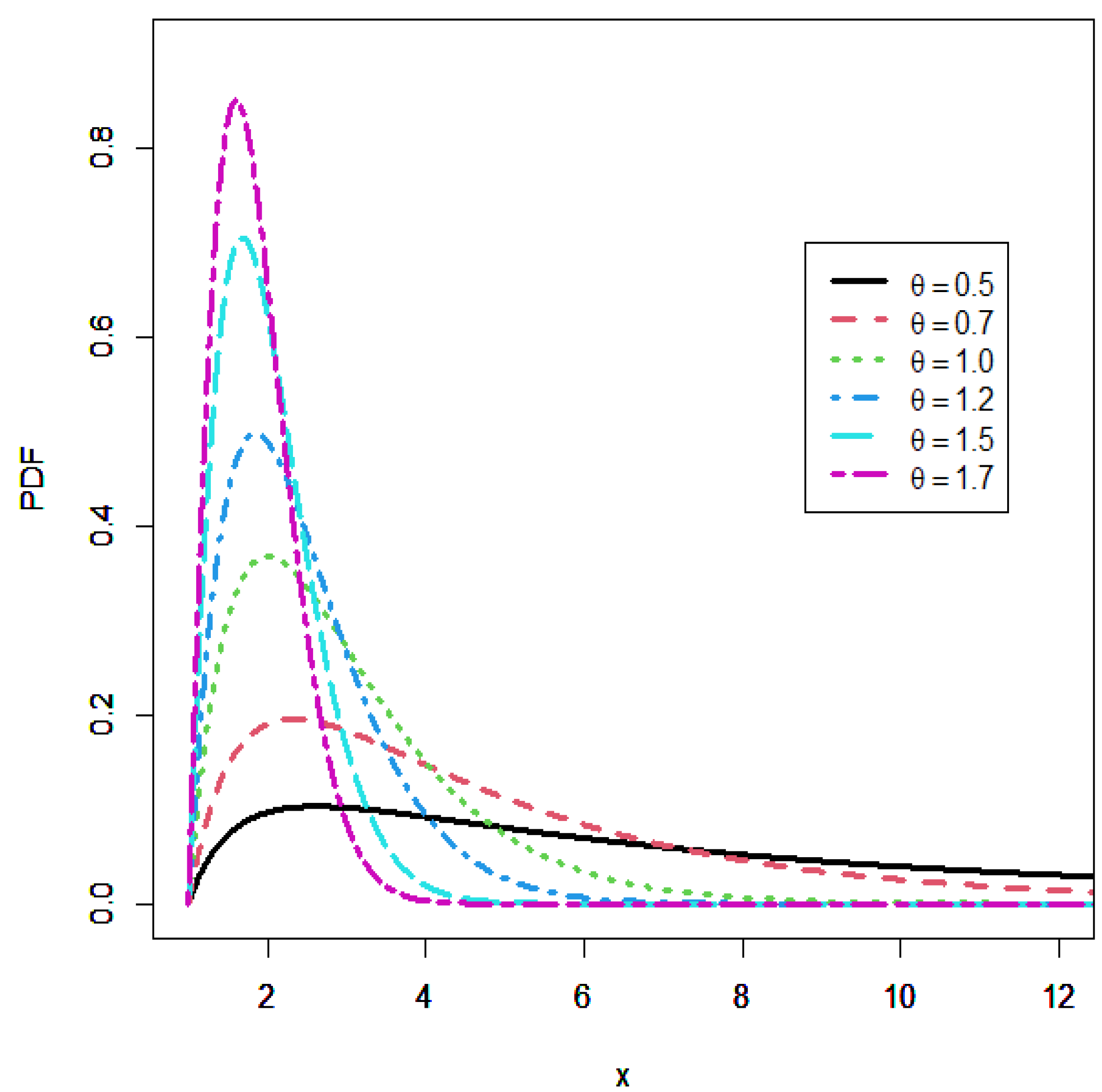
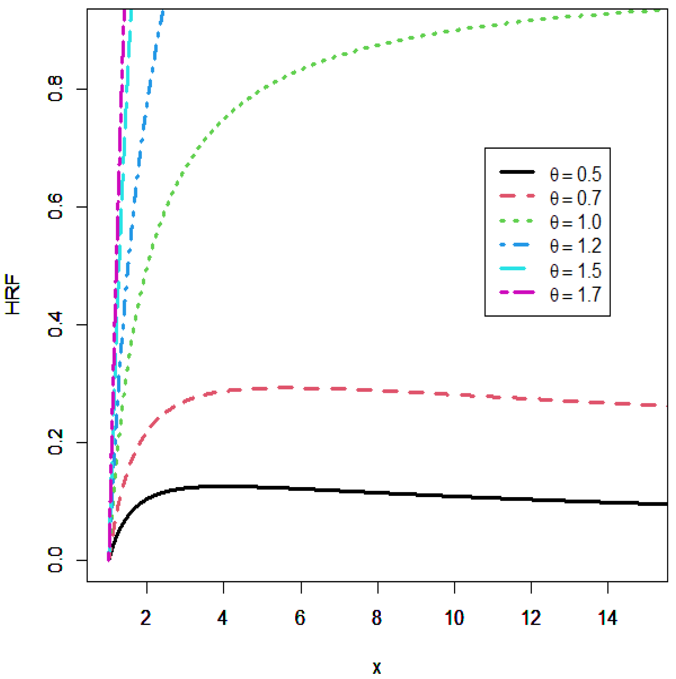
. The UTD stands out from the other unit distributions because of the following combined advantages: (i) It depends on only one parameter. (ii) It possesses closed-form expressions for the PDF, CDF, HRF, moments, inequality-type functions, and entropy measures. (iii) It has flexible PDF and HRF, with a HRF presenting non-monotone shapes, including the bathtub shape and N-shapes.
On a more general level, several methods exist to transform a known distribution into a new distribution. Among the most significant of them is the inverse transformation method based on the standard inverse (or ratio) function. More precisely, a new distribution is obtained by performing the transformation X = 1 / Y , where Y represents a random variable that follows an existing distribution. Many flexible new distributions are derived by this method, such as the inverse Student (IT) distribution, inverse exponential (IE) distribution, inverse Cauchy (IC) distribution, inverse Fisher (IF) distribution, inverse chi-squared (ICS) distribution (see [15]), inverse Lindley (IL) distribution (see [16]), inverse Xgamma (IXG) distribution (see [17]), inverse power Lindley (IPL) distribution (see [18]), inverted Kumaraswamy (IK) distribution (see [19]), inverted exponentiated Weibull (IEW) distribution (see [20]), inverse Weibull generator (IW-G) of distributions (see [21]), inverted Nadarajah-Haghighi (INH) distribution (see [22]), inverse power Lomax (IP) distribution (see [23]), inverted Topp–Leone (ITL) distribution (see [24]), inverse Maxwell (IM) distribution (see [25]), inverse Nakagami-m (IN-m) distribution (see [26]), inverse Pareto (IP) distribution (see [27]), etc. In full generality, the inverse distributions are especially beneficial when working with variables having a limited range of values, such as time or distance measurements. They are often used in practice to model the lifetime of a particular product or the distribution of insurance claims.
On the other hand, we recall that the Pareto (P) distribution is a distribution that describes the occurrence of extreme events, also known as the power law distribution. It was introduced by the Italian economist Vilfredo Pareto to explain the distribution of wealth in society. The P distribution is characterized by a shape parameter, which determines the rate at which the distribution decays and has the support [ 1 , + ) in its basic definition. The larger the value of this parameter, the faster the distribution decays. This means that the P distribution has a heavy tail, with a few very large values and many small values. The P distribution has applications in various fields, such as finance, physics, and biology, among others. In particular, it is used quite successfully to model the frequency of occurrence of events that follow a power law (a priori), such as earthquakes, city populations, or income distributions. Modern references on this topic are [28,29,30].
In this paper, using the above information as the motor, a new inverse distribution based on the UTD is introduced, and we name it the inverse UTD (IUTD). As a basic presentation, it constitutes a new one-parameter distribution with support as [ 1 , + ) . It provides a solid alternative to the P distribution as described above. We will emphasize that the IUTD has the same possibility of applications as the P distribution but with more perspective in terms of functionalities and modeling. In the first part, we explore the main functions and properties of the IUTD. In particular, we show that the corresponding PDF can be unimodal and the HRF can be unimodal or increasing. This functional flexibility is an advantage in a modeling sense. We determine its quantile function (QF) from which we derive the quantiles, stochastic dominance, heavy-tailed nature, moments (incomplete and complete), etc. The second part is statistically oriented. Ten estimation methods are developed and employed to estimate the unique parameter involved. We prove their efficiency through a classical simulation approach. Finally, using two real-world data sets as examples, the application demonstrates the superiority of the IUTD over other well-known distributions, including the T and P distributions.
The current paper is organized as follows: In Section 2, we formulate the mathematical foundations of the IUTD, mainly by presenting and studying the PDF, CDF, and HRF. Its mathematical properties are investigated in Section 3. In Section 4, the estimation methods are examined to find the estimates of the unique parameter, and a Monte Carlo simulation is conducted to observe their behavior. In 
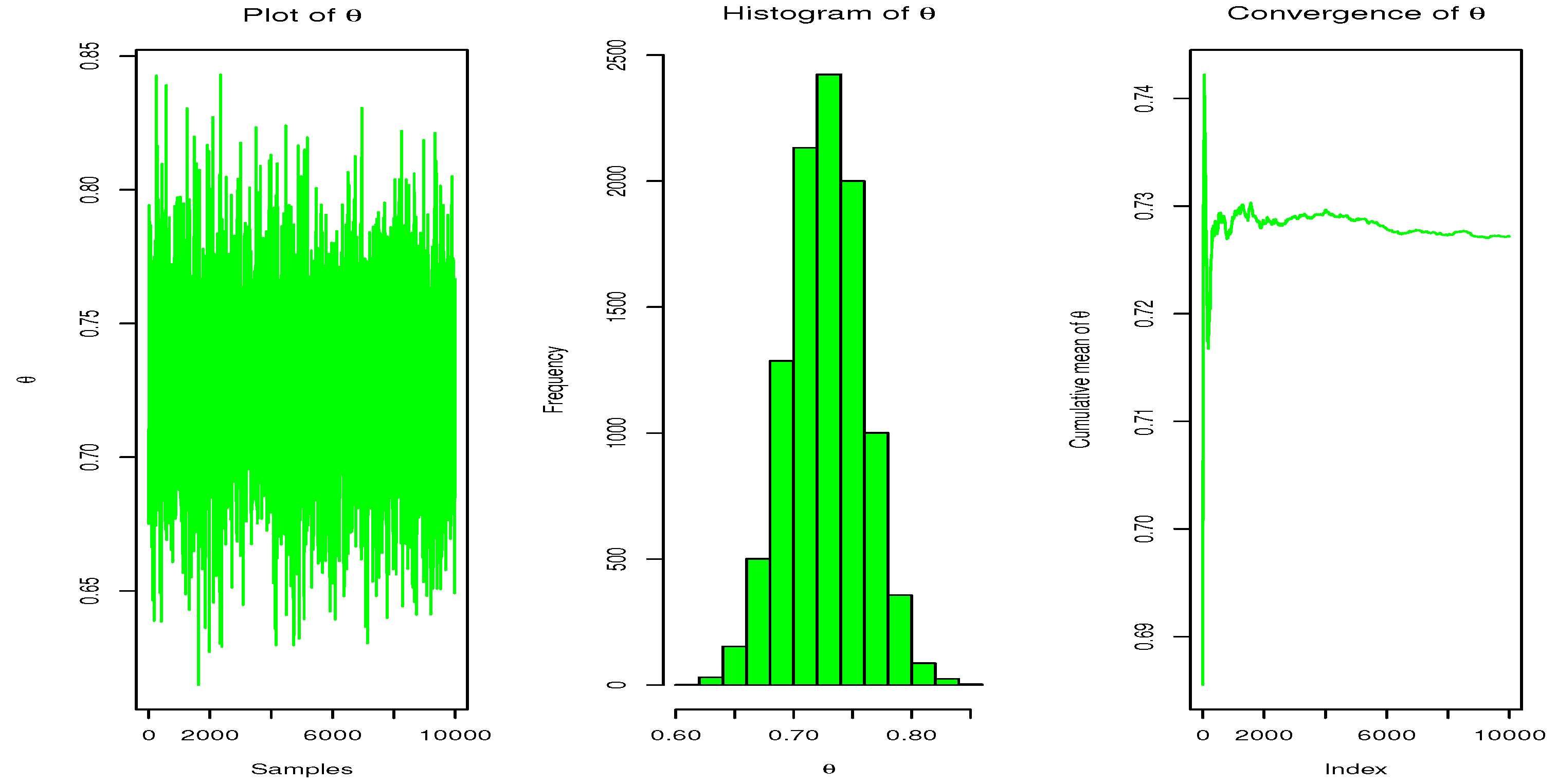
Section 5, the Bayesian estimation method using the informative gamma prior distribution with the squared error loss function is discussed. In Section 6, two practical examples are carried out. The conclusion of this study is included in Section 7.

2. Distribution Formulation

2.1. Cumulative Distribution and Probability Density Functions

As sketched in the introductory section, the IUTD is defined by the CDF of X = 1 / Y , where Y is a random variable that follows the UTD. We can also present the IUTD as the distribution of the random variable X = e Z , where Z is a random variable that follows the T distribution. Thus, the support of the IUTD is [ 1 , + ) . Based on the CDF in (1), for any x 1 , the CDF of the IUTD is obtained by the following equation: F ( x ) = P ( X x ) = 1 P ( Y 1 / x ) , i.e.,
F ( x ) = 1 e 1 x θ x θ .
We naturally put F ( x ) = 0 for x < 1 , and we recall that θ is a shape parameter satisfying θ > 0 . At this development step, we point out the simplicity of the definition of F ( x ) and its originality; to our knowledge, it has not been considered in the existing literature. Some additional features will be described in the whole paper.
The corresponding PDF is defined by f ( x ) = d F ( x ) / ( d x ) , i.e.,
f ( x ) = θ e 1 x θ x θ 1 x θ 1 , x 1 .
We naturally put f ( x ) = 0 for x < 1 . This PDF contains important information about the modeling capabilities of the IUTD. The most significant of them concerns the possible forms and shapes of this PDF. The main results on this aspect are in the proposition below.
Proposition 1. 
The PDF of the IUTD as defined in (4) is exclusively unimodal.
Proof. 
To begin, let us remark that lim x 1 f ( x ) = lim x + f ( x ) = 0 (because of the exponential term for x + ). Since f ( x ) 0 for any x [ 1 , + ) , this implies that f ( x ) is at least unimodal (it can be multimodal at this step). By differentiation of f ( x ) with respect to x, we obtain
d d x f ( x ) = θ e 1 x θ x θ 2 θ x θ 3 x θ + x θ + θ 1 .
By solving the equation d f ( x ) / ( d x ) = 0 , we find only one solution, which is given by
x = 2 1 / θ 5 θ 2 2 θ + 1 + 3 θ 1 θ 1 / θ .
Since 5 θ 2 2 θ + 1 ( θ 1 ) 2 = 4 θ 2 > 0 , we have ( 5 θ 2 2 θ + 1 + 3 θ 1 ) / ( 2 θ ) > 1 , and the solution above belongs to [ 1 , + ) . Moreover, since lim x 1 f ( x ) = lim x + f ( x ) = 0 , it is a maximum point for f ( x ) . Hence, the PDF of the IUTD is exclusively unimodal. □
Proposition 1 reveals an important difference with the P distribution: the PDF of the P distribution is exclusively decreasing, whereas the one of the IUTD is exclusively unimodal. For this reason, for data values in [ 1 , + ) , the IUTD is more adequate than the P distribution if the empirical unimodality seems present.
Based on the proof of Proposition 1, we define the mode of the IUTD as follows:
M * = 2 1 / θ 5 θ 2 2 θ + 1 + 3 θ 1 θ 1 / θ .
In order to visually support the result in Proposition 1, Figure 1 gives some plots for f ( x ) by considering several values for θ .
From this figure, it is clear that f ( x ) is unimodal, as established in Proposition 1.

2.2. Survival and Hazard Rate Functions

The survival function (SF) of the IUTD is defined as S ( x ) = 1 F ( x ) , i.e.,
S ( x ) = e 1 x θ x θ , x 1 ,
and S ( x ) = 1 for x < 1 . Its HRF follows as h ( x ) = f ( x ) / S ( x ) , i.e.,
h ( x ) = θ x θ 1 x , x 1 ,
and h ( x ) = 0 for x < 1 . Again, we notice the simplicity of this function, which is only defined with the power version of x and θ . Like the PDF, its analytical behavior is decisive for understanding the modeling capacities of the IUTD.
Proposition 2. 
The HRF of the IUTD as defined in (6) can be increasing or unimodal.
Proof. 
To begin, let us perform an asymptotic study. We have lim x 1 h ( x ) = 0 and
lim x + h ( x ) = + if θ > 1 1 if θ = 1 0 if θ ( 0 , 1 ) .
As a direct consequence, it is at least unimodal for θ ( 0 , 1 ) (and can be increasing for θ 1 ). To go further, let us consider the first derivative of h ( x ) with respect to x, i.e.,
d d x h ( x ) = θ x 2 1 + ( θ 1 ) x θ .
Based on it:
  • For any θ 1 , we clearly have d h ( x ) / ( d x ) > 0 , implying that h ( x ) is increasing.
  • For any θ ( 0 , 1 ) , the equation d h ( x ) / ( d x ) = 0 has the following solution: x = ( 1 θ ) 1 / θ , which belongs to [ 1 , + ) . Since lim x 1 h ( x ) = lim x + h ( x ) = 0 and h ( x ) 0 , it is a maximum point. In other words, in this case, h ( x ) is unimodal, ending the proof.
Here again, Proposition 2 shows a major difference with the P distribution: the HRF of the P distribution is exclusively decreasing, i.e., equal to θ / x , whereas the one of the IUTD is increasing or unimodal. In this aspect, the IUTD can be viewed as the counterpart of the P distribution.
Figure 2 supports graphically the result in Proposition 2 by showing plots of h ( x ) with several values for θ .
From this figure, we can well distinguish the two cases: increasing and unimodal, depending on θ 1 and θ ( 0 , 1 ) , respectively.

3. Mathematical Properties

In this section, we drive some important properties of the IUTD, such as the QF along with its use to have randomly generated datasets, the heavy-tailed nature, stochastic dominance, and moments (incomplete and complete), along with two important inequality curves and asymmetry and flatness measures.

3.1. Quantile Function

The QF of the IUTD is defined as the inverse function of the CDF in (3). It is indicated in the next result.
Proposition 3. 
The QF of the IUTD is expressed as
Q ( p ) = W p 1 e 1 / θ , p [ 0 , 1 ] ,
where W ( x ) is the Lambert function, i.e., defined as W ( x ) e W ( x ) = x .
Proof. 
As the definition of an inverse function, Q ( p ) must satisfy the following functional equation: F [ Q ( p ) ] = p for any p [ 0 , 1 ] . Based on it, the following equivalence holds:
F [ Q ( p ) ] = p 1 e 1 [ Q ( p ) ] θ [ Q ( p ) ] θ = p e [ Q ( p ) ] θ [ Q ( p ) ] θ = p 1 e [ Q ( p ) ] θ = W p 1 e Q ( p ) = W p 1 e 1 / θ .
The desired expression is obtained. □
By considering this QF, we can determine many quantile characteristics of the IUTD (median, i.e., Q ( 0.5 ) , quartiles, i.e., Q ( 0.25 ) , Q ( 0.75 ) , whiskers, etc.). Furthermore, we can easily generate random values from a random variable X that follows the IUTD distribution using the inversion method. Indeed, by considering n values from a random variable P that follows the uniform distribution over [ 0 , 1 ] , say p 1 , , p n , then n values from X are x 1 , , x n , where
x i = Q ( p i ) = W p i 1 e 1 / θ , i = 1 , 2 , , n .

3.2. Heavy-Tailed Nature

The following result is about the heavy-tailed nature of the IUTD.
Proposition 4. 
The IUTD is a heavy-tailed distribution for θ ( 0 , 1 ] , and it is not for θ > 1 .
Proof. 
To begin, for any t > 0 , we have
I = 1 + e t x f ( x ) d x = 1 + θ e 1 x ( x θ 1 t ) x θ 1 x θ 1 d x .
  • For θ ( 0 , 1 ) , any t > 0 , and x + , we have x θ 1 t t , implying that the term e t x is dominant in the integrated function; by the Riemann integral rules, we have I = + , meaning that the UTD is heavy-tailed.
  • For θ = 1 and any t > 1 , the same argument holds: the UTD is heavy-tailed.
  • For θ > 1 , any t > 0 , and x + , we have x θ 1 t + , implying that the term e x θ is dominant in the integrated function; by the Riemann integral rules, we have I < + , meaning that the UTD is not heavy-tailed.
This result is important because it makes a strong difference with the P distribution, which is the most famous distribution with support as [ 1 , + ) . Indeed, the P distribution is exclusively a heavy-tailed distribution for all the values of the involved parameter, whereas the IUTD is more flexible on this aspect, and the modulation of θ can make the difference in a data fitting scenario. This point will be illustrated concretely with real-life datasets in Section 6.

3.3. Stochastic Dominance

The IUTD has comprehensible stochastic dominances (first-order and HRF), which are listed in the proposition below.
Proposition 5. 
  • Let us set F ( x ; θ ) = F ( x ) . Then, for any x R and θ 2 θ 1 > 0 , we have
    F ( x ; θ 1 ) F ( x ; θ 2 ) .
  • Let us set h ( x ; θ ) = h ( x ) . Then, for any x R and θ 2 θ 1 > 0 , we have
    h ( x ; θ 1 ) h ( x ; θ 2 ) .
Proof. 
  • For any x < 1 , it is clear that F ( x ; θ 1 ) = F ( x ; θ 2 ) = 0 . Let us investigate the monotonicity of F ( x ; θ ) with respect to θ for any x 1 . We have
    d d θ F ( x ; θ ) = e 1 x θ x θ ( x θ 1 ) log ( x ) 0 .
    Therefore, F ( x ; θ ) is increasing with respect to θ , and as a result, for any θ 2 θ 1 > 0 , we have F ( x ; θ 1 ) F ( x ; θ 2 ) .
  • Similarly, for any x < 1 , it is clear that h ( x ; θ 1 ) = h ( x ; θ 2 ) = 0 . Let us investigate the monotonicity of h ( x ; θ ) with respect to θ for any x 1 . We have
    d d θ h ( x ; θ ) = x θ 1 + a x a log ( x ) x 0 .
    Therefore, h ( x ; θ ) is increasing with respect to θ , and as a result, for any θ 2 θ 1 > 0 , we have h ( x ; θ 1 ) h ( x ; θ 2 ) .
This ends the proof. □
The demonstrated stochastic dominances are useful to compare the related models with respect to the parameter θ . All the information on this topic can be found in [31].

3.4. Incomplete and Complete Moments

Incomplete moments are a useful tool in probability and statistics for calculating the moments of a distribution up to a certain order. Unlike complete moments, which are calculated from the entire distribution, incomplete moments are calculated from a truncated distribution that is limited to a specific range or interval. The incomplete moments related to the IUTD are given in the following proposition.
Proposition 6. 
Let X be a random variable that follows the IUTD distribution, k be a positive integer and t 1 . Then the k-th incomplete moment of X at t is defined by ρ k ( t ) = E ( X k 1 { X t } ) , where E represents the mathematical expectation operator and can be expressed as
ρ k ( t ) = 1 t k + θ e 1 t θ + k e θ γ k θ + 1 , t θ γ k θ + 1 , 1 ,
where γ ( a , z ) = 0 z t a 1 e t d t for any a > 0 and z > 0 .
Proof. 
By applying an integration by parts without expressing the involved functions, we obtain
ρ k ( t ) = 1 t x k f ( x ) d x = x k S ( x ) x = 1 x = t + k 1 t x k 1 S ( x ) d x = 1 t k S ( t ) + k 1 t x k 1 S ( x ) d x .
We have S ( t ) = e 1 t θ t θ . Moreover, by applying the change of variables u = x θ , we have
1 t x k 1 S ( x ) d x = 1 t x k 1 e 1 x θ x θ d x = e θ 1 t θ u k / θ e u d u = e θ γ k θ + 1 , t θ γ k θ + 1 , 1 .
By combining the above identities, we obtain the desired result. □
One of the advantages of the IUTD is that it has a closed-form expression of its incomplete moments. Some consequences of this property are described below.
From the incomplete moments, we immediately derive the complete moments. Indeed, the k-th complete moment of a random variable X that follows the IUTD is given by μ k = E ( X k ) , and we have
μ k = lim t + ρ k ( t ) = lim t + 1 t k + θ e 1 t θ + k e θ γ k θ + 1 , t θ γ k θ + 1 , 1 = 1 + k e θ Γ k θ + 1 , 1 ,
where Γ ( a , z ) = z + t a 1 e t d t for any a > 0 and z > 0 .
The incomplete moments can be used to determine various residual life functions, and important quantities in survival analysis. In particular, the first incomplete and complete moments are important for expressing the Lorenz and Bonferroni curves, which are, respectively, defined as follows: L C 1 ( t ) = ρ 1 ( t ) / μ 1 and B C 2 ( t ) = ρ 1 ( t ) / ( p μ 1 ) . It is also used to establish the mean residual life ( M R L ( t ) = [ 1 ρ 1 ( t ) ] / S ( t ) t ), and the mean waiting time ( M W T ( t ) = t ρ 1 ( t ) / F ( t ) ).
Additionally, based on the complete moments, we can calculate the j-th central moment of X by utilizing moments around the origin as follows:
μ j = E [ ( X μ 1 ) j ] = l = 0 j ( 1 ) l j l μ 1 l μ j l .
Then, the skewness and kurtosis coefficients are given by SK = μ 3 / μ 2 3 / 2 and KU = μ 4 / μ 2 2 . They are crucial to identifying the asymmetry and flatness of the IUTD distribution, respectively.
To end this portion, in Table 1, we provide a numerical study of the most important quantities presented in the sections above.
From this table, we can note that there is a certain numerical flexibility in the mode, skewness, and kurtosis. In particular, since SK can be negative or positive, we conclude that the IUTD can be left or right skewed, and since KU can be less or greater than 3, all the kurtosis states are reached, i.e., leptokurtic, mesokurtic, and platykurtic.

3.5. Order Statistics

In this subsection, some results on the order statistics of the IUTD are examined. Let X 1 , X 2 , , X n be a random sample from the IUTD and X ( 1 ) X ( 2 ) X ( n ) represent the related order statistics. Let r = 1 , 2 , , n . Then the CDF and PDF of the r-th order statistic, that is X ( r ) , are obtained as
F X ( r ) ( x ) = i = r n j = 0 n i ( 1 ) j n i n i j 1 e 1 x θ x θ i + j
and
f X ( r ) ( x ) = θ e 1 x θ x θ 1 x θ 1 B ( r , n r + 1 ) i = 0 n r ( 1 ) i n r i 1 e 1 x θ x θ r + i 1 ,
where B a , b is the standard beta function, i.e., B ( a , b ) = 0 1 t a 1 ( 1 t ) b 1 d t with a > 0 and b > 0 . For r = 1 and r = n , the CDF and PDF of X ( 1 ) = min X 1 , X 2 , , X n and X ( n ) = max X 1 , X 2 , , X n are achieved, respectively.

4. Estimation of the Parameter

This section presents the traditional estimation methods for the unique parameter of the IUTD and their application in a simulation setting.

4.1. Methods

Ten estimation methods are considered. For each of the methods, the obtained estimate is derived by optimizing an objective function for a maximum or minimum value. The consider estimation setting and the definitions of the functions to be optimized are presented below.
Let x 1 , , x n be a random sample of values from a random variable X that follows the IUTD. Then, an estimate of θ is calculated using the maximum-likelihood estimation (MLE) by maximizing the following function:
log L = i = 1 n log [ f ( x i ) ] = i = 1 n 1 x i θ + ( θ 1 ) i = 1 n log x i + i = 1 n log x i θ 1 + n log ( θ ) .
This function corresponds to the logarithmic likelihood function of the IUTD.
Let x ( 1 ) , , x ( n ) be an ordered sample of values from a random variable that follows the IUTD. Then, an estimate of θ is calculated using the Anderson–Darling estimation (ADE) by minimizing the following function:
A = n 1 n i = 1 n ( 2 i 1 ) log [ F ( x ( i ) ) ] + log [ S ( x ( i ) ) ] = n 1 n i = 1 n ( 2 i 1 ) log 1 e 1 x ( i ) θ x ( i ) θ + 1 x ( i ) θ + θ log x ( i ) .
See [32] for more details on the ADE.
An estimate of θ is calculated using the right-tailed Anderson–Darling estimation (RADE) by minimizing the following function:
R = n 2 2 i = 1 n F ( x ( i ) ) 1 n i = 1 n ( 2 i 1 ) log [ S ( x ( i ) ) ] = n 2 2 i = 1 n 1 e 1 x ( i ) θ x ( i ) θ 1 n i = 1 n ( 2 i 1 ) 1 x ( i ) θ + θ log x ( i ) .
We also refer to [32] for the technical details on this method.
An estimate of θ is calculated using the left-tailed Anderson–Darling estimation (LTADE) by minimizing the following function:
L = 3 2 n + 2 i = 1 n F ( x ( i ) ) 1 n i = 1 n ( 2 i 1 ) log [ F ( x ( i ) ) ] = 3 2 n + 2 i = 1 n 1 e 1 x ( i ) θ x ( i ) θ 1 n i = 1 n ( 2 i 1 ) log 1 e 1 x ( i ) θ x ( i ) θ .
See [33].
An estimate of θ is calculated using the Cramér–Von Mises estimation (CVME) by minimizing the following function:
C = 1 12 n + i = 1 n F ( x ( i ) ) 2 i 1 2 n 2 = 1 12 n + i = 1 n 1 e 1 x ( i ) θ x ( i ) θ 2 i 1 2 n 2 .
More elements on this method can be found in [34].
An estimate of θ is calculated using the least-squares estimation (LSE) by minimizing the following function:
V = i = 1 n F ( x ( i ) ) i n + 1 2 = i = 1 n 1 e 1 x ( i ) θ x ( i ) θ i n + 1 2 .
More information on this method is given in [35].
An estimate of θ is calculated using the weighted least-squares estimation (WLSE) by minimizing the following function:
W = i = 1 n ( n + 1 ) 2 ( n + 2 ) i ( n i + 1 ) F ( x ( i ) ) i n + 1 2 = i = 1 n ( n + 1 ) 2 ( n + 2 ) i ( n i + 1 ) 1 e 1 x ( i ) θ x ( i ) θ i n + 1 2 .
See again [35].
An estimate of θ is calculated using the maximum product of spacing estimation (MPSE) by maximizing the following function:
δ = 1 n + 1 i = 1 n + 1 log ( Φ i ) ,
where
Φ i = F ( x ( i ) ) F ( x ( i 1 ) ) = e 1 x ( i 1 ) θ x ( i 1 ) θ e 1 x ( i ) θ x ( i ) θ .
The details on this estimation method are available in [36].
An estimate of θ is calculated using the minimum spacing absolute distance estimation (MSADE) by minimizing the following function:
Υ 1 = i = 1 n + 1 Φ i 1 n + 1 .
See [37].
An estimate of θ is calculated using the minimum spacing absolute-log distance estimation method (MSALDE) by minimizing the following function:
Υ 2 = i = 1 n + 1 log ( Φ i ) log 1 n + 1 .
See [37].
All these methods have proved themselves in various parametric estimation scenarios. In the next part, we illustrate this claim in the context of the IUTD.

4.2. Numerical Simulation

In our simulation study, we employ the following sample sizes: n = 20 , 40, 80, 120, 160, 200, 250, and 350, and we randomly generate datasets by using the inversion method (see Section 3.1) and the following parameter values: θ = 0.25 , 0.75 , 1.0 , 2.5 , and 4.0 . We wish to look at the behavior of the considered estimation methods. We use the following measures to assess their effectiveness:
  • Average of bias:
    B i a s = 1 H i = 1 H | θ ^ i θ | ,
    where H represents the number of iterations and θ ^ i is the considered estimate for θ at the i-th iteration sample.
  • Mean squared error:
    M S E = 1 H i = 1 H ( θ ^ i θ ) 2 .
  • Mean relative error:
    M R E = 1 H i = 1 H | θ ^ i θ | θ .
  • Average absolute difference:
    D a b s = 1 n H i = 1 H j = 1 n | F ( x i j ; θ ) F ( x i j ; θ ^ ) | ,
    where F ( x ; θ ) = F ( x ) , x i j denotes the values obtained at the i-th iteration sample and j-th component of this sample and θ ^ is the average estimate.
  • Maximum absolute difference:
    D m a x = 1 H i = 1 H max j = 1 , , n | F ( x i j ; θ ) F ( x i j ; θ ^ ) | .
  • Average squared absolute error:
    A S A E = 1 H i = 1 H | x ( i ) x ^ ( i ) | x ( n ) x ( 1 ) ,
    where x ( i ) is the i-th ordered values (in increasing order) and x ^ ( i ) = Q ( i / ( n + 1 ) ; θ ^ i ) , where Q ( x ; θ ) = Q ( x ) is the QF of the IUTD.
In addition, for all the parameter combinations, we determine the percentile bootstrap confidence interval length (CIL) for both small and large sample sizes. The R programming software is used to do all of these calculations (see [38]).
Table 2, Table 3, Table 4, Table 5 and Table 6 show the results of our simulation using the ten estimation techniques (in them and hereafter, the notation e x stands for × 10 x ). From these tables, we have following comments hold:
  • It should be noted that all the parameter estimation methods are quite reliable and very close to their actual values; they are precise.
  • All the calculated measures for every scenario under consideration decrease as n rises.
  • The performance of each estimation method is excellent in finding the parameter.
  • Table 7 displays the overall ranks for all estimation strategies, and we see that the MLE is the best for the values of the parameters assessed in our study (total score of 65.0).
These results justify the use of the ML estimation method for the statistical practice of the IUTD.
Table 2. Numerical values of the simulation for the IUTD with θ = 0.25 .
nEst.MLEADECVMEMPSEOLSERTADEWLSELTADEMSADEMSALDE
20BIAS 0 . 01801 { 2 } 0 . 01924 { 5 } 0 . 02233 { 9 } 0 . 01751 { 1 } 0 . 0221 { 8 } 0 . 01921 { 4 } 0 . 02125 { 6 } 0 . 02474 { 10 } 0 . 021835 { 7 } 0 . 018933 { 3 }
MSE 0 . 00054 { 2 } 6 e 04 { 4.5 } 0 . 00085 { 8 } 0 . 00049 { 1 } 0 . 00079 { 7 } 6 e 04 { 4.5 } 0 . 00074 { 6 } 0 . 00101 { 10 } 0 . 000869 { 9 } 0 . 000566 { 3 }
MRE 0 . 07202 { 2 } 0 . 07695 { 5 } 0 . 08931 { 9 } 0 . 07005 { 1 } 0 . 08842 { 8 } 0 . 07684 { 4 } 0 . 08499 { 6 } 0 . 09896 { 10 } 0 . 087339 { 7 } 0 . 075733 { 3 }
CIL 0 . 08885 { 2 } 0 . 0941 { 5 } 0 . 10581 { 7 } 0 . 0821 { 1 } 0 . 10606 { 8 } 0 . 08899 { 3 } 0 . 10071 { 6 } 0 . 16145 { 10 } 0 . 11374 { 9 } 0 . 09233 { 4 }
D a b s 0 . 04326 { 2 } 0 . 04742 { 5 } 0 . 0533 { 9 } 0 . 0432 { 1 } 0 . 05299 { 8 } 0 . 04613 { 3 } 0 . 05037 { 6 } 0 . 05692 { 10 } 0 . 0516 { 7 } 0 . 04736 { 4 }
D m a x 0 . 06332 { 1 } 0 . 06925 { 4 } 0 . 0789 { 9 } 0 . 0637 { 2 } 0 . 07855 { 8 } 0 . 06834 { 3 } 0 . 07481 { 6 } 0 . 08607 { 10 } 0 . 07764 { 7 } 0 . 06937 { 5 }
ASAE 0 . 04918 { 3 } 0 . 06303 { 7 } 0 . 06803 { 8 } 0 . 04772 { 2 } 0 . 06938 { 9 } 0 . 05354 { 5 } 0 . 06091 { 6 } 0 . 07825 { 10 } 0 . 05227 { 4 } 0 . 04759 { 1 }
R a n k s 14 { 2 } 40 . 5 { 6 } 57 { 9 } 9 { 1 } 54 { 8 } 31 . 5 { 4 } 40 { 5 } 68 { 10 } 48 { 7 } 23 { 3 }
40BIAS 0 . 01305 { 2 } 0 . 01377 { 6 } 0 . 01403 { 7 } 0 . 01226 { 1 } 0 . 01488 { 8 } 0 . 01314 { 3 } 0 . 01364 { 4 } 0 . 01716 { 10 } 0 . 016157 { 9 } 0 . 013705 { 5 }
MSE 0 . 00026 { 2 } 3 e 04 { 5.5 } 0 . 00033 { 7 } 0 . 00024 { 1 } 0 . 00037 { 8 } 0 . 00027 { 3 } 3 e 04 { 5.5 } 0 . 00048 { 10 } 0 . 00043 { 9 } 0 . 000297 { 4 }
MRE 0 . 05218 { 2 } 0 . 05508 { 6 } 0 . 05613 { 7 } 0 . 04903 { 1 } 0 . 05951 { 8 } 0 . 05257 { 3 } 0 . 05457 { 4 } 0 . 06864 { 10 } 0 . 064626 { 9 } 0 . 054822 { 5 }
CIL 0 . 05996 { 2 } 0 . 06619 { 5 } 0 . 07239 { 8 } 0 . 05766 { 1 } 0 . 07208 { 7 } 0 . 0622 { 3 } 0 . 06784 { 6 } 0 . 08669 { 10 } 0 . 07696 { 9 } 0 . 06583 { 4 }
D a b s 0 . 03146 { 2 } 0 . 03337 { 5 } 0 . 03394 { 7 } 0 . 03017 { 1 } 0 . 03642 { 8 } 0 . 03185 { 3 } 0 . 03318 { 4 } 0 . 04111 { 10 } 0 . 03921 { 9 } 0 . 03375 { 6 }
D m a x 0 . 04689 { 2 } 0 . 04969 { 5 } 0 . 05045 { 7 } 0 . 0447 { 1 } 0 . 05386 { 8 } 0 . 04752 { 3 } 0 . 04932 { 4 } 0 . 06139 { 10 } 0 . 05848 { 9 } 0 . 05027 { 6 }
ASAE 0 . 02731 { 2 } 0 . 03399 { 7 } 0 . 03657 { 8 } 0 . 02722 { 1 } 0 . 04011 { 9 } 0 . 03068 { 3 } 0 . 03297 { 6 } 0 . 04125 { 10 } 0 . 03155 { 5 } 0 . 03134 { 4 }
R a n k s 14 { 2 } 43 . 5 { 6 } 49 { 7 } 7 { 1 } 54 { 8 } 21 { 3 } 37 . 5 { 5 } 68 { 10 } 57 { 9 } 34 { 4 }
80BIAS 0 . 00844 { 1.5 } 0 . 00892 { 3 } 0 . 01007 { 5 } 0 . 00925 { 4 } 0 . 0111 { 9 } 0 . 00844 { 1.5 } 0 . 01008 { 6 } 0 . 01218 { 10 } 0 . 010728 { 8 } 0 . 010322 { 7 }
MSE 0 . 00012 { 1.5 } 0 . 00013 { 3.5 } 0 . 00017 { 7 } 0 . 00013 { 3.5 } 2 e 04 { 9 } 0 . 00012 { 1.5 } 0 . 00016 { 5 } 0 . 00024 { 10 } 0 . 000187 { 8 } 0 . 000168 { 6 }
MRE 0 . 03377 { 2 } 0 . 03568 { 3 } 0 . 04027 { 5 } 0 . 03701 { 4 } 0 . 0444 { 9 } 0 . 03376 { 1 } 0 . 04031 { 6 } 0 . 04874 { 10 } 0 . 042913 { 8 } 0 . 041289 { 7 }
CIL 0 . 04187 { 2 } 0 . 04649 { 4 } 0 . 05062 { 8 } 0 . 0404 { 1 } 0 . 05052 { 7 } 0 . 04376 { 3 } 0 . 04683 { 5 } 0 . 05675 { 10 } 0 . 05412 { 9 } 0 . 04697 { 6 }
D a b s 0 . 02047 { 2 } 0 . 02177 { 3 } 0 . 02423 { 5 } 0 . 02278 { 4 } 0 . 02665 { 9 } 0 . 02038 { 1 } 0 . 02453 { 6 } 0 . 02942 { 10 } 0 . 02594 { 8 } 0 . 02536 { 7 }
D m a x 0 . 03046 { 1 } 0 . 03239 { 3 } 0 . 03629 { 5 } 0 . 03392 { 4 } 0 . 03998 { 9 } 0 . 03056 { 2 } 0 . 03652 { 6 } 0 . 04391 { 10 } 0 . 03893 { 8 } 0 . 03772 { 7 }
ASAE 0 . 01595 { 2 } 0 . 02098 { 7 } 0 . 02129 { 9 } 0 . 01589 { 1 } 0 . 02108 { 8 } 0 . 01745 { 4 } 0 . 01872 { 6 } 0 . 02531 { 10 } 0 . 01798 { 5 } 0 . 01737 { 3 }
R a n k s 12 { 1 } 26 . 5 { 4 } 44 { 7 } 21 . 5 { 3 } 61 { 9 } 14 { 2 } 40 { 5 } 69 { 10 } 54 { 8 } 43 { 6 }
120BIAS 0 . 00718 { 4 } 0 . 00715 { 3 } 0 . 00867 { 8 } 0 . 00702 { 1 } 0 . 00834 { 7 } 0 . 00703 { 2 } 0 . 0076 { 5 } 0 . 00911 { 10 } 0 . 009037 { 9 } 0 . 008234 { 6 }
MSE 8 e 05 { 2.5 } 8 e 05 { 2.5 } 0 . 00012 { 8 } 8 e 05 { 2.5 } 0 . 00011 { 7 } 8 e 05 { 2.5 } 9 e 05 { 5 } 0 . 00013 { 9 } 0 . 000138 { 10 } 0 . 000103 { 6 }
MRE 0 . 02874 { 4 } 0 . 02861 { 3 } 0 . 03469 { 8 } 0 . 02808 { 1 } 0 . 03335 { 7 } 0 . 02813 { 2 } 0 . 0304 { 5 } 0 . 03646 { 10 } 0 . 036149 { 9 } 0 . 032934 { 6 }
CIL 0 . 03381 { 2 } 0 . 03767 { 4 } 0 . 04106 { 7 } 0 . 03335 { 1 } 0 . 04106 { 8 } 0 . 03531 { 3 } 0 . 03808 { 5 } 0 . 04615 { 10 } 0 . 04361 { 9 } 0 . 03858 { 6 }
D a b s 0 . 01738 { 3 } 0 . 01748 { 4 } 0 . 02094 { 8 } 0 . 01718 { 1 } 0 . 02029 { 7 } 0 . 0172 { 2 } 0 . 01851 { 5 } 0 . 02223 { 10 } 0 . 02191 { 9 } 0 . 02021 { 6 }
D m a x 0 . 02594 { 3 } 0 . 02598 { 4 } 0 . 03134 { 8 } 0 . 02565 { 2 } 0 . 03026 { 7 } 0 . 02554 { 1 } 0 . 02759 { 5 } 0 . 0331 { 10 } 0 . 03273 { 9 } 0 . 0301 { 6 }
ASAE 0 . 01145 { 1 } 0 . 01427 { 7 } 0 . 0148 { 8 } 0 . 01167 { 2 } 0 . 01482 { 9 } 0 . 01354 { 5 } 0 . 0137 { 6 } 0 . 01627 { 10 } 0 . 01346 { 4 } 0 . 01198 { 3 }
R a n k s 24 . 5 { 3 } 32 . 5 { 4 } 50 { 8 } 15 . 5 { 1 } 47 { 7 } 22 . 5 { 2 } 41 { 6 } 64 { 10 } 54 { 9 } 34 { 5 }
160BIAS 0 . 00631 { 3 } 0 . 00661 { 4 } 0 . 00703 { 7 } 0 . 00593 { 1 } 0 . 0072 { 8 } 0 . 00624 { 2 } 0 . 00686 { 5 } 0 . 00842 { 10 } 0 . 007673 { 9 } 0 . 006958 { 6 }
MSE 6 e 05 { 2 } 7 e 05 { 4.5 } 8 e 05 { 7.5 } 6 e 05 { 2 } 8 e 05 { 7.5 } 6 e 05 { 2 } 7 e 05 { 4.5 } 0 . 00011 { 10 } 9.7 e 05 { 9 } 7.5 e 05 { 6 }
MRE 0 . 02523 { 3 } 0 . 02643 { 4 } 0 . 0281 { 7 } 0 . 02372 { 1 } 0 . 02879 { 8 } 0 . 02496 { 2 } 0 . 02743 { 5 } 0 . 03366 { 10 } 0 . 030693 { 9 } 0 . 02783 { 6 }
CIL 0 . 02926 { 2 } 0 . 03273 { 4 } 0 . 03541 { 8 } 0 . 0289 { 1 } 0 . 03531 { 7 } 0 . 03076 { 3 } 0 . 03311 { 5 } 0 . 03995 { 10 } 0 . 03748 { 9 } 0 . 03365 { 6 }
D a b s 0 . 01533 { 3 } 0 . 01603 { 4 } 0 . 01706 { 6 } 0 . 01451 { 1 } 0 . 01756 { 8 } 0 . 01517 { 2 } 0 . 01664 { 5 } 0 . 02045 { 10 } 0 . 01871 { 9 } 0 . 01709 { 7 }
D m a x 0 . 02287 { 3 } 0 . 02395 { 4 } 0 . 02546 { 7 } 0 . 02161 { 1 } 0 . 02612 { 8 } 0 . 02267 { 2 } 0 . 02488 { 5 } 0 . 03049 { 10 } 0 . 02786 { 9 } 0 . 02542 { 6 }
ASAE 0 . 00903 { 1 } 0 . 01064 { 6 } 0 . 01171 { 9 } 0 . 00911 { 2 } 0 . 01132 { 8 } 0 . 00994 { 4 } 0 . 01088 { 7 } 0 . 01276 { 10 } 0 . 00998 { 5 } 0 . 00946 { 3 }
R a n k s 18 { 2.5 } 32 . 5 { 4 } 52 . 5 { 7 } 10 { 1 } 55 . 5 { 8 } 18 { 2.5 } 38 . 5 { 5 } 61 { 10 } 60 { 9 } 39 { 6 }
200BIAS 0 . 00537 { 1 } 0 . 00624 { 4 } 0 . 0067 { 7 } 0 . 00576 { 3 } 0 . 00697 { 9 } 0 . 00548 { 2 } 0 . 00627 { 5 } 0 . 0076 { 10 } 0 . 006803 { 8 } 0 . 006282 { 6 }
MSE 5 e 05 { 2 } 6 e 05 { 4.5 } 7 e 05 { 7.5 } 5 e 05 { 2 } 7 e 05 { 7.5 } 5 e 05 { 2 } 6 e 05 { 4.5 } 9 e 05 { 10 } 7.1 e 05 { 9 } 6.1 e 05 { 6 }
MRE 0 . 0215 { 1 } 0 . 02496 { 4 } 0 . 02681 { 7 } 0 . 02304 { 3 } 0 . 02789 { 9 } 0 . 02191 { 2 } 0 . 02509 { 5 } 0 . 03039 { 10 } 0 . 02721 { 8 } 0 . 025129 { 6 }
CIL 0 . 02602 { 2 } 0 . 02927 { 4 } 0 . 03171 { 7 } 0 . 02569 { 1 } 0 . 03177 { 8 } 0 . 02762 { 3 } 0 . 02954 { 5 } 0 . 03568 { 10 } 0 . 03346 { 9 } 0 . 03001 { 6 }
D a b s 0 . 01305 { 1 } 0 . 01518 { 5 } 0 . 01628 { 7 } 0 . 01404 { 3 } 0 . 01693 { 9 } 0 . 01332 { 2 } 0 . 01515 { 4 } 0 . 01834 { 10 } 0 . 01661 { 8 } 0 . 01537 { 6 }
D m a x 0 . 01948 { 1 } 0 . 02265 { 4 } 0 . 0243 { 7 } 0 . 02103 { 3 } 0 . 02531 { 9 } 0 . 01989 { 2 } 0 . 02273 { 5 } 0 . 02748 { 10 } 0 . 02479 { 8 } 0 . 02294 { 6 }
ASAE 0 . 00748 { 1 } 0 . 00894 { 6 } 0 . 00954 { 8 } 0 . 00779 { 2 } 0 . 0098 { 9 } 0 . 00831 { 4 } 0 . 00944 { 7 } 0 . 01096 { 10 } 0 . 00877 { 5 } 0 . 0081 { 3 }
R a n k s 9 { 1 } 32 . 5 { 4 } 51 . 5 { 7 } 17 { 2.5 } 61 . 5 { 9 } 17 { 2.5 } 36 . 5 { 5 } 70 { 10 } 53 { 8 } 37 { 6 }
250BIAS 0 . 00463 { 1 } 0 . 00588 { 8 } 0 . 00574 { 6 } 0 . 00497 { 2 } 0 . 00585 { 7 } 0 . 00506 { 3 } 0 . 00551 { 4 } 0 . 00643 { 9 } 0 . 006569 { 10 } 0 . 005732 { 5 }
MSE 3 e 05 { 1 } 5 e 05 { 5 } 5 e 05 { 5 } 4 e 05 { 2.5 } 6 e 05 { 8 } 4 e 05 { 2.5 } 5 e 05 { 5 } 7 e 05 { 10 } 6.7 e 05 { 9 } 5.2 e 05 { 7 }
MRE 0 . 01851 { 1 } 0 . 02353 { 8 } 0 . 02297 { 6 } 0 . 01989 { 2 } 0 . 02341 { 7 } 0 . 02024 { 3 } 0 . 02203 { 4 } 0 . 0257 { 9 } 0 . 026276 { 10 } 0 . 022928 { 5 }
CIL 0 . 02325 { 2 } 0 . 02613 { 4 } 0 . 02836 { 8 } 0 . 02309 { 1 } 0 . 02826 { 7 } 0 . 02461 { 3 } 0 . 02622 { 5 } 0 . 03169 { 10 } 0 . 02997 { 9 } 0 . 02705 { 6 }
D a b s 0 . 01122 { 1 } 0 . 01422 { 8 } 0 . 01393 { 5 } 0 . 01212 { 2 } 0 . 01421 { 7 } 0 . 0123 { 3 } 0 . 01339 { 4 } 0 . 01556 { 9 } 0 . 01598 { 10 } 0 . 01394 { 6 }
D m a x 0 . 01677 { 1 } 0 . 02129 { 8 } 0 . 02082 { 5 } 0 . 01813 { 2 } 0 . 02123 { 7 } 0 . 01837 { 3 } 0 . 02001 { 4 } 0 . 02329 { 9 } 0 . 02387 { 10 } 0 . 02084 { 6 }
ASAE 0 . 00651 { 2 } 0 . 00769 { 6 } 0 . 00815 { 8 } 0 . 00635 { 1 } 0 . 00831 { 9 } 0 . 00652 { 3 } 0 . 0077 { 7 } 0 . 00914 { 10 } 0 . 00746 { 5 } 0 . 00665 { 4 }
R a n k s 9 { 1 } 48 { 7 } 44 { 6 } 12 . 5 { 2 } 53 { 8 } 20 . 5 { 3 } 34 { 4 } 66 { 10 } 62 { 9 } 36 { 5 }
350BIAS 0 . 00405 { 1 } 0 . 00494 { 6 } 0 . 0047 { 5 } 0 . 0044 { 3 } 0 . 00495 { 7 } 0 . 00432 { 2 } 0 . 0046 { 4 } 0 . 00575 { 10 } 0 . 005383 { 9 } 0 . 004994 { 8 }
MSE 3 e 05 { 3 } 4 e 05 { 7.5 } 3 e 05 { 3 } 3 e 05 { 3 } 4 e 05 { 7.5 } 3 e 05 { 3 } 3 e 05 { 3 } 5 e 05 { 10 } 4.4 e 05 { 9 } 3.7 e 05 { 6 }
MRE 0 . 01619 { 1 } 0 . 01974 { 6 } 0 . 0188 { 5 } 0 . 0176 { 3 } 0 . 01981 { 7 } 0 . 01727 { 2 } 0 . 01838 { 4 } 0 . 02302 { 10 } 0 . 021532 { 9 } 0 . 019977 { 8 }
CIL 0 . 01968 { 2 } 0 . 02225 { 5 } 0 . 02384 { 8 } 0 . 01951 { 1 } 0 . 02373 { 7 } 0 . 02084 { 3 } 0 . 02215 { 4 } 0 . 02674 { 10 } 0 . 02507 { 9 } 0 . 0229 { 6 }
D a b s 0 . 00985 { 1 } 0 . 012 { 6 } 0 . 01145 { 5 } 0 . 01075 { 3 } 0 . 01207 { 7 } 0 . 0105 { 2 } 0 . 01118 { 4 } 0 . 01397 { 10 } 0 . 01311 { 9 } 0 . 01217 { 8 }
D m a x 0 . 01469 { 1 } 0 . 01793 { 6 } 0 . 01707 { 5 } 0 . 01605 { 3 } 0 . 01799 { 7 } 0 . 01568 { 2 } 0 . 01669 { 4 } 0 . 02089 { 10 } 0 . 01959 { 9 } 0 . 0182 { 8 }
ASAE 0 . 00486 { 2 } 0 . 00585 { 7 } 0 . 00595 { 8 } 0 . 00467 { 1 } 0 . 00605 { 9 } 0 . 00507 { 3 } 0 . 00559 { 6 } 0 . 00639 { 10 } 0 . 00535 { 5 } 0 . 00529 { 4 }
R a n k s 12 { 1 } 44 . 5 { 7 } 40 { 5 } 18 { 2.5 } 52 . 5 { 8 } 18 { 2.5 } 30 { 4 } 70 { 10 } 57 { 9 } 43 { 6 }
Table 3. Numerical values of the simulation for the IUTD with θ = 0.75 .
nEst.MLEADECVMEMPSEOLSERTADEWLSELTADEMSADEMSALDE
20BIAS 0 . 0551 { 3 } 0 . 05964 { 5 } 0 . 0598 { 6 } 0 . 05469 { 2 } 0 . 06143 { 7 } 0 . 05456 { 1 } 0 . 0575 { 4 } 0 . 07596 { 10 } 0 . 065278 { 9 } 0 . 062733 { 8 }
MSE 0 . 00531 { 3 } 0 . 00565 { 5 } 0 . 00568 { 6 } 0 . 00488 { 2 } 0 . 00624 { 7 } 0 . 00478 { 1 } 0 . 00552 { 4 } 0 . 01016 { 10 } 0 . 00696 { 9 } 0 . 006363 { 8 }
MRE 0 . 07347 { 3 } 0 . 07951 { 5 } 0 . 07973 { 6 } 0 . 07291 { 2 } 0 . 0819 { 7 } 0 . 07275 { 1 } 0 . 07667 { 4 } 0 . 10128 { 10 } 0 . 087037 { 9 } 0 . 083644 { 8 }
CIL 0 . 26393 { 2 } 0 . 28314 { 5 } 0 . 31971 { 8 } 0 . 24616 { 1 } 0 . 31274 { 7 } 0 . 26627 { 3 } 0 . 29891 { 6 } 0 . 5048 { 10 } 0 . 3367 { 9 } 0 . 27678 { 4 }
D a b s 0 . 04402 { 1 } 0 . 04867 { 6 } 0 . 04772 { 5 } 0 . 04538 { 3 } 0 . 04973 { 7 } 0 . 04417 { 2 } 0 . 0459 { 4 } 0 . 05825 { 10 } 0 . 05287 { 9 } 0 . 05199 { 8 }
D m a x 0 . 0647 { 1 } 0 . 07124 { 6 } 0 . 07083 { 5 } 0 . 06682 { 3 } 0 . 07317 { 7 } 0 . 06499 { 2 } 0 . 06834 { 4 } 0 . 0878 { 10 } 0 . 0782 { 9 } 0 . 07636 { 8 }
ASAE 0 . 05296 { 5 } 0 . 05049 { 2 } 0 . 05358 { 6 } 0 . 04916 { 1 } 0 . 05407 { 7 } 0 . 05055 { 3 } 0 . 05121 { 4 } 0 . 06318 { 10 } 0 . 05553 { 9 } 0 . 05523 { 8 }
R a n k s 18 { 3 } 34 { 5 } 42 { 6 } 14 { 2 } 49 { 7 } 13 { 1 } 30 { 4 } 70 { 10 } 63 { 9 } 52 { 8 }
40BIAS 0 . 03611 { 1 } 0 . 04285 { 5 } 0 . 04051 { 3 } 0 . 03706 { 2 } 0 . 0437 { 6 } 0 . 04089 { 4 } 0 . 04428 { 7 } 0 . 05109 { 10 } 0 . 045078 { 9 } 0 . 044319 { 8 }
MSE 0 . 00224 { 2 } 0 . 00281 { 5 } 0 . 00279 { 4 } 0 . 00214 { 1 } 0 . 00301 { 7 } 0 . 00258 { 3 } 0 . 00327 { 8 } 0 . 00423 { 10 } 0 . 003659 { 9 } 0 . 00297 { 6 }
MRE 0 . 04815 { 1 } 0 . 05713 { 5 } 0 . 05402 { 3 } 0 . 04941 { 2 } 0 . 05827 { 6 } 0 . 05451 { 4 } 0 . 05904 { 7 } 0 . 06813 { 10 } 0 . 060104 { 9 } 0 . 059092 { 8 }
CIL 0 . 17945 { 2 } 0 . 19924 { 5 } 0 . 21873 { 8 } 0 . 17214 { 1 } 0 . 21482 { 7 } 0 . 18583 { 3 } 0 . 2057 { 6 } 0 . 26987 { 10 } 0 . 23098 { 9 } 0 . 19657 { 4 }
D a b s 0 . 02902 { 1 } 0 . 03473 { 5 } 0 . 03244 { 3 } 0 . 0304 { 2 } 0 . 03543 { 7 } 0 . 03345 { 4 } 0 . 03522 { 6 } 0 . 04079 { 10 } 0 . 03667 { 9 } 0 . 03652 { 8 }
D m a x 0 . 04312 { 1 } 0 . 05159 { 5 } 0 . 04854 { 3 } 0 . 04543 { 2 } 0 . 05263 { 6 } 0 . 04943 { 4 } 0 . 0527 { 7 } 0 . 06104 { 10 } 0 . 0542 { 8 } 0 . 05428 { 9 }
ASAE 0 . 03247 { 4 } 0 . 03371 { 5 } 0 . 03376 { 6 } 0 . 03176 { 2 } 0 . 03539 { 8 } 0 . 03142 { 1 } 0 . 03233 { 3 } 0 . 03799 { 10 } 0 . 03659 { 9 } 0 . 03444 { 7 }
R a n k s 12 { 1.5 } 35 { 5 } 30 { 4 } 12 { 1.5 } 47 { 7 } 23 { 3 } 44 { 6 } 70 { 10 } 62 { 9 } 50 { 8 }
80BIAS 0 . 02748 { 2 } 0 . 02818 { 4 } 0 . 03037 { 7 } 0 . 02615 { 1 } 0 . 03061 { 8 } 0 . 02929 { 5 } 0 . 02753 { 3 } 0 . 03618 { 10 } 0 . 033685 { 9 } 0 . 029896 { 6 }
MSE 0 . 00116 { 2 } 0 . 00125 { 4 } 0 . 00153 { 8 } 0 . 00105 { 1 } 0 . 00149 { 7 } 0 . 00135 { 5 } 0 . 00121 { 3 } 0 . 00214 { 10 } 0 . 00184 { 9 } 0 . 001414 { 6 }
MRE 0 . 03664 { 2 } 0 . 03757 { 4 } 0 . 0405 { 7 } 0 . 03486 { 1 } 0 . 04082 { 8 } 0 . 03905 { 5 } 0 . 0367 { 3 } 0 . 04823 { 10 } 0 . 044913 { 9 } 0 . 039861 { 6 }
CIL 0 . 12496 { 2 } 0 . 13917 { 4 } 0 . 15085 { 7.5 } 0 . 12219 { 1 } 0 . 15085 { 7.5 } 0 . 13121 { 3 } 0 . 13998 { 5 } 0 . 17188 { 10 } 0 . 16158 { 9 } 0 . 14146 { 6 }
D a b s 0 . 02224 { 2 } 0 . 02292 { 4 } 0 . 0246 { 7 } 0 . 02143 { 1 } 0 . 02487 { 8 } 0 . 02373 { 5 } 0 . 02241 { 3 } 0 . 02897 { 10 } 0 . 02743 { 9 } 0 . 0243 { 6 }
D m a x 0 . 0331 { 2 } 0 . 03411 { 4 } 0 . 03669 { 7 } 0 . 03197 { 1 } 0 . 03696 { 8 } 0 . 03528 { 5 } 0 . 0334 { 3 } 0 . 04337 { 10 } 0 . 04091 { 9 } 0 . 03634 { 6 }
ASAE 0 . 01998 { 1 } 0 . 02058 { 5 } 0 . 02167 { 7 } 0 . 02017 { 3 } 0 . 02151 { 6 } 0 . 02008 { 2 } 0 . 02021 { 4 } 0 . 02492 { 10 } 0 . 02392 { 9 } 0 . 02321 { 8 }
R a n k s 13 { 2 } 29 { 4 } 50 . 5 { 7 } 9 { 1 } 52 . 5 { 8 } 30 { 5 } 24 { 3 } 70 { 10 } 63 { 9 } 44 { 6 }
120BIAS 0 . 01999 { 1 } 0 . 0249 { 5 } 0 . 02591 { 9 } 0 . 02165 { 2 } 0 . 02512 { 6 } 0 . 02218 { 3 } 0 . 02305 { 4 } 0 . 03016 { 10 } 0 . 025691 { 8 } 0 . 025568 { 7 }
MSE 0 . 00062 { 1 } 0 . 00102 { 7 } 0 . 00105 { 8 } 0 . 00071 { 2 } 0 . 001 { 6 } 0 . 00078 { 3 } 0 . 00085 { 4 } 0 . 00141 { 10 } 0 . 001066 { 9 } 0 . 00099 { 5 }
MRE 0 . 02665 { 1 } 0 . 0332 { 5 } 0 . 03455 { 9 } 0 . 02887 { 2 } 0 . 03349 { 6 } 0 . 02957 { 3 } 0 . 03074 { 4 } 0 . 04021 { 10 } 0 . 034255 { 8 } 0 . 03409 { 7 }
CIL 0 . 10143 { 2 } 0 . 11339 { 4 } 0 . 12219 { 7 } 0 . 10007 { 1 } 0 . 12315 { 8 } 0 . 10657 { 3 } 0 . 1147 { 5 } 0 . 13903 { 10 } 0 . 12994 { 9 } 0 . 11566 { 6 }
D a b s 0 . 01616 { 1 } 0 . 02012 { 5 } 0 . 021 { 9 } 0 . 01765 { 2 } 0 . 02029 { 6 } 0 . 018 { 3 } 0 . 01866 { 4 } 0 . 02429 { 10 } 0 . 02086 { 7 } 0 . 02091 { 8 }
D m a x 0 . 02416 { 1 } 0 . 03004 { 5 } 0 . 03132 { 9 } 0 . 02632 { 2 } 0 . 03033 { 6 } 0 . 02682 { 3 } 0 . 02784 { 4 } 0 . 03639 { 10 } 0 . 03126 { 8 } 0 . 03117 { 7 }
ASAE 0 . 01555 { 4 } 0 . 01585 { 5 } 0 . 01622 { 6 } 0 . 01528 { 2 } 0 . 01641 { 7 } 0 . 01505 { 1 } 0 . 0154 { 3 } 0 . 01871 { 10 } 0 . 01833 { 9 } 0 . 01765 { 8 }
R a n k s 11 { 1 } 36 { 5 } 57 { 8 } 13 { 2 } 45 { 6 } 19 { 3 } 28 { 4 } 70 { 10 } 58 { 9 } 48 { 7 }
160BIAS 0 . 01777 { 1 } 0 . 02113 { 6 } 0 . 02332 { 9 } 0 . 01865 { 2 } 0 . 02131 { 7 } 0 . 02097 { 5 } 0 . 02006 { 4 } 0 . 025 { 10 } 0 . 022948 { 8 } 0 . 019984 { 3 }
MSE 5 e 04 { 1 } 0 . 00069 { 6 } 0 . 00087 { 9 } 0 . 00055 { 2 } 0 . 00071 { 7 } 0 . 00068 { 5 } 0 . 00062 { 3 } 0 . 00105 { 10 } 0 . 000848 { 8 } 0 . 000634 { 4 }
MRE 0 . 02369 { 1 } 0 . 02818 { 6 } 0 . 03109 { 9 } 0 . 02486 { 2 } 0 . 02842 { 7 } 0 . 02796 { 5 } 0 . 02674 { 4 } 0 . 03334 { 10 } 0 . 030597 { 8 } 0 . 026646 { 3 }
CIL 0 . 08749 { 2 } 0 . 09803 { 4 } 0 . 10602 { 7 } 0 . 08654 { 1 } 0 . 10607 { 8 } 0 . 09229 { 3 } 0 . 09887 { 5 } 0 . 12021 { 10 } 0 . 11287 { 9 } 0 . 10122 { 6 }
D a b s 0 . 01439 { 1 } 0 . 01721 { 6 } 0 . 01885 { 9 } 0 . 01519 { 2 } 0 . 01725 { 7 } 0 . 01694 { 5 } 0 . 01624 { 3 } 0 . 02012 { 10 } 0 . 01853 { 8 } 0 . 01626 { 4 }
D m a x 0 . 02148 { 1 } 0 . 02564 { 6 } 0 . 02817 { 9 } 0 . 02267 { 2 } 0 . 02578 { 7 } 0 . 02534 { 5 } 0 . 02425 { 3 } 0 . 03014 { 10 } 0 . 0278 { 8 } 0 . 02428 { 4 }
ASAE 0 . 01259 { 2 } 0 . 01342 { 4 } 0 . 01414 { 7 } 0 . 01243 { 1 } 0 . 01368 { 6 } 0 . 01264 { 3 } 0 . 01357 { 5 } 0 . 01556 { 10 } 0 . 01546 { 9 } 0 . 0145 { 8 }
R a n k s 18 { 2 } 37 { 6 } 58 { 9 } 11 { 1 } 48 { 7 } 30 { 4 } 26 { 3 } 69 { 10 } 57 { 8 } 31 { 5 }
200BIAS 0 . 01608 { 1 } 0 . 01773 { 4 } 0 . 01997 { 8 } 0 . 01637 { 3 } 0 . 01947 { 7 } 0 . 01629 { 2 } 0 . 01907 { 5 } 0 . 02335 { 10 } 0 . 02151 { 9 } 0 . 01925 { 6 }
MSE 4 e 04 { 1 } 0 . 00049 { 4 } 0 . 00059 { 7 } 0 . 00042 { 2 } 0 . 00059 { 7 } 0 . 00043 { 3 } 0 . 00059 { 7 } 0 . 00083 { 10 } 0 . 000728 { 9 } 0 . 00057 { 5 }
MRE 0 . 02144 { 1 } 0 . 02364 { 4 } 0 . 02663 { 8 } 0 . 02182 { 3 } 0 . 02596 { 7 } 0 . 02172 { 2 } 0 . 02542 { 5 } 0 . 03113 { 10 } 0 . 02868 { 9 } 0 . 025667 { 6 }
CIL 0 . 07846 { 2 } 0 . 08753 { 4 } 0 . 09448 { 7 } 0 . 07747 { 1 } 0 . 09493 { 8 } 0 . 08178 { 3 } 0 . 08824 { 5 } 0 . 10679 { 10 } 0 . 10026 { 9 } 0 . 09046 { 6 }
D a b s 0 . 01297 { 1 } 0 . 01437 { 4 } 0 . 01616 { 8 } 0 . 0133 { 3 } 0 . 01572 { 7 } 0 . 01319 { 2 } 0 . 01535 { 5 } 0 . 01887 { 10 } 0 . 01756 { 9 } 0 . 01565 { 6 }
D m a x 0 . 01946 { 1 } 0 . 02144 { 4 } 0 . 02413 { 8 } 0 . 01991 { 3 } 0 . 02353 { 7 } 0 . 01974 { 2 } 0 . 02302 { 5 } 0 . 0282 { 10 } 0 . 02623 { 9 } 0 . 02336 { 6 }
ASAE 0 . 0108 { 2 } 0 . 01127 { 4 } 0 . 01158 { 6 } 0 . 01104 { 3 } 0 . 01181 { 7 } 0 . 01076 { 1 } 0 . 01135 { 5 } 0 . 01355 { 10 } 0 . 01338 { 9 } 0 . 01264 { 8 }
R a n k s 18 { 3 } 27 { 4 } 51 { 8 } 17 { 2 } 49 { 7 } 14 { 1 } 36 { 5 } 69 { 10 } 62 { 9 } 42 { 6 }
250BIAS 0 . 01483 { 1 } 0 . 01537 { 4 } 0 . 01832 { 8 } 0 . 01501 { 2 } 0 . 01726 { 7 } 0 . 01517 { 3 } 0 . 01596 { 5 } 0 . 01995 { 10 } 0 . 019713 { 9 } 0 . 016877 { 6 }
MSE 0 . 00034 { 1 } 0 . 00038 { 4 } 0 . 00054 { 8 } 0 . 00035 { 2 } 0 . 00048 { 7 } 0 . 00036 { 3 } 0 . 00041 { 5 } 0 . 00062 { 10 } 0 . 000598 { 9 } 0 . 000439 { 6 }
MRE 0 . 01978 { 1 } 0 . 02049 { 4 } 0 . 02443 { 8 } 0 . 02002 { 2 } 0 . 02302 { 7 } 0 . 02023 { 3 } 0 . 02129 { 5 } 0 . 02659 { 10 } 0 . 026284 { 9 } 0 . 022503 { 6 }
CIL 0 . 0705 { 2 } 0 . 07862 { 5 } 0 . 08489 { 8 } 0 . 06895 { 1 } 0 . 08479 { 7 } 0 . 07384 { 3 } 0 . 07853 { 4 } 0 . 09558 { 10 } 0 . 08926 { 9 } 0 . 08094 { 6 }
D a b s 0 . 01201 { 1 } 0 . 01241 { 4 } 0 . 01476 { 8 } 0 . 01221 { 2 } 0 . 01398 { 7 } 0 . 01232 { 3 } 0 . 01295 { 5 } 0 . 01619 { 10 } 0 . 016 { 9 } 0 . 01376 { 6 }
D m a x 0 . 0179 { 1 } 0 . 01858 { 4 } 0 . 0221 { 8 } 0 . 01827 { 2 } 0 . 0209 { 7 } 0 . 01838 { 3 } 0 . 01934 { 5 } 0 . 02415 { 10 } 0 . 02395 { 9 } 0 . 02052 { 6 }
ASAE 0 . 00933 { 1 } 0 . 00983 { 5 } 0 . 01025 { 7 } 0 . 00975 { 4 } 0 . 01014 { 6 } 0 . 00946 { 2 } 0 . 00966 { 3 } 0 . 01129 { 9 } 0 . 0114 { 10 } 0 . 0108 { 8 }
R a n k s 8 { 1 } 30 { 4 } 55 { 8 } 15 { 2 } 48 { 7 } 20 { 3 } 32 { 5 } 69 { 10 } 64 { 9 } 44 { 6 }
350BIAS 0 . 01255 { 1 } 0 . 01403 { 5 } 0 . 01532 { 8 } 0 . 01306 { 3 } 0 . 01531 { 7 } 0 . 01285 { 2 } 0 . 01344 { 4 } 0 . 01656 { 10 } 0 . 016178 { 9 } 0 . 015117 { 6 }
MSE 0 . 00026 { 2 } 3 e 04 { 5 } 0 . 00036 { 7 } 0 . 00026 { 2 } 0 . 00038 { 8 } 0 . 00026 { 2 } 0 . 00029 { 4 } 0 . 00043 { 10 } 4 e 04 { 9 } 0 . 000356 { 6 }
MRE 0 . 01674 { 1 } 0 . 0187 { 5 } 0 . 02042 { 8 } 0 . 01742 { 3 } 0 . 02041 { 7 } 0 . 01714 { 2 } 0 . 01792 { 4 } 0 . 02208 { 10 } 0 . 02157 { 9 } 0 . 020156 { 6 }
CIL 0 . 05887 { 2 } 0 . 06642 { 4 } 0 . 07127 { 7 } 0 . 05852 { 1 } 0 . 07167 { 8 } 0 . 06226 { 3 } 0 . 06651 { 5 } 0 . 08061 { 10 } 0 . 07509 { 9 } 0 . 06861 { 6 }
D a b s 0 . 01015 { 1 } 0 . 01138 { 5 } 0 . 0124 { 8 } 0 . 01063 { 3 } 0 . 01239 { 7 } 0 . 01043 { 2 } 0 . 01092 { 4 } 0 . 01342 { 10 } 0 . 01313 { 9 } 0 . 01226 { 6 }
D m a x 0 . 01518 { 1 } 0 . 017 { 5 } 0 . 01853 { 8 } 0 . 01587 { 3 } 0 . 01852 { 7 } 0 . 01556 { 2 } 0 . 01628 { 4 } 0 . 02004 { 10 } 0 . 01963 { 9 } 0 . 01832 { 6 }
ASAE 0 . 00755 { 1 } 0 . 00812 { 5 } 0 . 00829 { 6 } 0 . 00765 { 3 } 0 . 00839 { 7 } 0 . 00761 { 2 } 0 . 00794 { 4 } 0 . 00895 { 9 } 0 . 00937 { 10 } 0 . 00875 { 8 }
R a n k s 9 { 1 } 38 { 5 } 51 { 8 } 18 { 3 } 50 { 7 } 15 { 2 } 29 { 4 } 67 { 10 } 65 { 9 } 43 { 6 }
Table 4. Numerical values of the simulation for the IUTD with θ = 1.0 .
nEst.MLEADECVMEMPSEOLSERTADEWLSELTADEMSADEMSALDE
20BIAS 0 . 07148 { 1 } 0 . 07464 { 4 } 0 . 08824 { 8 } 0 . 07308 { 3 } 0 . 08781 { 7 } 0 . 07186 { 2 } 0 . 08106 { 6 } 0 . 09461 { 10 } 0 . 089161 { 9 } 0 . 075166 { 5 }
MSE 0 . 00837 { 2 } 0 . 00933 { 4 } 0 . 01232 { 8 } 0 . 00824 { 1 } 0 . 01225 { 7 } 0 . 00855 { 3 } 0 . 01068 { 6 } 0 . 01626 { 10 } 0 . 014066 { 9 } 0 . 009348 { 5 }
MRE 0 . 07148 { 1 } 0 . 07464 { 4 } 0 . 08824 { 8 } 0 . 07308 { 3 } 0 . 08781 { 7 } 0 . 07186 { 2 } 0 . 08106 { 6 } 0 . 09461 { 10 } 0 . 089161 { 9 } 0 . 075166 { 5 }
CIL 0 . 35193 { 2 } 0 . 37754 { 5 } 0 . 41979 { 8 } 0 . 32585 { 1 } 0 . 41976 { 7 } 0 . 3534 { 3 } 0 . 4002 { 6 } 0 . 66329 { 10 } 0 . 4521 { 9 } 0 . 37461 { 4 }
D a b s 0 . 0429 { 1 } 0 . 0452 { 3 } 0 . 05325 { 8 } 0 . 0456 { 4 } 0 . 05286 { 7 } 0 . 04422 { 2 } 0 . 04886 { 6 } 0 . 05461 { 10 } 0 . 05453 { 9 } 0 . 04639 { 5 }
D m a x 0 . 06314 { 1 } 0 . 06668 { 3 } 0 . 07844 { 8 } 0 . 06702 { 4 } 0 . 07787 { 7 } 0 . 06497 { 2 } 0 . 07214 { 6 } 0 . 08231 { 10 } 0 . 08012 { 9 } 0 . 06831 { 5 }
ASAE 0 . 05422 { 7 } 0 . 05144 { 3 } 0 . 05278 { 5 } 0 . 05097 { 2 } 0 . 05359 { 6 } 0 . 05026 { 1 } 0 . 05196 { 4 } 0 . 06134 { 10 } 0 . 06019 { 9 } 0 . 05614 { 8 }
R a n k s 15 { 1.5 } 26 { 4 } 53 { 8 } 18 { 3 } 48 { 7 } 15 { 1.5 } 40 { 6 } 70 { 10 } 63 { 9 } 37 { 5 }
40BIAS 0 . 04919 { 1 } 0 . 05397 { 4 } 0 . 06003 { 8 } 0 . 05034 { 2 } 0 . 05908 { 6 } 0 . 05113 { 3 } 0 . 05429 { 5 } 0 . 06864 { 10 } 0 . 059248 { 7 } 0 . 06068 { 9 }
MSE 0 . 00384 { 1 } 0 . 00465 { 4 } 0 . 00607 { 9 } 0 . 00409 { 3 } 0 . 00579 { 8 } 0 . 00399 { 2 } 0 . 00479 { 5 } 0 . 00781 { 10 } 0 . 005663 { 7 } 0 . 005643 { 6 }
MRE 0 . 04919 { 1 } 0 . 05397 { 4 } 0 . 06003 { 8 } 0 . 05034 { 2 } 0 . 05908 { 6 } 0 . 05113 { 3 } 0 . 05429 { 5 } 0 . 06864 { 10 } 0 . 059248 { 7 } 0 . 06068 { 9 }
CIL 0 . 23972 { 2 } 0 . 26467 { 4 } 0 . 29191 { 8 } 0 . 22893 { 1 } 0 . 28966 { 7 } 0 . 24712 { 3 } 0 . 27249 { 6 } 0 . 33625 { 10 } 0 . 30933 { 9 } 0 . 26531 { 5 }
D a b s 0 . 03001 { 1 } 0 . 03251 { 4 } 0 . 03545 { 6 } 0 . 0309 { 2 } 0 . 03558 { 7 } 0 . 03127 { 3 } 0 . 03261 { 5 } 0 . 04056 { 10 } 0 . 03612 { 8 } 0 . 03717 { 9 }
D m a x 0 . 04425 { 1 } 0 . 04853 { 4 } 0 . 05345 { 7 } 0 . 04603 { 2 } 0 . 05308 { 6 } 0 . 04646 { 3 } 0 . 04885 { 5 } 0 . 0611 { 10 } 0 . 05392 { 8 } 0 . 05538 { 9 }
ASAE 0 . 03279 { 4 } 0 . 03378 { 7 } 0 . 0336 { 5 } 0 . 03249 { 3 } 0 . 03376 { 6 } 0 . 03181 { 1 } 0 . 032 { 2 } 0 . 03795 { 9 } 0 . 03807 { 10 } 0 . 03724 { 8 }
R a n k s 11 { 1 } 31 { 4 } 51 { 7 } 15 { 2 } 46 { 6 } 18 { 3 } 33 { 5 } 69 { 10 } 56 { 9 } 55 { 8 }
80BIAS 0 . 03346 { 1 } 0 . 03845 { 4 } 0 . 04251 { 8 } 0 . 03471 { 2 } 0 . 04131 { 6 } 0 . 03755 { 3 } 0 . 03905 { 5 } 0 . 04829 { 10 } 0 . 043794 { 9 } 0 . 041706 { 7 }
MSE 0 . 00178 { 1 } 0 . 00229 { 4 } 0 . 00291 { 8 } 0 . 00194 { 2 } 0 . 0028 { 7 } 0 . 00221 { 3 } 0 . 00246 { 5 } 0 . 00365 { 10 } 0 . 003193 { 9 } 0 . 002663 { 6 }
MRE 0 . 03346 { 1 } 0 . 03845 { 4 } 0 . 04251 { 8 } 0 . 03471 { 2 } 0 . 04131 { 6 } 0 . 03755 { 3 } 0 . 03905 { 5 } 0 . 04829 { 10 } 0 . 043794 { 9 } 0 . 041706 { 7 }
CIL 0 . 16603 { 2 } 0 . 1847 { 4 } 0 . 20042 { 7 } 0 . 1633 { 1 } 0 . 2029 { 8 } 0 . 1734 { 3 } 0 . 18943 { 6 } 0 . 2261 { 10 } 0 . 21397 { 9 } 0 . 18893 { 5 }
D a b s 0 . 02024 { 1 } 0 . 02336 { 4 } 0 . 02573 { 8 } 0 . 0212 { 2 } 0 . 02496 { 6 } 0 . 02296 { 3 } 0 . 0235 { 5 } 0 . 02947 { 10 } 0 . 02681 { 9 } 0 . 02568 { 7 }
D m a x 0 . 03027 { 1 } 0 . 03482 { 4 } 0 . 03839 { 8 } 0 . 0317 { 2 } 0 . 03728 { 6 } 0 . 03411 { 3 } 0 . 03527 { 5 } 0 . 04377 { 10 } 0 . 04008 { 9 } 0 . 03824 { 7 }
ASAE 0 . 02137 { 4 } 0 . 02093 { 2 } 0 . 02222 { 6 } 0 . 02097 { 3 } 0 . 02232 { 7 } 0 . 02051 { 1 } 0 . 02152 { 5 } 0 . 0246 { 9 } 0 . 02489 { 10 } 0 . 02389 { 8 }
R a n k s 11 { 1 } 26 { 4 } 53 { 8 } 14 { 2 } 46 { 6 } 19 { 3 } 36 { 5 } 69 { 10 } 64 { 9 } 47 { 7 }
120BIAS 0 . 02885 { 2 } 0 . 03081 { 4 } 0 . 03311 { 7 } 0 . 02852 { 1 } 0 . 03403 { 8 } 0 . 02964 { 3 } 0 . 03195 { 6 } 0 . 037 { 10 } 0 . 036827 { 9 } 0 . 031411 { 5 }
MSE 0 . 00129 { 2 } 0 . 0015 { 4 } 0 . 00178 { 7 } 0 . 00122 { 1 } 0 . 00184 { 8 } 0 . 00138 { 3 } 0 . 00158 { 6 } 0 . 0023 { 10 } 0 . 00212 { 9 } 0 . 001544 { 5 }
MRE 0 . 02885 { 2 } 0 . 03081 { 4 } 0 . 03311 { 7 } 0 . 02852 { 1 } 0 . 03403 { 8 } 0 . 02964 { 3 } 0 . 03195 { 6 } 0 . 037 { 10 } 0 . 036827 { 9 } 0 . 031411 { 5 }
CIL 0 . 1349 { 2 } 0 . 15059 { 4 } 0 . 1641 { 8 } 0 . 13337 { 1 } 0 . 16408 { 7 } 0 . 14218 { 3 } 0 . 1527 { 5 } 0 . 18516 { 10 } 0 . 17258 { 9 } 0 . 15519 { 6 }
D a b s 0 . 01747 { 2 } 0 . 01862 { 4 } 0 . 02015 { 7 } 0 . 01739 { 1 } 0 . 02062 { 8 } 0 . 01797 { 3 } 0 . 01929 { 6 } 0 . 02228 { 9 } 0 . 02245 { 10 } 0 . 01922 { 5 }
D m a x 0 . 02606 { 2 } 0 . 02791 { 4 } 0 . 03003 { 7 } 0 . 02602 { 1 } 0 . 03076 { 8 } 0 . 02685 { 3 } 0 . 02883 { 6 } 0 . 03337 { 9 } 0 . 03356 { 10 } 0 . 02862 { 5 }
ASAE 0 . 01634 { 4 } 0 . 0163 { 3 } 0 . 01745 { 7 } 0 . 01593 { 1 } 0 . 01691 { 6 } 0 . 01597 { 2 } 0 . 01645 { 5 } 0 . 01866 { 8 } 0 . 01965 { 10 } 0 . 01898 { 9 }
R a n k s 16 { 2 } 27 { 4 } 50 { 7 } 7 { 1 } 53 { 8 } 20 { 3 } 40 { 5.5 } 66 { 9.5 } 66 { 9.5 } 40 { 5.5 }
160BIAS 0 . 02409 { 2 } 0 . 02622 { 4 } 0 . 02848 { 6 } 0 . 02392 { 1 } 0 . 02856 { 7 } 0 . 02521 { 3 } 0 . 0277 { 5 } 0 . 03326 { 10 } 0 . 030005 { 9 } 0 . 028755 { 8 }
MSE 0 . 00094 { 2 } 0 . 00109 { 4 } 0 . 00127 { 6 } 9 e 04 { 1 } 0 . 0013 { 8 } 0 . 001 { 3 } 0 . 00118 { 5 } 0 . 00181 { 10 } 0 . 001446 { 9 } 0 . 001272 { 7 }
MRE 0 . 02409 { 2 } 0 . 02622 { 4 } 0 . 02848 { 6 } 0 . 02392 { 1 } 0 . 02856 { 7 } 0 . 02521 { 3 } 0 . 0277 { 5 } 0 . 03326 { 10 } 0 . 030005 { 9 } 0 . 028755 { 8 }
CIL 0 . 11728 { 2 } 0 . 1307 { 4 } 0 . 14092 { 7 } 0 . 11488 { 1 } 0 . 1412 { 8 } 0 . 12273 { 3 } 0 . 13153 { 5 } 0 . 15965 { 10 } 0 . 15057 { 9 } 0 . 13348 { 6 }
D a b s 0 . 01463 { 1 } 0 . 01586 { 4 } 0 . 01728 { 6 } 0 . 01464 { 2 } 0 . 01736 { 7 } 0 . 01526 { 3 } 0 . 0168 { 5 } 0 . 02006 { 10 } 0 . 0183 { 9 } 0 . 01757 { 8 }
D m a x 0 . 02182 { 1.5 } 0 . 02375 { 4 } 0 . 0258 { 6 } 0 . 02182 { 1.5 } 0 . 02591 { 7 } 0 . 02287 { 3 } 0 . 02511 { 5 } 0 . 03008 { 10 } 0 . 02733 { 9 } 0 . 0263 { 8 }
ASAE 0 . 01382 { 6 } 0 . 01337 { 2 } 0 . 01378 { 5 } 0 . 01353 { 3 } 0 . 01395 { 7 } 0 . 01322 { 1 } 0 . 01354 { 4 } 0 . 01555 { 8 } 0 . 01664 { 10 } 0 . 01571 { 9 }
R a n k s 15 . 5 { 1 } 25 { 4 } 41 { 6 } 19 . 5 { 3 } 50 { 7 } 18 { 2 } 33 { 5 } 67 { 10 } 63 { 9 } 53 { 8 }
200BIAS 0 . 02198 { 2 } 0 . 02486 { 7 } 0 . 02455 { 5 } 0 . 02113 { 1 } 0 . 02475 { 6 } 0 . 02377 { 3 } 0 . 02413 { 4 } 0 . 03014 { 10 } 0 . 027821 { 9 } 0 . 025523 { 8 }
MSE 0 . 00077 { 2 } 0 . 00094 { 5.5 } 0 . 00098 { 7 } 7 e 04 { 1 } 0 . 00094 { 5.5 } 0 . 00088 { 3 } 0 . 00092 { 4 } 0 . 00148 { 10 } 0 . 001152 { 9 } 0 . 001046 { 8 }
MRE 0 . 02198 { 2 } 0 . 02486 { 7 } 0 . 02455 { 5 } 0 . 02113 { 1 } 0 . 02475 { 6 } 0 . 02377 { 3 } 0 . 02413 { 4 } 0 . 03014 { 10 } 0 . 027821 { 9 } 0 . 025523 { 8 }
CIL 0 . 10416 { 2 } 0 . 1169 { 4 } 0 . 12717 { 8 } 0 . 10297 { 1 } 0 . 12681 { 7 } 0 . 11043 { 3 } 0 . 11791 { 5 } 0 . 14189 { 10 } 0 . 13373 { 9 } 0 . 11971 { 6 }
D a b s 0 . 01335 { 2 } 0 . 01509 { 6 } 0 . 01486 { 5 } 0 . 01288 { 1 } 0 . 0151 { 7 } 0 . 01447 { 3 } 0 . 01468 { 4 } 0 . 01817 { 10 } 0 . 01697 { 9 } 0 . 0157 { 8 }
D m a x 0 . 01993 { 2 } 0 . 02257 { 7 } 0 . 02223 { 5 } 0 . 01925 { 1 } 0 . 02252 { 6 } 0 . 02161 { 3 } 0 . 02189 { 4 } 0 . 02726 { 10 } 0 . 02532 { 9 } 0 . 02336 { 8 }
ASAE 0 . 01183 { 3 } 0 . 01206 { 5 } 0 . 01237 { 7 } 0 . 01176 { 2 } 0 . 01229 { 6 } 0 . 01164 { 1 } 0 . 01187 { 4 } 0 . 01364 { 9 } 0 . 01396 { 10 } 0 . 01357 { 8 }
R a n k s 14 { 1 } 40 . 5 { 5 } 41 { 6 } 17 { 2 } 42 . 5 { 7 } 18 { 3 } 28 { 4 } 68 { 10 } 63 { 9 } 53 { 8 }
250BIAS 0 . 01866 { 1 } 0 . 02045 { 5 } 0 . 02373 { 7 } 0 . 01994 { 4 } 0 . 02474 { 9 } 0 . 01974 { 2 } 0 . 01993 { 3 } 0 . 0272 { 10 } 0 . 024729 { 8 } 0 . 022005 { 6 }
MSE 0 . 00055 { 1 } 0 . 00067 { 5 } 9 e 04 { 7 } 0 . 00063 { 4 } 0 . 00102 { 9 } 6 e 04 { 2 } 0 . 00062 { 3 } 0 . 00116 { 10 } 0 . 000955 { 8 } 0 . 000763 { 6 }
MRE 0 . 01866 { 1 } 0 . 02045 { 5 } 0 . 02373 { 7 } 0 . 01994 { 4 } 0 . 02513 { 9 } 0 . 01974 { 2 } 0 . 01993 { 3 } 0 . 0272 { 10 } 0 . 024729 { 8 } 0 . 022005 { 6 }
CIL 0 . 09271 { 2 } 0 . 10477 { 5 } 0 . 11404 { 8 } 0 . 09241 { 1 } 0 . 11363 { 7 } 0 . 09875 { 3 } 0 . 10447 { 4 } 0 . 12744 { 10 } 0 . 11958 { 9 } 0 . 10858 { 6 }
D a b s 0 . 01138 { 1 } 0 . 01247 { 5 } 0 . 01438 { 7 } 0 . 01218 { 4 } 0 . 01514 { 9 } 0 . 01204 { 2 } 0 . 01213 { 3 } 0 . 01637 { 10 } 0 . 01505 { 8 } 0 . 01342 { 6 }
D m a x 0 . 01697 { 1 } 0 . 01855 { 5 } 0 . 02149 { 7 } 0 . 01818 { 4 } 0 . 02272 { 9 } 0 . 01796 { 2 } 0 . 0181 { 3 } 0 . 02458 { 10 } 0 . 02249 { 8 } 0 . 02009 { 6 }
ASAE 0 . 01027 { 4 } 0 . 01031 { 5 } 0 . 01072 { 6 } 0 . 01008 { 2.5 } 0 . 01074 { 7 } 0 . 00997 { 1 } 0 . 01008 { 2.5 } 0 . 01208 { 9 } 0 . 01256 { 10 } 0 . 01178 { 8 }
R a n k s 11 { 1 } 34 { 5 } 52 { 7 } 22 . 5 { 4 } 57 { 8.5 } 21 { 3 } 20 . 5 { 2 } 67 { 10 } 57 { 8.5 } 43 { 6 }
350BIAS 0 . 01526 { 1 } 0 . 01874 { 4 } 0 . 02118 { 9 } 0 . 01734 { 3 } 0 . 01932 { 6 } 0 . 01632 { 2 } 0 . 01955 { 7 } 0 . 02424 { 10 } 0 . 020782 { 8 } 0 . 019253 { 5 }
MSE 0 . 00036 { 1 } 0 . 00053 { 4 } 7 e 04 { 8 } 0 . 00045 { 3 } 0 . 00061 { 7 } 0 . 00042 { 2 } 6 e 04 { 6 } 0 . 00089 { 10 } 0 . 000719 { 9 } 0 . 000597 { 5 }
MRE 0 . 01526 { 1 } 0 . 01874 { 4 } 0 . 02118 { 9 } 0 . 01734 { 3 } 0 . 01932 { 6 } 0 . 01632 { 2 } 0 . 01955 { 7 } 0 . 02424 { 10 } 0 . 020782 { 8 } 0 . 019253 { 5 }
CIL 0 . 07851 { 2 } 0 . 08812 { 4 } 0 . 09588 { 8 } 0 . 07797 { 1 } 0 . 09501 { 7 } 0 . 08299 { 3 } 0 . 08850 { 5 } 0 . 10708 { 10 } 0 . 10063 { 9 } 0 . 09142 { 6 }
D a b s 0 . 00928 { 1 } 0 . 01141 { 4 } 0 . 0128 { 9 } 0 . 01057 { 3 } 0 . 01175 { 6 } 0 . 00993 { 2 } 0 . 0118 { 7 } 0 . 01466 { 10 } 0 . 01265 { 8 } 0 . 01174 { 5 }
D m a x 0 . 01387 { 1 } 0 . 01703 { 4 } 0 . 01917 { 9 } 0 . 0158 { 3 } 0 . 01755 { 5.5 } 0 . 01483 { 2 } 0 . 01769 { 7 } 0 . 02194 { 10 } 0 . 0189 { 8 } 0 . 01755 { 5.5 }
ASAE 0 . 00831 { 2 } 0 . 00837 { 3.5 } 0 . 0088 { 7 } 0 . 00837 { 3.5 } 0 . 00877 { 6 } 0 . 00812 { 1 } 0 . 0084 { 5 } 0 . 00971 { 9 } 0 . 01001 { 10 } 0 . 00932 { 8 }
R a n k s 9 { 1 } 27 . 5 { 4 } 61 { 9 } 19 . 5 { 3 } 42 . 5 { 6 } 14 { 2 } 47 { 7 } 67 { 10 } 58 { 8 } 39 . 5 { 5 }
Table 5. Numerical values of the simulation for the IUTD with θ = 2.5 .
nEst.MLEADECVMEMPSEOLSERTADEWLSELTADEMSADEMSALDE
20BIAS 0 . 17902 { 1 } 0 . 20174 { 5 } 0 . 21911 { 9 } 0 . 18761 { 3 } 0 . 20748 { 6 } 0 . 18211 { 2 } 0 . 21174 { 7 } 0 . 26136 { 10 } 0 . 214197 { 8 } 0 . 197302 { 4 }
MSE 0 . 05521 { 1 } 0 . 06631 { 5 } 0 . 08112 { 9 } 0 . 0556 { 3 } 0 . 0726 { 6 } 0 . 05549 { 2 } 0 . 08064 { 8 } 0 . 11586 { 10 } 0 . 079286 { 7 } 0 . 062906 { 4 }
MRE 0 . 07161 { 1 } 0 . 08069 { 5 } 0 . 08764 { 9 } 0 . 07504 { 3 } 0 . 08299 { 6 } 0 . 07284 { 2 } 0 . 0847 { 7 } 0 . 10455 { 10 } 0 . 085679 { 8 } 0 . 078921 { 4 }
CIL 0 . 88039 { 2 } 0 . 94793 { 5 } 1 . 05078 { 8 } 0 . 82537 { 1 } 1 . 0426 { 7 } 0 . 89262 { 3 } 1 . 00074 { 6 } 1 . 72486 { 10 } 1 . 07152 { 9 } 0 . 9334 { 4 }
D a b s 0 . 04256 { 1 } 0 . 04857 { 5 } 0 . 05238 { 9 } 0 . 04643 { 3 } 0 . 04938 { 6 } 0 . 04394 { 2 } 0 . 05012 { 7 } 0 . 06112 { 10 } 0 . 05224 { 8 } 0 . 04852 { 4 }
D m a x 0 . 06308 { 1 } 0 . 07185 { 5 } 0 . 0776 { 9 } 0 . 06832 { 3 } 0 . 07349 { 6 } 0 . 06515 { 2 } 0 . 07451 { 7 } 0 . 0911 { 10 } 0 . 07661 { 8 } 0 . 07156 { 4 }
ASAE 0 . 05607 { 7 } 0 . 05308 { 3 } 0 . 0537 { 5 } 0 . 05554 { 6 } 0 . 05309 { 4 } 0 . 05162 { 1 } 0 . 05198 { 2 } 0 . 0582 { 8 } 0 . 06195 { 10 } 0 . 06157 { 9 }
R a n k s 14 { 1.5 } 33 { 4.5 } 58 { 8.5 } 22 { 3 } 41 { 6 } 14 { 1.5 } 44 { 7 } 68 { 10 } 58 { 8.5 } 33 { 4.5 }
40BIAS 0 . 12489 { 1 } 0 . 13686 { 4 } 0 . 14562 { 7 } 0 . 12501 { 2 } 0 . 15723 { 9 } 0 . 12584 { 3 } 0 . 13877 { 5 } 0 . 17021 { 10 } 0 . 150955 { 8 } 0 . 140243 { 6 }
MSE 0 . 02518 { 2 } 0 . 03089 { 5 } 0 . 03345 { 7 } 0 . 0253 { 3 } 0 . 03976 { 9 } 0 . 02448 { 1 } 0 . 03156 { 6 } 0 . 04818 { 10 } 0 . 036757 { 8 } 0 . 029918 { 4 }
MRE 0 . 04996 { 1 } 0 . 05474 { 4 } 0 . 05825 { 7 } 0 . 05001 { 2 } 0 . 06289 { 9 } 0 . 05034 { 3 } 0 . 05551 { 5 } 0 . 06808 { 10 } 0 . 060382 { 8 } 0 . 056097 { 6 }
CIL 0 . 60235 { 2 } 0 . 65446 { 4 } 0 . 71986 { 8 } 0 . 57236 { 1 } 0 . 71621 { 7 } 0 . 62227 { 3 } 0 . 67669 { 6 } 0 . 85058 { 10 } 0 . 75825 { 9 } 0 . 65854 { 5 }
D a b s 0 . 03015 { 1 } 0 . 03318 { 4 } 0 . 03563 { 7 } 0 . 03105 { 3 } 0 . 03821 { 9 } 0 . 03062 { 2 } 0 . 03381 { 5 } 0 . 04049 { 10 } 0 . 03676 { 8 } 0 . 03462 { 6 }
D m a x 0 . 0447 { 1 } 0 . 04933 { 4 } 0 . 0527 { 7 } 0 . 0459 { 3 } 0 . 05666 { 9 } 0 . 04544 { 2 } 0 . 05022 { 5 } 0 . 06069 { 10 } 0 . 05475 { 8 } 0 . 05148 { 6 }
ASAE 0 . 03482 { 6 } 0 . 03372 { 2 } 0 . 03417 { 4 } 0 . 03551 { 7 } 0 . 03481 { 5 } 0 . 03359 { 1 } 0 . 03381 { 3 } 0 . 03695 { 8 } 0 . 042 { 10 } 0 . 03903 { 9 }
R a n k s 14 { 1 } 27 { 4 } 47 { 7 } 21 { 3 } 57 { 8 } 15 { 2 } 35 { 5 } 68 { 10 } 59 { 9 } 42 { 6 }
80BIAS 0 . 08895 { 2 } 0 . 09829 { 4 } 0 . 10469 { 7 } 0 . 0877 { 1 } 0 . 11225 { 9 } 0 . 0949 { 3 } 0 . 09834 { 5 } 0 . 11801 { 10 } 0 . 111995 { 8 } 0 . 100746 { 6 }
MSE 0 . 01235 { 2 } 0 . 01497 { 4 } 0 . 01744 { 7 } 0 . 01209 { 1 } 0 . 02015 { 9 } 0 . 01434 { 3 } 0 . 01529 { 5 } 0 . 02182 { 10 } 0 . 019955 { 8 } 0 . 015688 { 6 }
MRE 0 . 03558 { 2 } 0 . 03932 { 4 } 0 . 04188 { 7 } 0 . 03508 { 1 } 0 . 0449 { 9 } 0 . 03796 { 3 } 0 . 03933 { 5 } 0 . 04721 { 10 } 0 . 044798 { 8 } 0 . 040299 { 6 }
CIL 0 . 41622 { 2 } 0 . 46721 { 4 } 0 . 50586 { 8 } 0 . 40607 { 1 } 0 . 50015 { 7 } 0 . 43734 { 3 } 0 . 47074 { 5 } 0 . 56844 { 10 } 0 . 53162 { 9 } 0 . 4715 { 6 }
D a b s 0 . 02148 { 1 } 0 . 02392 { 5 } 0 . 02534 { 7 } 0 . 02151 { 2 } 0 . 02716 { 8 } 0 . 02303 { 3 } 0 . 02378 { 4 } 0 . 02839 { 10 } 0 . 02717 { 9 } 0 . 02469 { 6 }
D m a x 0 . 03215 { 2 } 0 . 03558 { 4 } 0 . 03786 { 7 } 0 . 0321 { 1 } 0 . 04051 { 8 } 0 . 03439 { 3 } 0 . 03559 { 5 } 0 . 04254 { 10 } 0 . 04081 { 9 } 0 . 03673 { 6 }
ASAE 0 . 02326 { 7 } 0 . 02184 { 2 } 0 . 02266 { 5 } 0 . 0228 { 6 } 0 . 02198 { 3 } 0 . 02142 { 1 } 0 . 02215 { 4 } 0 . 02414 { 8 } 0 . 02726 { 10 } 0 . 02589 { 9 }
R a n k s 18 { 2 } 27 { 4 } 48 { 7 } 13 { 1 } 53 { 8 } 19 { 3 } 33 { 5 } 68 { 10 } 61 { 9 } 45 { 6 }
120BIAS 0 . 07135 { 1 } 0 . 0793 { 4 } 0 . 08854 { 9 } 0 . 07207 { 2 } 0 . 08506 { 7 } 0 . 07304 { 3 } 0 . 08038 { 6 } 0 . 09876 { 10 } 0 . 087874 { 8 } 0 . 079759 { 5 }
MSE 0 . 00797 { 1 } 0 . 0096 { 4 } 0 . 01216 { 8 } 0 . 00834 { 2 } 0 . 01147 { 7 } 0 . 0085 { 3 } 0 . 01054 { 6 } 0 . 01604 { 10 } 0 . 012867 { 9 } 0 . 010046 { 5 }
MRE 0 . 02854 { 1 } 0 . 03172 { 4 } 0 . 03542 { 9 } 0 . 02883 { 2 } 0 . 03402 { 7 } 0 . 02921 { 3 } 0 . 03215 { 6 } 0 . 0395 { 10 } 0 . 03515 { 8 } 0 . 031904 { 5 }
CIL 0 . 33717 { 2 } 0 . 3772 { 4 } 0 . 4097 { 8 } 0 . 3334 { 1 } 0 . 40812 { 7 } 0 . 35494 { 3 } 0 . 38156 { 5 } 0 . 46396 { 10 } 0 . 43213 { 9 } 0 . 38673 { 6 }
D a b s 0 . 01737 { 1 } 0 . 01927 { 4 } 0 . 02148 { 8 } 0 . 01759 { 2 } 0 . 02064 { 7 } 0 . 01772 { 3 } 0 . 01959 { 6 } 0 . 02393 { 10 } 0 . 02149 { 9 } 0 . 01955 { 5 }
D m a x 0 . 02586 { 1 } 0 . 02877 { 4 } 0 . 0321 { 9 } 0 . 02628 { 2 } 0 . 03085 { 7 } 0 . 02645 { 3 } 0 . 02922 { 6 } 0 . 03571 { 10 } 0 . 03194 { 8 } 0 . 02912 { 5 }
ASAE 0 . 01784 { 7 } 0 . 01704 { 2 } 0 . 01741 { 4 } 0 . 01777 { 6 } 0 . 01719 { 3 } 0 . 01689 { 1 } 0 . 01744 { 5 } 0 . 01846 { 8 } 0 . 02115 { 10 } 0 . 0202 { 9 }
R a n k s 14 { 1 } 26 { 4 } 55 { 8 } 17 { 2 } 45 { 7 } 19 { 3 } 40 { 5.5 } 68 { 10 } 61 { 9 } 40 { 5.5 }
160BIAS 0 . 05977 { 1 } 0 . 07188 { 7 } 0 . 07079 { 5 } 0 . 06598 { 3 } 0 . 07445 { 8 } 0 . 06268 { 2 } 0 . 06947 { 4 } 0 . 07918 { 10 } 0 . 077628 { 9 } 0 . 071425 { 6 }
MSE 0 . 00567 { 1 } 0 . 00812 { 7 } 0 . 00786 { 5 } 0 . 0067 { 3 } 0 . 00857 { 8 } 0 . 00613 { 2 } 0 . 00759 { 4 } 0 . 01019 { 10 } 0 . 009642 { 9 } 0 . 008072 { 6 }
MRE 0 . 02391 { 1 } 0 . 02875 { 7 } 0 . 02832 { 5 } 0 . 02639 { 3 } 0 . 02978 { 8 } 0 . 02507 { 2 } 0 . 02779 { 4 } 0 . 03167 { 10 } 0 . 031051 { 9 } 0 . 02857 { 6 }
CIL 0 . 29092 { 2 } 0 . 32718 { 4 } 0 . 35438 { 7 } 0 . 2872 { 1 } 0 . 35525 { 8 } 0 . 30738 { 3 } 0 . 32813 { 5 } 0 . 39965 { 10 } 0 . 37333 { 9 } 0 . 3343 { 6 }
D a b s 0 . 01447 { 1 } 0 . 01743 { 6 } 0 . 01717 { 5 } 0 . 01618 { 3 } 0 . 01813 { 8 } 0 . 01522 { 2 } 0 . 0169 { 4 } 0 . 01907 { 10 } 0 . 01891 { 9 } 0 . 01744 { 7 }
D m a x 0 . 02164 { 1 } 0 . 02605 { 6 } 0 . 02568 { 5 } 0 . 02414 { 3 } 0 . 02702 { 8 } 0 . 02278 { 2 } 0 . 02518 { 4 } 0 . 02861 { 10 } 0 . 0283 { 9 } 0 . 02606 { 7 }
ASAE 0 . 01536 { 7 } 0 . 01433 { 2 } 0 . 01449 { 3 } 0 . 01514 { 6 } 0 . 015 { 5 } 0 . 0146 { 4 } 0 . 01429 { 1 } 0 . 01589 { 8 } 0 . 01796 { 10 } 0 . 01714 { 9 }
R a n k s 14 { 1 } 39 { 6 } 35 { 5 } 22 { 3 } 53 { 8 } 17 { 2 } 26 { 4 } 68 { 10 } 64 { 9 } 47 { 7 }
200BIAS 0 . 05306 { 1 } 0 . 0615 { 4 } 0 . 0682 { 8 } 0 . 05806 { 2 } 0 . 0666 { 7 } 0 . 05834 { 3 } 0 . 06165 { 5 } 0 . 07402 { 10 } 0 . 072252 { 9 } 0 . 064302 { 6 }
MSE 0 . 00441 { 1 } 0 . 00599 { 4 } 0 . 00761 { 8 } 0 . 00529 { 2 } 0 . 00686 { 7 } 0 . 00538 { 3 } 0 . 006 { 5 } 0 . 00877 { 10 } 0 . 008384 { 9 } 0 . 006346 { 6 }
MRE 0 . 02122 { 1 } 0 . 0246 { 4 } 0 . 02728 { 8 } 0 . 02322 { 2 } 0 . 02664 { 7 } 0 . 02333 { 3 } 0 . 02466 { 5 } 0 . 02961 { 10 } 0 . 028901 { 9 } 0 . 025721 { 6 }
CIL 0 . 26099 { 2 } 0 . 29361 { 4 } 0 . 31648 { 8 } 0 . 25725 { 1 } 0 . 31479 { 7 } 0 . 27435 { 3 } 0 . 29584 { 5 } 0 . 35541 { 10 } 0 . 33315 { 9 } 0 . 30089 { 6 }
D a b s 0 . 01288 { 1 } 0 . 01488 { 4 } 0 . 0165 { 8 } 0 . 0142 { 3 } 0 . 01619 { 7 } 0 . 01413 { 2 } 0 . 01498 { 5 } 0 . 018 { 10 } 0 . 01765 { 9 } 0 . 01563 { 6 }
D m a x 0 . 0192 { 1 } 0 . 02228 { 4 } 0 . 02467 { 8 } 0 . 0212 { 3 } 0 . 02417 { 7 } 0 . 02115 { 2 } 0 . 02237 { 5 } 0 . 02685 { 10 } 0 . 02636 { 9 } 0 . 02344 { 6 }
ASAE 0 . 0133 { 7 } 0 . 01283 { 3 } 0 . 0128 { 2 } 0 . 01299 { 4 } 0 . 01307 { 6 } 0 . 013 { 5 } 0 . 01265 { 1 } 0 . 01441 { 8 } 0 . 01556 { 10 } 0 . 01512 { 9 }
R a n k s 14 { 1 } 27 { 4 } 50 { 8 } 17 { 2 } 48 { 7 } 21 { 3 } 31 { 5 } 68 { 10 } 64 { 9 } 45 { 6 }
250BIAS 0 . 04827 { 2 } 0 . 05445 { 5 } 0 . 06065 { 9 } 0 . 04738 { 1 } 0 . 06064 { 8 } 0 . 0539 { 4 } 0 . 05361 { 3 } 0 . 06343 { 10 } 0 . 058692 { 7 } 0 . 054728 { 6 }
MSE 0 . 00364 { 2 } 0 . 00459 { 5 } 0 . 00584 { 9 } 0 . 00346 { 1 } 0 . 00563 { 8 } 0 . 00456 { 4 } 0 . 00449 { 3 } 0 . 00632 { 10 } 0 . 00534 { 7 } 0 . 004666 { 6 }
MRE 0 . 01931 { 2 } 0 . 02178 { 5 } 0 . 02426 { 8.5 } 0 . 01895 { 1 } 0 . 02426 { 8.5 } 0 . 02156 { 4 } 0 . 02144 { 3 } 0 . 02537 { 10 } 0 . 023477 { 7 } 0 . 021891 { 6 }
CIL 0 . 23256 { 2 } 0 . 2626 { 4 } 0 . 28282 { 7 } 0 . 23173 { 1 } 0 . 28286 { 8 } 0 . 24706 { 3 } 0 . 26311 { 5 } 0 . 32093 { 10 } 0 . 29856 { 9 } 0 . 27064 { 6 }
D a b s 0 . 0117 { 2 } 0 . 01321 { 5 } 0 . 01467 { 8 } 0 . 01154 { 1 } 0 . 01469 { 9 } 0 . 01313 { 4 } 0 . 013 { 3 } 0 . 01529 { 10 } 0 . 01428 { 7 } 0 . 01336 { 6 }
D m a x 0 . 01748 { 2 } 0 . 01977 { 5 } 0 . 02198 { 9 } 0 . 01727 { 1 } 0 . 02197 { 8 } 0 . 01959 { 4 } 0 . 01948 { 3 } 0 . 02293 { 10 } 0 . 02138 { 7 } 0 . 01992 { 6 }
ASAE 0 . 01165 { 7 } 0 . 011 { 2 } 0 . 01147 { 5 } 0 . 01164 { 6 } 0 . 01135 { 4 } 0 . 01084 { 1 } 0 . 01121 { 3 } 0 . 0119 { 8 } 0 . 01362 { 10 } 0 . 01307 { 9 }
R a n k s 19 { 2 } 31 { 5 } 55 . 5 { 9 } 12 { 1 } 53 . 5 { 7 } 24 { 4 } 23 { 3 } 68 { 10 } 54 { 8 } 45 { 6 }
350BIAS 0 . 04189 { 3 } 0 . 04583 { 6 } 0 . 0491 { 7 } 0 . 03977 { 1 } 0 . 05142 { 9 } 0 . 04055 { 2 } 0 . 04462 { 4 } 0 . 05927 { 10 } 0 . 050465 { 8 } 0 . 045655 { 5 }
MSE 0 . 00276 { 3 } 0 . 00327 { 5 } 0 . 00377 { 7 } 0 . 00251 { 1 } 0 . 00403 { 8 } 0 . 00262 { 2 } 0 . 00313 { 4 } 0 . 00543 { 10 } 0 . 004194 { 9 } 0 . 003276 { 6 }
MRE 0 . 01676 { 3 } 0 . 01833 { 6 } 0 . 01964 { 7 } 0 . 01591 { 1 } 0 . 02057 { 9 } 0 . 01622 { 2 } 0 . 01785 { 4 } 0 . 02371 { 10 } 0 . 020186 { 8 } 0 . 018262 { 5 }
CIL 0 . 19583 { 2 } 0 . 21942 { 4 } 0 . 23794 { 7 } 0 . 19445 { 1 } 0 . 23928 { 8 } 0 . 20733 { 3 } 0 . 22163 { 5 } 0 . 26925 { 10 } 0 . 25174 { 9 } 0 . 22709 { 6 }
D a b s 0 . 01014 { 3 } 0 . 01115 { 5 } 0 . 01196 { 7 } 0 . 00972 { 1 } 0 . 01249 { 9 } 0 . 00986 { 2 } 0 . 01082 { 4 } 0 . 01436 { 10 } 0 . 01226 { 8 } 0 . 01116 { 6 }
D m a x 0 . 0152 { 3 } 0 . 01666 { 5 } 0 . 01785 { 7 } 0 . 0145 { 1 } 0 . 01866 { 9 } 0 . 01473 { 2 } 0 . 01618 { 4 } 0 . 0215 { 10 } 0 . 01834 { 8 } 0 . 0167 { 6 }
ASAE 0 . 00951 { 6 } 0 . 00902 { 2 } 0 . 0094 { 5 } 0 . 0096 { 7 } 0 . 0092 { 3 } 0 . 00891 { 1 } 0 . 00928 { 4 } 0 . 01048 { 8 } 0 . 01133 { 10 } 0 . 01071 { 9 }
R a n k s 23 { 3 } 33 { 5 } 47 { 7 } 13 { 1 } 55 { 8 } 14 { 2 } 29 { 4 } 68 { 10 } 60 { 9 } 43 { 6 }
Table 6. Numerical values of the simulation for the IUTD with θ = 4.0 .
nEst.MLEADECVMEMPSEOLSERTADEWLSELTADEMSADEMSALDE
20BIAS 0 . 29911 { 3 } 0 . 32952 { 7 } 0 . 34543 { 9 } 0 . 27868 { 1 } 0 . 32899 { 6 } 0 . 28871 { 2 } 0 . 32864 { 5 } 0 . 39452 { 10 } 0 . 319436 { 4 } 0 . 32966 { 8 }
MSE 0 . 14718 { 3 } 0 . 17687 { 7 } 0 . 1923 { 9 } 0 . 11988 { 1 } 0 . 17867 { 8 } 0 . 13811 { 2 } 0 . 1768 { 6 } 0 . 29164 { 10 } 0 . 170292 { 5 } 0 . 167927 { 4 }
MRE 0 . 07478 { 3 } 0 . 08238 { 7 } 0 . 08636 { 9 } 0 . 06967 { 1 } 0 . 08225 { 6 } 0 . 07218 { 2 } 0 . 08216 { 5 } 0 . 09863 { 10 } 0 . 079859 { 4 } 0 . 082415 { 8 }
CIL 1 . 39351 { 2 } 1 . 51224 { 5 } 1 . 67902 { 7 } 1 . 31572 { 1 } 1 . 68224 { 8 } 1 . 42126 { 3 } 1 . 59612 { 6 } 2 . 70172 { 10 } 1 . 71931 { 9 } 1 . 47269 { 4 }
D a b s 0 . 04471 { 3 } 0 . 04997 { 7 } 0 . 05222 { 9 } 0 . 04315 { 1 } 0 . 04933 { 5 } 0 . 04421 { 2 } 0 . 04963 { 6 } 0 . 05645 { 10 } 0 . 04823 { 4 } 0 . 0512 { 8 }
D m a x 0 . 06636 { 3 } 0 . 07357 { 7 } 0 . 07714 { 9 } 0 . 06328 { 1 } 0 . 07313 { 5 } 0 . 06472 { 2 } 0 . 07314 { 6 } 0 . 08512 { 10 } 0 . 0719 { 4 } 0 . 07562 { 8 }
ASAE 0 . 05538 { 6 } 0 . 0528 { 4 } 0 . 05257 { 3 } 0 . 05548 { 7 } 0 . 05318 { 5 } 0 . 05062 { 1 } 0 . 05177 { 2 } 0 . 05567 { 8 } 0 . 06289 { 10 } 0 . 06234 { 9 }
R a n k s 23 { 3 } 44 { 7 } 55 { 9 } 13 { 1 } 43 { 6 } 14 { 2 } 36 { 4 } 68 { 10 } 40 { 5 } 49 { 8 }
40BIAS 0 . 20038 { 3 } 0 . 22486 { 5 } 0 . 25342 { 9 } 0 . 19937 { 2 } 0 . 22871 { 7 } 0 . 19798 { 1 } 0 . 2233 { 4 } 0 . 26694 { 10 } 0 . 250016 { 8 } 0 . 228649 { 6 }
MSE 0 . 06699 { 3 } 0 . 08016 { 4 } 0 . 09968 { 8 } 0 . 06187 { 2 } 0 . 08454 { 7 } 0 . 0602 { 1 } 0 . 08046 { 5 } 0 . 11514 { 10 } 0 . 102256 { 9 } 0 . 083377 { 6 }
MRE 0 . 05009 { 3 } 0 . 05622 { 5 } 0 . 06336 { 9 } 0 . 04984 { 2 } 0 . 05718 { 7 } 0 . 04949 { 1 } 0 . 05582 { 4 } 0 . 06673 { 10 } 0 . 062504 { 8 } 0 . 057162 { 6 }
CIL 0 . 9627 { 2 } 1 . 0622 { 5 } 1 . 1537 { 7 } 0 . 91913 { 1 } 1 . 16088 { 8 } 0 . 99418 { 3 } 1 . 09076 { 6 } 1 . 40286 { 10 } 1 . 21093 { 9 } 1 . 05635 { 4 }
D a b s 0 . 02997 { 1 } 0 . 03409 { 5 } 0 . 03838 { 9 } 0 . 03056 { 3 } 0 . 03442 { 6 } 0 . 03025 { 2 } 0 . 03344 { 4 } 0 . 03971 { 10 } 0 . 03795 { 8 } 0 . 03491 { 7 }
D m a x 0 . 04467 { 1 } 0 . 05046 { 5 } 0 . 05694 { 9 } 0 . 04565 { 3 } 0 . 05156 { 6 } 0 . 04492 { 2 } 0 . 04995 { 4 } 0 . 05975 { 10 } 0 . 05674 { 8 } 0 . 05234 { 7 }
ASAE 0 . 03615 { 7 } 0 . 03304 { 2 } 0 . 03361 { 5 } 0 . 03594 { 6 } 0 . 03346 { 3 } 0 . 03294 { 1 } 0 . 03356 { 4 } 0 . 03797 { 8 } 0 . 04093 { 10 } 0 . 04 { 9 }
R a n k s 20 { 3 } 31 { 4.5 } 56 { 8 } 19 { 2 } 44 { 6 } 11 { 1 } 31 { 4.5 } 68 { 10 } 60 { 9 } 45 { 7 }
80BIAS 0 . 13008 { 1 } 0 . 15904 { 6 } 0 . 17217 { 8 } 0 . 14126 { 2 } 0 . 16954 { 7 } 0 . 14474 { 3 } 0 . 15305 { 5 } 0 . 19211 { 10 } 0 . 185652 { 9 } 0 . 152842 { 4 }
MSE 0 . 02744 { 1 } 0 . 03876 { 6 } 0 . 04587 { 8 } 0 . 03076 { 2 } 0 . 04504 { 7 } 0 . 03229 { 3 } 0 . 03599 { 4 } 0 . 058 { 10 } 0 . 053014 { 9 } 0 . 036038 { 5 }
MRE 0 . 03252 { 1 } 0 . 03976 { 6 } 0 . 04304 { 8 } 0 . 03532 { 2 } 0 . 04239 { 7 } 0 . 03619 { 3 } 0 . 03826 { 5 } 0 . 04803 { 10 } 0.046413 { 9 } 0 . 03821 { 4 }
CIL 0 . 66757 { 2 } 0 . 74449 { 4 } 0 . 80577 { 8 } 0 . 64802 { 1 } 0 . 80508 { 7 } 0 . 70119 { 3 } 0 . 75369 { 6 } 0 . 91424 { 10 } 0 . 85188 { 9 } 0 . 75116 { 5 }
D a b s 0 . 01962 { 1 } 0 . 02419 { 6 } 0 . 02612 { 8 } 0 . 02158 { 2 } 0 . 02554 { 7 } 0 . 02195 { 3 } 0 . 02331 { 4 } 0 . 02885 { 10 } 0 . 02836 { 9 } 0 . 02344 { 5 }
D m a x 0 . 02932 { 1 } 0 . 03602 { 6 } 0 . 03896 { 8 } 0 . 03229 { 2 } 0 . 03827 { 7 } 0 . 03275 { 3 } 0 . 03462 { 4 } 0 . 04323 { 10 } 0 . 0423 { 9 } 0 . 03492 { 5 }
ASAE 0 . 02352 { 7 } 0 . 02223 { 2 } 0 . 02247 { 3 } 0 . 0235 { 6 } 0 . 02252 { 4 } 0 . 02275 { 5 } 0 . 0217 { 1 } 0 . 02415 { 8 } 0 . 02806 { 10 } 0 . 02583 { 9 }
R a n k s 14 { 1 } 36 { 5 } 51 { 8 } 17 { 2 } 46 { 7 } 23 { 3 } 29 { 4 } 68 { 10 } 64 { 9 } 37 { 6 }
120BIAS 0 . 11744 { 2 } 0 . 12329 { 4 } 0 . 14225 { 8 } 0 . 1088 { 1 } 0 . 14813 { 9 } 0 . 12202 { 3 } 0 . 12617 { 5 } 0 . 15298 { 10 } 0 . 13983 { 7 } 0 . 127679 { 6 }
MSE 0 . 02192 { 2 } 0 . 02432 { 4 } 0 . 03106 { 8 } 0 . 01853 { 1 } 0 . 03496 { 9 } 0 . 02323 { 3 } 0 . 02467 { 5 } 0 . 03764 { 10 } 0 . 029869 { 7 } 0 . 02523 { 6 }
MRE 0 . 02936 { 2 } 0 . 03082 { 4 } 0 . 03556 { 8 } 0 . 0272 { 1 } 0 . 03703 { 9 } 0 . 0305 { 3 } 0 . 03154 { 5 } 0 . 03824 { 10 } 0 . 034957 { 7 } 0 . 03192 { 6 }
CIL 0 . 54233 { 2 } 0 . 60683 { 4 } 0 . 65501 { 7 } 0 . 53181 { 1 } 0 . 65954 { 8 } 0 . 56482 { 3 } 0 . 61016 { 5 } 0 . 74441 { 10 } 0 . 69343 { 9 } 0 . 61817 { 6 }
D a b s 0 . 01774 { 2 } 0 . 01871 { 4 } 0 . 02165 { 8 } 0 . 01667 { 1 } 0 . 0223 { 9 } 0 . 01859 { 3 } 0 . 01903 { 5 } 0 . 02305 { 10 } 0 . 02137 { 7 } 0 . 01957 { 6 }
D m a x 0 . 02656 { 2 } 0 . 02791 { 4 } 0 . 03226 { 8 } 0 . 02486 { 1 } 0 . 0334 { 9 } 0 . 02765 { 3 } 0 . 02852 { 5 } 0 . 03454 { 10 } 0 . 03186 { 7 } 0 . 02918 { 6 }
ASAE 0 . 0185 { 6 } 0 . 01725 { 2 } 0 . 01786 { 4 } 0 . 01868 { 7 } 0 . 01792 { 5 } 0 . 01715 { 1 } 0 . 01763 { 3 } 0 . 01942 { 8 } 0 . 02186 { 10 } 0 . 0209 { 9 }
R a n k s 18 { 2 } 26 { 4 } 51 { 7 } 13 { 1 } 58 { 9 } 19 { 3 } 33 { 5 } 68 { 10 } 54 { 8 } 45 { 6 }
160BIAS 0 . 09622 { 1 } 0 . 10975 { 5 } 0 . 11332 { 6 } 0 . 10445 { 4 } 0 . 11382 { 7 } 0 . 09751 { 2 } 0 . 10414 { 3 } 0 . 12218 { 10 } 0 . 11787 { 8 } 0 . 119821 { 9 }
MSE 0 . 01482 { 1 } 0 . 01906 { 5 } 0 . 02125 { 7 } 0 . 01675 { 4 } 0 . 02083 { 6 } 0 . 01527 { 2 } 0 . 01672 { 3 } 0 . 02444 { 10 } 0 . 022621 { 9 } 0 . 021513 { 8 }
MRE 0 . 02406 { 1 } 0 . 02744 { 5 } 0 . 02833 { 6 } 0 . 02611 { 4 } 0 . 02846 { 7 } 0 . 02438 { 2 } 0 . 02603 { 3 } 0 . 03055 { 10 } 0 . 029468 { 8 } 0 . 029955 { 9 }
CIL 0 . 47132 { 2 } 0 . 521 { 4 } 0 . 56660 { 8 } 0 . 46156 { 1 } 0 . 56516 { 7 } 0 . 49383 { 3 } 0 . 52549 { 5 } 0 . 63912 { 10 } 0 . 59412 { 9 } 0 . 53623 { 6 }
D a b s 0 . 01458 { 1 } 0 . 01668 { 5 } 0 . 01716 { 6 } 0 . 01598 { 4 } 0 . 01729 { 7 } 0 . 0148 { 2 } 0 . 01583 { 3 } 0 . 01847 { 10 } 0 . 01808 { 8 } 0 . 01836 { 9 }
D m a x 0 . 02174 { 1 } 0 . 02491 { 5 } 0 . 02567 { 6 } 0 . 02382 { 4 } 0 . 02581 { 7 } 0 . 02209 { 2 } 0 . 02363 { 3 } 0 . 02764 { 10 } 0 . 02694 { 8 } 0 . 0274 { 9 }
ASAE 0 . 01538 { 6 } 0 . 01432 { 1 } 0 . 01476 { 4 } 0 . 01554 { 7 } 0 . 01481 { 5 } 0 . 01467 { 3 } 0 . 01456 { 2 } 0 . 01623 { 8 } 0 . 01816 { 10 } 0 . 01774 { 9 }
R a n k s 13 { 1 } 30 { 5 } 43 { 6 } 28 { 4 } 46 { 7 } 16 { 2 } 22 { 3 } 68 { 10 } 60 { 9 } 59 { 8 }
200BIAS 0 . 08815 { 2 } 0 . 09497 { 5 } 0 . 10786 { 7 } 0 . 086 { 1 } 0 . 10795 { 8 } 0 . 09185 { 3 } 0 . 09275 { 4 } 0 . 11814 { 10 } 0 . 117256 { 9 } 0 . 100916 { 6 }
MSE 0 . 01203 { 2 } 0 . 01437 { 5 } 0 . 01836 { 8 } 0 . 01146 { 1 } 0 . 01797 { 7 } 0 . 01342 { 4 } 0 . 01339 { 3 } 0 . 02188 { 10 } 0 . 021341 { 9 } 0 . 016636 { 6 }
MRE 0 . 02204 { 2 } 0 . 02374 { 5 } 0 . 02697 { 7 } 0 . 0215 { 1 } 0 . 02699 { 8 } 0 . 02296 { 3 } 0 . 02319 { 4 } 0 . 02953 { 10 } 0 . 029314 { 9 } 0 . 025229 { 6 }
CIL 0 . 41784 { 2 } 0 . 46979 { 5 } 0 . 50985 { 8 } 0 . 41325 { 1 } 0 . 50268 { 7 } 0 . 44165 { 3 } 0 . 46966 { 4 } 0 . 5713 { 10 } 0 . 5308 { 9 } 0 . 47907 { 6 }
D a b s 0 . 01338 { 2 } 0 . 01444 { 5 } 0 . 01627 { 7 } 0 . 01312 { 1 } 0 . 01639 { 8 } 0 . 01394 { 3 } 0 . 01416 { 4 } 0 . 01788 { 10 } 0 . 01787 { 9 } 0 . 01542 { 6 }
D m a x 0 . 01999 { 2 } 0 . 02159 { 5 } 0 . 02439 { 7 } 0 . 01964 { 1 } 0 . 02449 { 8 } 0 . 02085 { 3 } 0 . 0211 { 4 } 0 . 02673 { 9.5 } 0 . 02673 { 9.5 } 0 . 02305 { 6 }
ASAE 0 . 01331 { 6 } 0 . 01289 { 2 } 0 . 01311 { 4 } 0 . 01364 { 7 } 0 . 0132 { 5 } 0 . 01272 { 1 } 0 . 01296 { 3 } 0 . 01374 { 8 } 0 . 01641 { 10 } 0 . 01542 { 9 }
R a n k s 18 { 2 } 32 { 5 } 48 { 7 } 13 { 1 } 51 { 8 } 20 { 3 } 26 { 4 } 67 . 5 { 10 } 64 . 5 { 9 } 45 { 6 }
250BIAS 0 . 07777 { 1 } 0 . 08799 { 6 } 0 . 09634 { 8 } 0 . 07844 { 2 } 0 . 08787 { 5 } 0 . 08433 { 3 } 0 . 08598 { 4 } 0 . 10722 { 10 } 0 . 105567 { 9 } 0 . 092047 { 7 }
MSE 0 . 00973 { 1 } 0 . 01219 { 6 } 0 . 01456 { 8 } 0 . 01015 { 2 } 0 . 0121 { 5 } 0 . 01119 { 4 } 0 . 01101 { 3 } 0 . 01757 { 10 } 0 . 017244 { 9 } 0 . 013133 { 7 }
MRE 0 . 01944 { 1 } 0 . 022 { 6 } 0 . 02408 { 8 } 0 . 01961 { 2 } 0 . 02197 { 5 } 0 . 02108 { 3 } 0 . 0215 { 4 } 0 . 0268 { 10 } 0 . 026392 { 9 } 0 . 023012 { 7 }
CIL 0 . 37512 { 2 } 0 . 41897 { 4 } 0 . 4534 { 8 } 0 . 36772 { 1 } 0 . 45124 { 7 } 0 . 39496 { 3 } 0 . 4228 { 5 } 0 . 50876 { 10 } 0 . 47771 { 9 } 0 . 43039 { 6 }
D a b s 0 . 01182 { 1 } 0 . 01334 { 5 } 0 . 0146 { 8 } 0 . 01198 { 2 } 0 . 01337 { 6 } 0 . 01283 { 3 } 0 . 01303 { 4 } 0 . 01624 { 10 } 0 . 01606 { 9 } 0 . 01405 { 7 }
D m a x 0 . 01765 { 1 } 0 . 01995 { 5.5 } 0 . 02182 { 8 } 0 . 01787 { 2 } 0 . 01995 { 5.5 } 0 . 01915 { 3 } 0 . 0195 { 4 } 0 . 02431 { 10 } 0 . 02402 { 9 } 0 . 02096 { 7 }
ASAE 0 . 01211 { 7 } 0 . 01133 { 2 } 0 . 0115 { 5 } 0 . 01189 { 6 } 0 . 01139 { 4 } 0 . 01135 { 3 } 0 . 01116 { 1 } 0 . 01257 { 8 } 0 . 01419 { 10 } 0 . 01335 { 9 }
R a n k s 14 { 1 } 34 . 5 { 5 } 53 { 8 } 17 { 2 } 37 . 5 { 6 } 22 { 3 } 25 { 4 } 68 { 10 } 64 { 9 } 50 { 7 }
350BIAS 0 . 0681 { 2 } 0 . 07188 { 5 } 0 . 08177 { 8 } 0 . 06306 { 1 } 0 . 0813 { 7 } 0 . 06954 { 3 } 0 . 0706 { 4 } 0 . 09228 { 10 } 0 . 083971 { 9 } 0 . 073635 { 6 }
MSE 0 . 00727 { 2 } 0 . 00839 { 5 } 0 . 01047 { 8 } 0 . 00615 { 1 } 0 . 01035 { 7 } 0 . 00748 { 3 } 0 . 00814 { 4 } 0 . 01303 { 10 } 0 . 011314 { 9 } 0 . 008414 { 6 }
MRE 0 . 01703 { 2 } 0 . 01797 { 5 } 0 . 02044 { 8 } 0 . 01577 { 1 } 0 . 02032 { 7 } 0 . 01739 { 3 } 0 . 01765 { 4 } 0 . 02307 { 10 } 0 . 020993 { 9 } 0 . 018409 { 6 }
CIL 0 . 31441 { 2 } 0 . 35598 { 4 } 0 . 38272 { 8 } 0 . 3119 { 1 } 0 . 38234 { 7 } 0 . 33497 { 3 } 0 . 35754 { 5 } 0 . 43071 { 10 } 0 . 40146 { 9 } 0 . 36454 { 6 }
D a b s 0 . 01036 { 2 } 0 . 01097 { 5 } 0 . 01242 { 8 } 0 . 00961 { 1 } 0 . 01234 { 7 } 0 . 01056 { 3 } 0 . 01071 { 4 } 0 . 01396 { 10 } 0 . 01274 { 9 } 0 . 01125 { 6 }
D m a x 0 . 01547 { 2 } 0 . 01634 { 5 } 0 . 01856 { 8 } 0 . 01434 { 1 } 0 . 01845 { 7 } 0 . 01579 { 3 } 0 . 01601 { 4 } 0 . 02091 { 10 } 0 . 01907 { 9 } 0 . 01678 { 6 }
ASAE 0 . 00974 { 6.5 } 0 . 00924 { 1 } 0 . 00954 { 4 } 0 . 00974 { 6.5 } 0 . 00957 { 5 } 0 . 0093 { 2 } 0 . 00936 { 3 } 0 . 01015 { 8 } 0 . 01166 { 10 } 0 . 01079 { 9 }
R a n k s 18 . 5 { 2 } 30 { 5 } 52 { 8 } 12 . 5 { 1 } 47 { 7 } 20 { 3 } 28 { 4 } 68 { 10 } 64 { 9 } 45 { 6 }
Table 7. Partial and overall ranks of the estimation techniques for the IUTD using various values of θ .
ParameternMLEADECVMEMPSEOLSERTADEWLSELTADEMSADEMSALDE
θ = 0.25 202.06.09.01.08.04.05.010.07.03.0
402.06.07.01.08.03.05.010.09.04.0
801.04.07.03.09.02.05.010.08.06.0
1203.04.08.01.07.02.06.010.09.05.0
1602.54.07.01.08.02.55.010.09.06.0
2001.04.07.02.59.02.55.010.08.06.0
2501.07.06.02.08.03.04.010.09.05.0
3501.07.05.02.58.02.54.010.09.06.0
θ = 0.75 203.05.06.02.07.01.04.010.09.08.0
401.55.04.01.57.03.06.010.09.08.0
802.04.07.01.08.05.03.010.09.06.0
1201.05.08.02.06.03.04.010.09.07.0
1602.06.09.01.07.04.03.010.08.05.0
2003.04.08.02.07.01.05.010.09.06.0
2501.04.08.02.07.03.05.010.09.06.0
3501.05.08.03.07.02.04.010.09.06.0
θ = 1.0 201.54.08.03.07.01.56.010.09.05.0
401.04.07.02.06.03.05.010.09.08.0
801.04.08.02.06.03.05.010.09.07.0
1202.04.07.01.08.03.05.59.59.55.5
1601.04.06.03.07.02.05.010.09.08.0
2001.05.06.02.07.03.04.010.09.08.0
2501.05.07.04.08.53.02.010.08.56.0
3501.04.09.03.06.02.07.010.08.05.0
θ = 2.5 201.54.58.53.06.01.57.010.08.54.5
401.04.07.03.08.02.05.010.09.06.0
802.04.07.01.08.03.05.010.09.06.0
1201.04.08.02.07.03.05.510.09.05.5
1601.06.05.03.08.02.04.010.09.07.0
2001.04.08.02.07.03.05.010.09.06.0
2502.05.09.01.07.04.03.010.08.06.0
3503.05.07.01.08.02.04.010.09.06.0
θ = 4.0 203.07.09.01.06.02.04.010.05.08.0
403.04.58.02.06.01.04.510.09.07.0
801.05.08.02.07.03.04.010.09.06.0
1202.04.07.01.09.03.05.010.08.06.0
1601.05.06.04.07.02.03.010.09.08.0
2002.05.07.01.08.03.04.010.09.06.0
2501.05.08.02.06.03.04.010.09.07.0
3502.05.08.01.07.03.04.010.09.06.0
∑ Ranks 65.0191.0292.578.5291.5104.5183.5399.5347.5246.5
Overall Rank 15827341096

5. Bayesian Estimation

In this subsection, the Bayesian estimate of θ is constructed using the gamma prior distribution.

5.1. Method

Under the squared error loss function, the Bayesian estimate of θ is produced. Suppose that the prior of θ has a gamma distribution with hyper-parameters ( α , β ), having the following PDF:
π ( θ ) = α β Γ ( β ) θ β 1 e θ α , θ > 0 ,
with α > 0 and β > 0 . Then the posterior PDF of θ given the data, say under the vector form x ̲ = ( x 1 , , x n ) , is specified by
π ( θ x ̲ ) = ϖ α β θ n + β 1 Γ ( β ) exp θ 1 i = 1 n log x i + i = 1 n log x i θ 1 + n i = 1 n x i θ θ α ,
where
ϖ 1 = 0 α β θ n + β 1 Γ ( β ) exp θ 1 i = 1 n log x i + i = 1 n log x i θ 1 + n i = 1 n x i θ θ α d θ .
The Bayes estimate of θ under the squared error loss function, symbolized by θ ˜ S E , is calculated as
θ ˜ S E = 0 θ π ( θ x ̲ ) d θ = 0 α β θ n + β Γ ( β ) exp θ 1 i = 1 n log x i + i = 1 n log x i θ 1 + n i = 1 n x i θ θ α d θ .
As previously indicated, due to complicated mathematical forms, obtaining the analytical solution to integration (8) is quite difficult. To approximate this integration, the Markov chain Monte Carlo (MCMC) technique is employed. Furthermore, the method described in [39] is considered.

5.2. Numerical Results for Bayesian Estimation

Here, we aim to assess the performance of the Bayesian estimation of θ . In the Bayesian literature, the Metropolis–Hastings (MH) algorithm is one of the most well-known subclasses of the MCMC technique for simulating deviations from the posterior PDF and producing good approximation results. Here, the MCMC simulations are run for various sample sizes under the squared error loss function. The software R 3.1.2 will be employed in this regard (see [39]).
The hyper-parameters α and β of the gamma prior distribution are calculated utilizing the hyper-parameter elicitation method. A total of 10,000 random samples of sizes, n = 20, 40, 60, 100, 120, and 200 are generated from the IUTD. The true values of the parameter are chosen as θ = 0.75, 1.0, 2.5, 4.0, 6.0, 10.0, and 12.0. Standard measures, including the MSE and root MSE (RMSE), are computed. Table 8 shows some numerical results of the Bayesian estimation for the IUTD. Additionally, from this table, we observe that the MSE and RMSE decrease when n increases. Figure 3 illustrates the convergence of the MCMC estimates for θ at θ = 0.75 and n = 40.

6. Real Data Application

In this section, the applicability of the IUTD is realized with two real data analyses. For comparison purposes, the P, T (introduced in [4]), exponential (E), Lindley (Li), inverse Lindley IL, IP, inverse Rayleigh (IR), and IXG distributions are used. The information on the related PDFs and parameters of these distributions is presented in Table 9.
The parameter estimation process is carried out based on the MLE method. The estimates of the parameters with standard errors (se), ^ , Akaike information criterion (AIC), Bayesian information criterion (BIC), consistent AIC (CAIC), Hannan–Quinn information criterion (HQIC), Kolmogorov–Smirnov statistic (KS), Anderson–Darling statistics (AD), Cramér–Von Mises statistics (CVM), and the p-values of these statistics (KS p-val, AD p-val, and CVM p-val) are also calculated.
The first dataset represents the rough mortality rate from COVID-19, taken in the Netherlands between 31 March and 30 April 2020. This dataset is taken from [40] and also studied in [41]. The data are given as follows: 14.918, 10.656, 12.274, 10.289, 10.832, 7.099, 5.928, 13.211, 7.968, 7.584, 5.555, 6.027, 4.097, 3.611, 4.960, 7.498, 6.940, 5.307, 5.048, 2.857, 2.254, 5.431, 4.462, 3.883, 3.461, 3.647, 1.974, 1.273, 1.416, 4.235. Some descriptive statistics of this dataset are calculated as follows: mean—6.156, median—5.369, standard deviation—3.533, minimum—1.270, maximum—14.920, skewness—0.879, and kurtosis—0.175. 
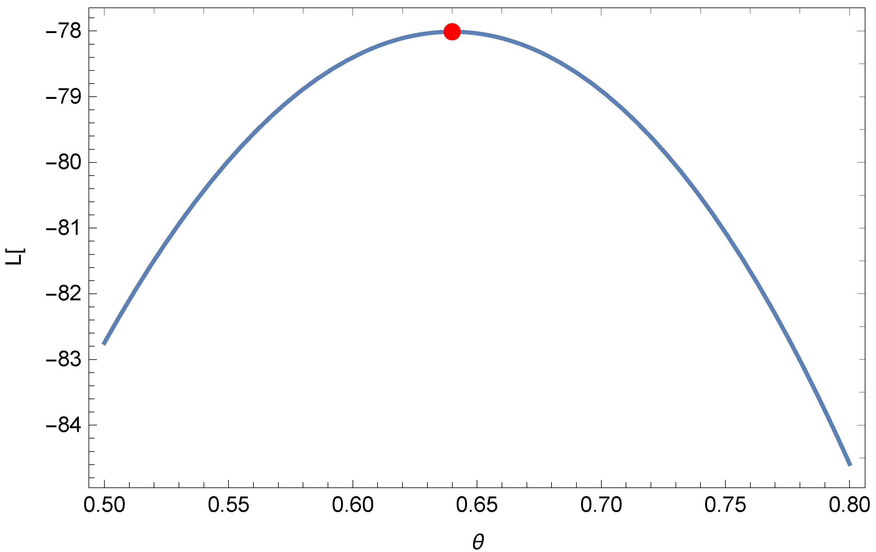
Figure 4 presents the existence and uniqueness of the MLE graphically for this dataset. The goodness-of-fit results are reported in Table 10.
The second dataset represents the minutes of pain relief for 20 patients receiving an analgesic and is taken from [42]. The data are given as follows: 1.1, 1.4, 1.3, 1.7, 1.9, 1.8, 1.6, 2.2, 1.7, 2.7, 4.1, 1.8, 1.5, 1.2, 1.4, 3.0, 1.7, 2.3, 1.6, 2.0. Some descriptive statistics for this dataset are also computed as follows: mean—1.900, median—1.700, standard deviation—0.704, minimum—1.100, maximum—4.100, skewness—1.862, and kurtosis—4.185. 
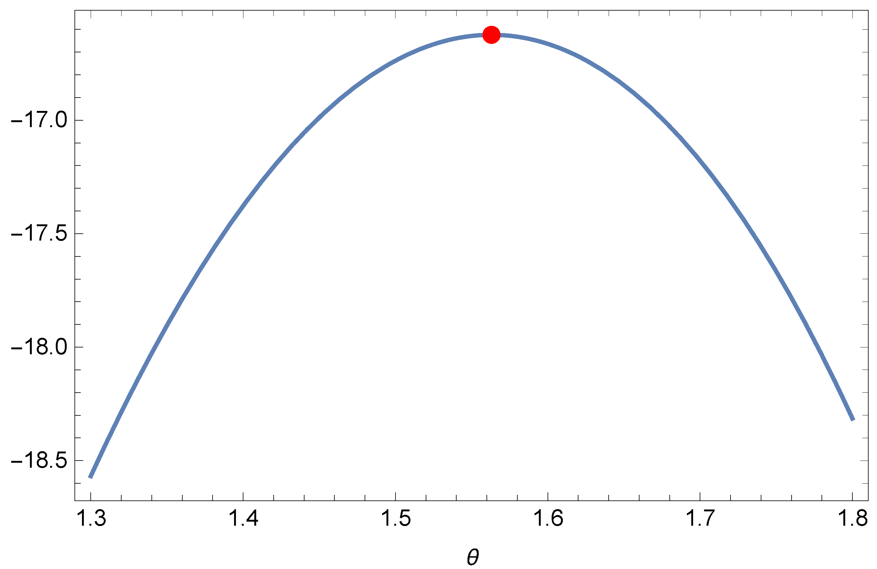
Figure 5 presents the existence and uniqueness of the MLE graphically for this dataset. The goodness-of-fit results are reported in Table 11.
From Table 10 and Table 11, it is easy to conclude that the new distribution gives the best results for all the criteria. Hence, it is quite suitable for modeling datasets related to health. Furthermore, there exists a limited distribution such as the P distribution that can be used to model data within the range of [ 1 , + ) . The novel distribution could serve as a good alternative for such scenarios.
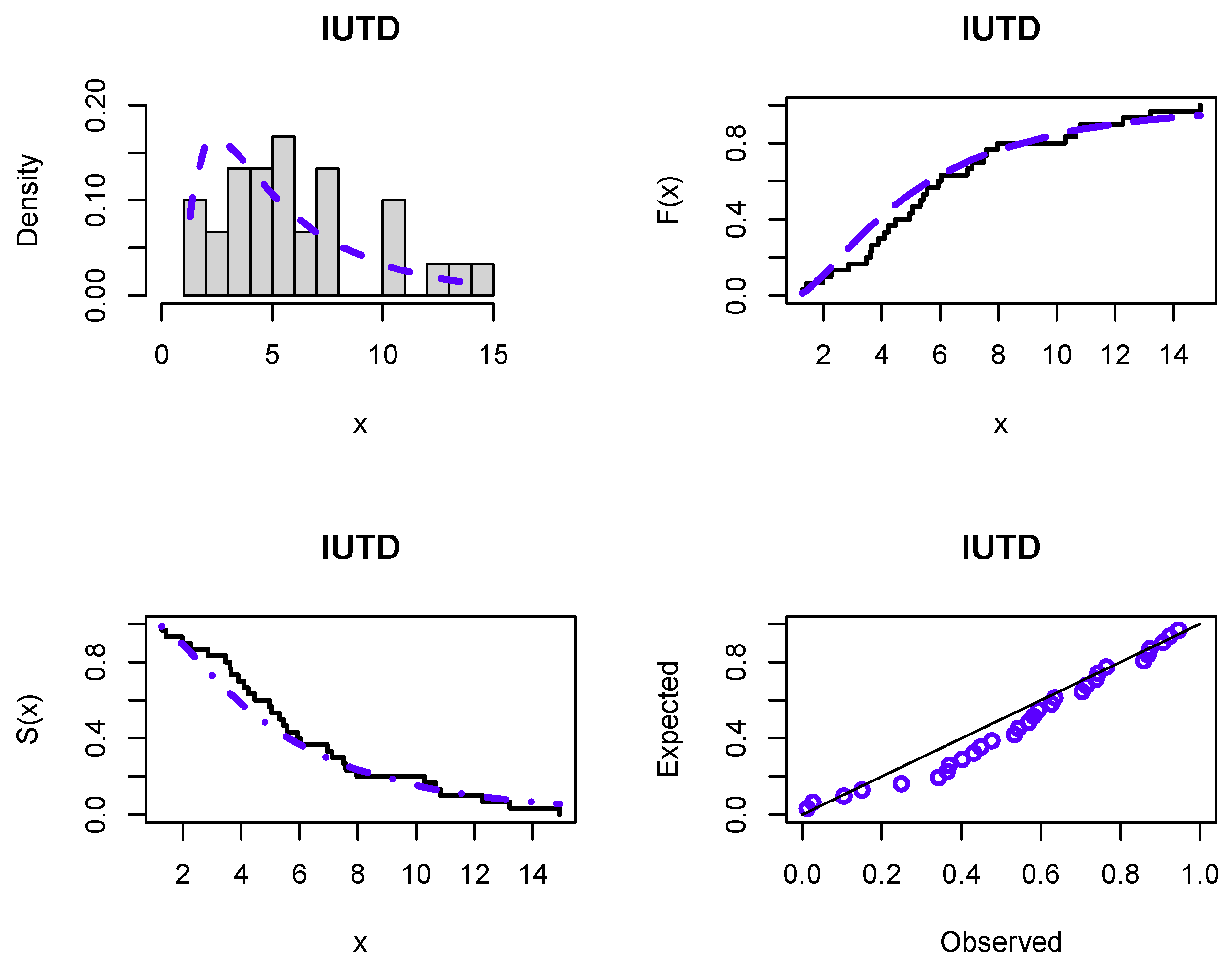
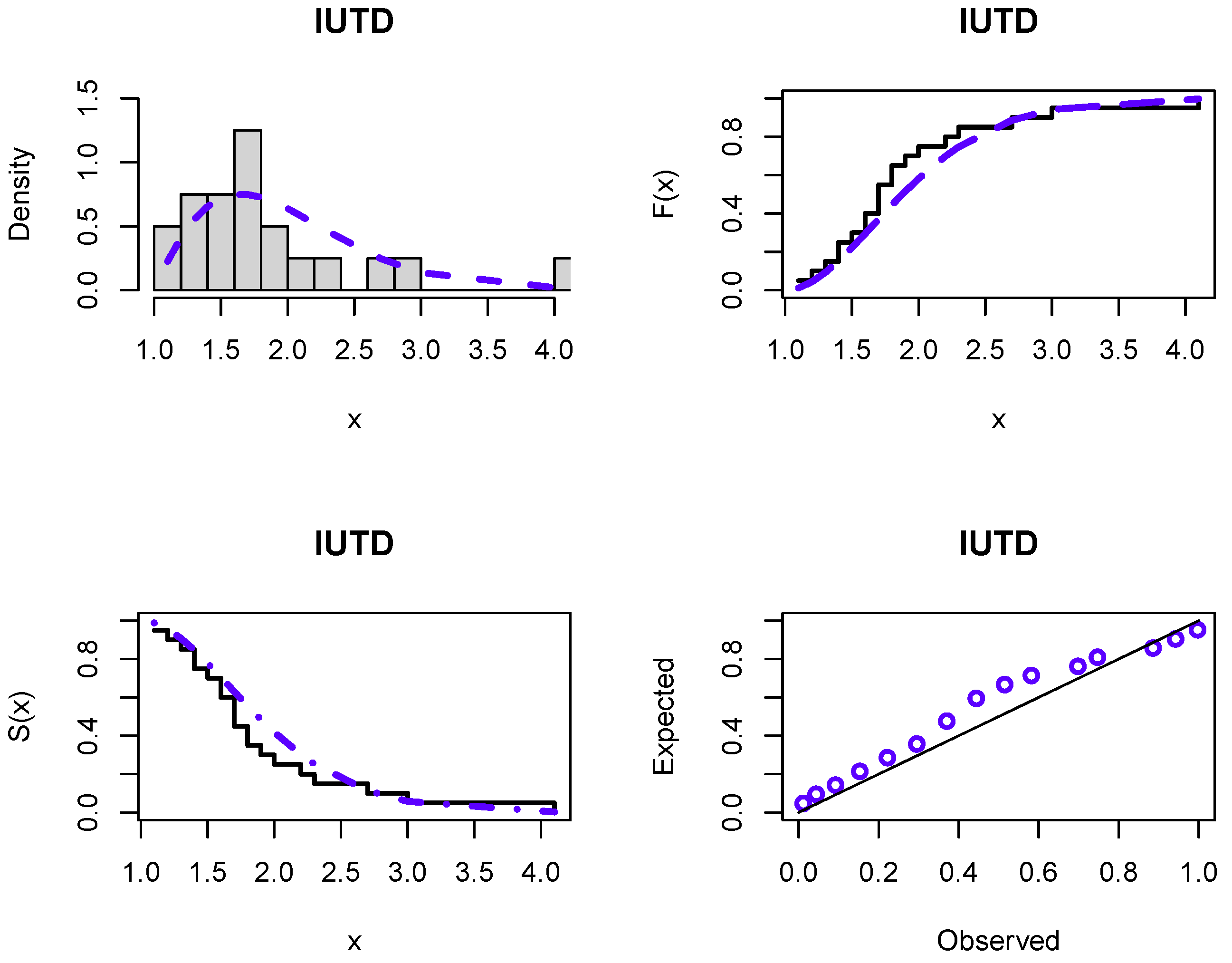
 Figure 6 and Figure 7 display the fitting of the IUTD to both datasets via estimated PDF, CDF, and SF plots, along with probability-probability (P-P) plots. These plots proved that the new distribution is appropriate for both COVID-19 and analgesic datasets.

7. Conclusions

In this paper, we developed a new one-parameter distribution with support as [ 1 , + ) , which can be considered an alternative option to the P distribution. To construct it, the unit Teissier distribution introduced in [14] was utilized as the baseline distribution, and the inversion method was applied. The analysis confirmed that the corresponding PDF exhibits unimodal behavior, and the HRF is observed to be either increasing or unimodal. Some mathematical properties, such as the QF, heavy-tailed nature, stochastic dominance, and incomplete and complete moments, were investigated. In the statistical part, several estimation methods were studied for estimating the unique parameter. The performance of these methods was evaluated through a Monte Carlo simulation, and it was determined that the maximum-likelihood estimation method outperformed the competitors. The Bayesian estimation method using an informative gamma prior distribution under the squared error loss function was discussed. The practical performance of the IUTD is demonstrated via two real datasets. Based on some criteria and goodness-of-fit tests, it exhibits superior performance compared to many inverse and classical distributions, including the P and T distribution.
A natural perspective of this work is the consideration of the distribution of β X , where X is random variable that follows the IUTD and β > 0 , with the following CDF:
F * ( x ) = 1 e 1 ( x / β ) θ x β θ , x β ,
and F * ( x ) = 0 for x < β . We thus relax the lower bound of 1 into the support; it is now of [ β , + ) . Also, all the available extensions of the P distribution can be applied to the IUTD (exponentiated, transmuted, types II, III, IV, etc.). Bivariate and discrete generalizations of the IUTD are also interesting directions for research.

Author Contributions

Conceptualization, N.A., M.E., K.K., A.M.G., C.C. and M.M.A.E.-R.; methodology, N.A., M.E., K.K., A.M.G., C.C. and M.M.A.E.-R.; software, N.A., M.E., K.K., A.M.G., C.C. and M.M.A.E.-R.; validation, N.A., M.E., K.K., A.M.G., C.C. and M.M.A.E.-R.; formal analysis, N.A., M.E., K.K., A.M.G., C.C. and M.M.A.E.-R.; investigation, N.A., M.E., K.K., A.M.G., C.C. and M.M.A.E.-R.; resources, N.A., M.E., K.K., A.M.G., C.C. and M.M.A.E.-R.; data curation, N.A., M.E., K.K., A.M.G., C.C. and M.M.A.E.-R.; writing—original draft preparation, N.A., M.E., K.K., A.M.G., C.C. and M.M.A.E.-R.; writing—review and editing, N.A., M.E., K.K., A.M.G., C.C. and M.M.A.E.-R.; visualization, N.A., M.E., K.K., A.M.G., C.C. and M.M.A.E.-R. All authors have read and agreed to the published version of the manuscript.

Funding

This research was funded by King Saud University, grant number RSPD2023R548.

Data Availability Statement

Not applicable.

Acknowledgments

Researchers Supporting Project number (RSPD2023R548), King Saud University, Riyadh, Saudi Arabia.

Conflicts of Interest

The authors declare no conflict of interest.

References

  1. Alfaer, N.M.; Gemeay, A.M.; Aljohani, H.M.; Afify, A.Z. The Extended Log-Logistic Distribution: Inference and Actuarial Applications. Mathematics 2021, 9, 1386. [Google Scholar] [CrossRef]
  2. Meriem, B.; Gemeay, A.M.; Almetwally, E.M.; Halim, Z.; Alshawarbeh, E.; Abdulrahman, A.T.; Abd El-Raouf, M.M.; Hussam, E. The Power xLindley Distribution: Statistical Inference, Fuzzy Reliability, and COVID-19 Application. J. Funct. Spaces 2022, 2022, 9094078. [Google Scholar] [CrossRef]
  3. Teamah, A.A.M.; Elbanna, A.A.; Gemeay, A.M. Right Truncated Fréchet-Weibull Distribution: Statistical Properties and Application. Delta J. Sci. 2020, 41, 20–29. [Google Scholar] [CrossRef]
  4. Teissier, G. Recherches sur le vieillissement et sur les lois de la mortalité. Ann. Physiol. Physicochim. Biol. 1934, 10, 237–284. [Google Scholar]
  5. Laurent, A.G. Failure and mortality from wear and ageing. The Teissier model. In A Modern Course on Statistical Distributions in Scientific Work: Volume 2—Model Building and Model Selection, Proceedings of the NATO Advanced Study Institute Held at the University of Calgary, Calgary, AB, Canada, 29 July–10 August 1974; Springer: Berlin/Heidelberg, Germany, 1975; pp. 301–320. [Google Scholar]
  6. Muth, E.J. Reliability models with positive memory derived from the mean residual life function. Theory Appl. Reliab. 1977, 2, 401–435. [Google Scholar]
  7. Jodra, P.; Jimenez-Gamero, M.D.; Alba-Fernandez, M.V. On the Muth distribution. Math. Model. Anal. 2015, 20, 291–310. [Google Scholar] [CrossRef]
  8. Jodra, P.; Gomez, H.W.; Jimenez-Gamero, M.D.; Alba-Fernandez, M.V. The power Muth distribution. Math. Model. Anal. 2017, 22, 186–201. [Google Scholar] [CrossRef]
  9. Al-Babtain, A.A.; Elbatal, I.; Chesneau, C.; Jamal, F. The transmuted Muth generated class of distributions with applications. Symmetry 2020, 12, 1677. [Google Scholar] [CrossRef]
  10. Alanzi, A.R.A.; Rafique, M.Q.; Tahir, M.H.; Jamal, F.; Hussain, M.A.; Sami, W. A novel Muth generalized family of distributions: Properties and applications to quality control. AIMS Math. 2023, 8, 6559–6580. [Google Scholar] [CrossRef]
  11. Irshad, M.R.; Maya, R.; Krishna, A. Exponentiated power Muth distribution and associated inference. J. Indian Soc. Probab. Stat. 2021, 22, 265–302. [Google Scholar] [CrossRef]
  12. Chesneau, C.; Agiwal, V. Statistical theory and practice of the inverse power Muth distribution. J. Comput. Math. Data Sci. 2021, 1, 100004. [Google Scholar] [CrossRef]
  13. Almarashi, A.M.; Jamal, F.; Chesneau, C.; Elgarhy, M. A new truncated muth generated family of distributions with applications. Complexity 2021, 2021, 1211526. [Google Scholar] [CrossRef]
  14. Krishna, A.; Maya, R.; Chesneau, C.; Irshad, M.R. The Unit Teissier Distribution and Its Applications. Math. Comput. Appl. 2022, 27, 12. [Google Scholar] [CrossRef]
  15. Bernardo, J.M.; Smith, A.F.M. Bayesian Theory; Wiley: New York, NY, USA, 1994; Volume 49. [Google Scholar]
  16. Sharma, V.K.; Singh, S.K.; Singh, U.; Agiwal, V. The inverse Lindley distribution: A stress-strength reliability model with application to head and neck cancer data. J. Ind. Prod. Eng. 2015, 32, 162–173. [Google Scholar] [CrossRef]
  17. Yadav, A.S.; Maiti, S.S.; Saha, M. The inverse xgamma distribution: Statistical properties and different methods of estimation. Ann. Data Sci. 2021, 8, 275–293. [Google Scholar] [CrossRef]
  18. Barco, K.V.P.; Mazucheli, J.; Janeiro, V. The inverse power Lindley distribution. Commun. Stat.-Simul. Comput. 2017, 46, 6308–6323. [Google Scholar] [CrossRef]
  19. Abd AL-Fattah, A.M.; El-Helbawy, A.A.; Al-Dayian, G.R. Inverted kumaraswamy distribution: Properties and estimation. Pak. J. Stat. 2017, 33, 37–61. [Google Scholar]
  20. Lee, S.; Noh, Y.; Chung, Y. Inverted exponentiated Weibull distribution with applications to lifetime data. Commun. Stat. Appl. Methods 2017, 24, 227–240. [Google Scholar] [CrossRef]
  21. Hassan, A.S.; Nassr, S.G. The inverse weibull generator of distributions: Properties and applications. J. Data Sci. 2018, 16, 723–742. [Google Scholar] [CrossRef]
  22. Tahir, M.H.; Cordeiro, G.M.; Ali, S.; Dey, S.; Manzoor, A. The inverted Nadarajah–Haghighi distribution: Estimation methods and applications. J. Stat. Comput. Simul. 2018, 88, 2775–2798. [Google Scholar] [CrossRef]
  23. Hassan, A.S.; Abd-Allah, M. On the inverse power Lomax distribution. Ann. Data Sci. 2019, 6, 259–278. [Google Scholar] [CrossRef]
  24. Hassan, A.S.; Elgarhy, M.; Ragab, R. Statistical properties and estimation of inverted Topp-Leone distribution. J. Stat. Appl. Probab. 2020, 9, 319–331. [Google Scholar]
  25. Omar, M.H.; Arafat, S.Y.; Hossain, M.P.; Riaz, M. Inverse maxwell distribution and statistical process control: An efficient approach for monitoring positively skewed process. Symmetry 2021, 13, 189. [Google Scholar] [CrossRef]
  26. Louzada, F.; Ramos, P.L.; Nascimento, D. The inverse Nakagami-m distribution: A novel approach in reliability. IEEE Trans. Reliab. 2018, 67, 1030–1042. [Google Scholar] [CrossRef]
  27. Guo, L.; Gui, W. Bayesian and classical estimation of the inverse Pareto distribution and its application to strength-stress models. Am. J. Math. Manag. Sci. 2018, 37, 80–92. [Google Scholar] [CrossRef]
  28. Clauset, A.; Shalizi, C.R.; Newman, M.E.J. Power-law distributions in empirical data. SIAM Rev. 2009, 51, 661–703. [Google Scholar] [CrossRef]
  29. Mitzenmacher, M. A Brief History of Generative Models for Power Law and Lognormal Distributions. Internet Math. 2003, 1, 226–251. [Google Scholar] [CrossRef]
  30. Johnson, N.L.; Kotz, S.; Balakrishnan, N. Continuous Univariate Distributions; John Wiley & Sons: New York, NY, USA, 1995; Volume 2. [Google Scholar]
  31. Belzunce, F.; Riquelme, C.M.; Mulero, J. An Introduction to Stochastic Orders; Academic Press: Cambridge, MA, USA, 2015. [Google Scholar]
  32. Anderson, T.W.; Darling, D.A. Asymptotic theory of certain “goodness of fit” criteria based on stochastic processes. Ann. Math. Stat. 1952, 23, 193–212. [Google Scholar] [CrossRef]
  33. Mukhtar, M.S.; El-Morshedy, M.; Eliwa, M.S.; Yousof, H.M. Expanded Fréchet model: Mathematical properties, copula, different estimation methods, applications and validation testing. Mathematics 2020, 8, 1949. [Google Scholar]
  34. Choi, K.; Bulgren, W.G. An estimation procedure for mixtures of distributions. J. R. Stat. Soc. Ser. B (Methodol.) 1968, 30, 444–460. [Google Scholar] [CrossRef]
  35. Swain, J.J.; Venkatraman, S.; Wilson, J.R. Least-squares estimation of distribution functions in Johnson’s translation system. J. Stat. Comput. Simul. 1988, 29, 271–297. [Google Scholar] [CrossRef]
  36. Kao, J.H.K. Computer methods for estimating Weibull parameters in reliability studies. IRE Trans. Reliab. Qual. Control 1958, PGRQC-13, 15–22. [Google Scholar] [CrossRef]
  37. Torabi, H. A general method for estimating and hypotheses testing using spacings. J. Stat. Theory Appl. 2008, 8, 163–168. [Google Scholar]
  38. R Core Team. R: A Language and Environment for Statistical Computing; R Foundation for Statistical Computing: Vienna, Austria, 2013. [Google Scholar]
  39. Chen, M.H.; Shao, Q.M. Monte Carlo Estimation of Bayesian Credible and HPD Intervals. J. Comput. Graph. Stat. 1999, 8, 69–92. [Google Scholar]
  40. Almongy, H.M.; Almetwally, E.M.; Aljohani, H.M.; Alghamdi, A.S.; Hafez, E.H. A new extended Rayleigh distribution with applications of COVID-19 data. Results Phys. 2021, 23, 104012. [Google Scholar] [CrossRef] [PubMed]
  41. Arif, M.; Khan, D.M.; Aamir, M.; Khalil, U.; Bantan, R.A.R.; Elgarhy, M. Modeling COVID-19 data with a novel extended exponentiated class of distributions. J. Math. 2022, 2022, 1908161. [Google Scholar] [CrossRef]
  42. Gross, A.J.; Clark, V.A. Survival Distributions: Reliability Applications in the Biomedical Sciences; Wiley: New York, NY, USA, 1975; Volume 11. [Google Scholar]
Figure 1. Plots of the PDF of the IUTD.
Axioms 12 00502 g001
Figure 2. Plots of the HRF of the IUTD.
Axioms 12 00502 g002
Figure 3. Distribution and convergence of the MCMC estimates for θ utilizing the MH algorithm at θ = 0.75 and n = 40 .
Axioms 12 00502 g003
Figure 4. Plot of the profile-likelihood function for the first dataset with the unique maximum indicated by a red dot.
Axioms 12 00502 g004
Figure 5. Plot of the profile-likelihood function for the second dataset with the unique maximum indicated by a red dot.
Axioms 12 00502 g005
Figure 6. The histogram of the first dataset with the fitted PDF in blue, as well as the fitted CDF, SF, and P-P plots in blue too.
Axioms 12 00502 g006
Figure 7. The histogram of the second dataset with the fitted PDF in blue, as well as the fitted CDF, SF, and P-P plots in blue too.
Axioms 12 00502 g007
Table 1. Some numerical values of crucial measures for the IUTD.
Measure θ
0.10.30.81.01.52.02.54.05.0
M * 2.885442.855322.205462.01.681511.510221.4061.25021.19891
Q ( 0.25 ) 0.01304870.05542570.3379810.4198690.5607150.6479730.7067170.8049680.840664
Q ( 0.5 ) 0.0006710.00766860.1609790.2319610.3775230.4816230.5573990.6939910.746591
Q ( 0.75 ) 0.000010.0004930570.05752230.1018280.2180620.3191060.4010030.5648940.633248
SK−0.89866−0.738751−0.262233−0.18166−0.0692568−0.01165170.02315140.07547590.0929066
KU4.31042.419051.203551.15411.131941.141981.155451.186921.20057
Table 8. Numerical values of the Bayesian estimation for the IUTD.
n204060100120200
θ = 0.75
Mean0.776440.736690.746020.753050.745620.75114
MSE0.001060.000650.000530.000470.000230.00012
RMSE0.032500.025450.023110.021700.015300.01073
θ = 1.0
Mean1.013170.995161.015041.001830.995041.01427
MSE0.000980.000970.000940.000610.000610.00058
RMSE0.031270.031110.030590.024760.024730.02406
θ = 2.5
Mean2.542912.464582.487062.505692.491622.48585
MSE0.016950.007090.005140.002080.001370.00136
RMSE0.130210.084210.071680.045610.036980.03691
θ = 4.0
Mean4.111744.035413.963893.959444.055913.97469
MSE0.048130.017620.014430.011420.009550.00767
RMSE0.219380.132720.120110.106840.097740.08761
θ = 6.0
Mean5.940626.116896.098716.004016.009036.01019
MSE0.054440.052550.030000.017600.015350.01308
RMSE0.233330.229240.173210.132650.123890.11437
θ = 10.0
Mean10.1127210.0572510.0619610.1332210.083509.99554
MSE0.223970.192660.097580.078960.066350.03698
RMSE0.473250.438930.312370.280990.257590.19229
θ = 12.0
Mean11.8495912.0242112.1085311.9352712.1148512.07960
MSE0.188260.130270.073880.071910.061060.02722
RMSE0.433890.360930.271810.268150.247110.16499
Table 9. List of the PDFs for the considered distributions, with θ > 0 representing the only one common parameter.
DistributionPDFSupport
IUTD θ e 1 x θ x θ 1 x θ 1 [ 1 , + )
P θ x 1 + θ [ 1 , + )
T θ e θ x 1 e θ x e θ x + 1 [ 0 , + )
E 1 θ e x / θ [ 0 , + )
Li x + 1 θ 2 1 + θ e θ x [ 0 , + )
IL x + 1 θ 2 1 + θ x 3 e θ / x ( 0 , + )
IP θ x θ 1 x + 1 1 + θ ( 0 , + )
IR 2 θ e θ / x 2 x 3 ( 0 , + )
IXG θ 2 1 + θ / ( 2 x 2 ) e θ / x 1 + θ x 2 ( 0 , + )
Table 10. The goodness-of-fit results for the first dataset.
IUTPTELiILIPIRIXG
^ −78.0117−94.3841−79.5285−84.5253−79.9640−85.2373−87.1103−83.2789−86.2698
AIC158.0234190.7682161.0571171.0505161.9281172.4747176.2206168.5577174.5396
BIC159.4246192.1694162.4583172.4517163.3292173.8759177.6218169.9589175.9408
CAIC158.1663190.9111161.1999171.1934162.0709172.6175176.3634168.7006174.6824
HQIC158.4717191.2165161.5053171.4988162.3763172.9229176.6688169.0060174.9878
KS0.17560.36270.22030.26340.17940.24280.27340.21780.2620
AD0.84705.27272.00912.70761.06262.38213.12612.38602.8035
CVM0.16811.07360.39570.50030.17040.42210.58280.45210.5140
KS p-val0.27920.00050.09290.02520.25690.04830.01800.09940.0263
AD p-val0.44730.00220.09120.03900.32540.05760.02390.05730.0348
CVM p-val0.34010.00140.07360.03910.33410.06250.02400.05210.0360
θ 0.64000.60710.14626.15650.28854.95954.922011.84885.5032
se of θ 0.04520.11080.01011.12400.03770.79190.89862.16330.8718
Table 11. The goodness-of-fit results for the second dataset.
IUTPTELiILIPIRIXG
^ −16.6238−21.2071−21.8751−32.8371−30.2495−31.7572−36.7278−21.1825−33.6363
AIC35.247644.414345.750167.674262.499165.514475.455744.365069.2727
BIC36.243345.410046.745968.669963.494866.510176.451445.360770.2684
CAIC35.469844.636545.972467.896462.721365.736675.677944.587269.4949
HQIC35.442044.608745.944567.868562.693565.708875.650044.559469.4670
KS0.20580.28500.19210.43950.39110.36950.42090.25660.4038
AD0.86182.17581.34174.60353.75044.46895.49222.06545.0874
CVM0.16880.42540.22630.96300.75500.90541.14550.39761.0562
KS p-val0.36540.07750.45160.00090.00440.00850.00170.14360.0029
AD p-val0.43700.07430.21910.00460.01180.00530.00170.08520.0027
CVM p-val0.33900.06100.22240.00260.00860.00360.00090.07240.0015
θ 1.56311.69710.53561.90000.81612.25472.21252.76072.7245
se of θ 0.13150.37950.04530.42490.13610.40890.49470.61730.4855
Disclaimer/Publisher’s Note: The statements, opinions and data contained in all publications are solely those of the individual author(s) and contributor(s) and not of MDPI and/or the editor(s). MDPI and/or the editor(s) disclaim responsibility for any injury to people or property resulting from any ideas, methods, instructions or products referred to in the content.

