The Multivariable Zhang–Zhang Polynomial of Phenylenes

Abstract

The Zhang–Zhang polynomial of a benzenoid system is a well-known counting polynomial that was introduced in 1996. It was designed to enumerate Clar covers, which are spanning subgraphs with only hexagons and edges as connected components. In 2018, the generalized Zhang–Zhang polynomial of two variables was defined such that it also takes into account 10-cycles of a benzenoid system. The aim of this paper is to introduce and study a new variation of the Zhang–Zhang polynomial for phenylenes, which are important molecular graphs composed of 6-membered and 4-membered rings. In our case, Clar covers can contain 4-cycles, 6-cycles, 8-cycles, and edges. Since this new polynomial has three variables, we call it the multivariable Zhang–Zhang (MZZ) polynomial. In the main part of the paper, some recursive formulas for calculating the MZZ polynomial from subgraphs of a given phenylene are developed and an algorithm for phenylene chains is deduced. Interestingly, computing the MZZ polynomial of a phenylene chain requires some techniques that are different to those used to calculate the (generalized) Zhang–Zhang polynomial of benzenoid chains. Finally, we prove a result that enables us to find the MZZ polynomial of a phenylene with branched hexagons.

1. Introduction

Kekulé structures are often employed to provide an insight into the $\pi$-electron structure of polycyclic conjugated molecules (note that a Kekulé structure of a polycyclic conjugated hydrocarbon is represented by a structural formula with double bonds between certain pairs of carbon atoms, such that each carbon atom is adjacent to exactly one double bond). When a molecule is modelled by the molecular graph, Kekulé structures are in one-to-one correspondence with the perfect matchings of the obtained graph [1,2]. Since Kekulé structures can be used to predict various properties and chemical behaviour of molecules [2,3], the investigation and enumeration of these structures is a classical topic in theoretical and mathematical chemistry.

A theory closely related to the concept of Kekulé structures is the Clar’s aromatic sextet theory [4]. In accordance with this theory, H. Zhang and F. Zhang introduced the concept of Clar covers [5]. Note that a Clar cover of a benzenoid system (i.e., a benzenoid graph that can be embedded into the regular hexagonal lattice) consists of some hexagons (which represent the aromatic sextets) and of double bonds such that all vertices of the graph are covered. The maximum possible number of hexagons among all Clar covers in a given benzenoid graph is known as the Clar number. By Clar’s theory, the most important Kekulé structures are those in which the number of aromatic sextets equals the Clar number. Some well-investigated concepts that are closely related to Clar covers are resonant sets, alternating sets, and the Fries number (for some research on these topics see [6,7,8,9]).

In [5], the authors also introduced the so called Clar covering polynomial that was later named the Zhang–Zhang polynomial. For a benzenoid system G, this polynomial is defined as

$$ZZ(G;x)=\sum _{p\ge 0}z(G;p)x^p,$$

where $z(G;p)$ is the number of Clar covers of G with exactly p hexagons. It is interesting that the Clar number, the number of Kekulé structures, and the first Herndon number can be easily calculated by using this polynomial. For some recent papers on the Zhang–Zhang polynomial, see [10,11,12].

Another topic closely related to the above-mentioned concepts is the study of resonance graphs. These graphs are used to model interactions among different Kekulé structures; see [13] for a survey on this topic. It is worth mentioning that the relation between the Zhang–Zhang polynomial of a molecular graph and the cube polynomial of its resonance graph was considered for different families of graphs [12,14]. Some recent research on resonance graphs can be found, for example, in [15].

In [16], the generalized Zhang–Zhang polynomial (GZZ polynomial) was introduced in order to increase the sensibility of the standard Zhang–Zhang polynomial. This polynomial contains two variables and counts so-called generalized Clar covers, which can contain edges, hexagons, and also 10-cycles (representing two adjacent hexagons). Therefore, the GZZ polynomial gives explicit information on $\pi$-electron cyclic conjugation within 10-membered rings. It was shown in the same paper that for some families of molecular graphs, the GZZ polynomial of a given graph is equal to the generalized cube polynomial of the corresponding resonance graph. Later, several recursive formulas for calculating the GZZ polynomial of benzenoid systems were derived and numerical results were obtained in order to test the relation between the GZZ polynomial and three energy-based quantities [17]. Furthermore, it was shown that the molecular vibrational energies can be related to Clar-structure-based parameters by using the GZZ polynomial [18].

The aim of this paper is to introduce another variant of the Zhang–Zhang polynomial for phenylenes. Note that phenylenes are conjugated systems composed of 6-membered rings and 4-membered rings and, therefore, the $\pi$-electron properties of these molecules are of great interest for theoretical chemistry. For some results related to the Kekulé structures of phenylenes, see [19,20,21], and more information on the chemistry of phenylenes can be found in the references stated in [20]. In order to take into account 4-membered rings, 6-membered rings, and also combinations of these rings, the corresponding Clar covers should not contain only 6-cycles (hexagons) and edges, but also 4-cycles (quadrilaterals) and 8-cycles. Hence, our new polynomial has three variables; therefore, we call it the multivariable Zhang–Zhang polynomial (in short, the MZZ polynomial). It is clear that this polynomial provides some information on the distribution of $\pi$-electrons in phenylenes. Moreover, as we already mentioned, such approach could have interesting chemical applications [17,18].

In the next section, we state some basic definitions and formally introduce the MZZ polynomial. Next, in Section 3, we prove several recursive formulas that enable use to calculate the MZZ polynomial of a phenylene by using the MZZ polynomials of its subgraphs. An efficient algorithm for computing the MZZ polynomial of any phenylene chain is then deduced in Section 4. Finally, in Section 5 we discuss how to calculate the MZZ polynomial of a phenylene with branched hexagons.

2. Preliminaries

In this paper, we consider only finite and simple graphs. For a graph G, we denote by $V\left(G\right)$ the set of vertices and by $E\left(G\right)$ the set of edges of G. The degree of a vertex $v\in V\left(G\right)$ is the number of vertices adjacent to v. If $k\ge 3$, then a cycle of length k in G, denoted as $C_k$, will be called a k-cycle of G.

Let G be a plane graph. Two distinct faces of G are adjacent if they share a common edge. We denote the set of edges lying on some face f of G by $E\left(f\right)$. Also, the subgraph induced by the edges in $E\left(f\right)$ is the boundary of f. An inner face of G whose boundary is a 6-cycle $C_6$ is called a hexagon of G. Similarly, an inner face of G whose boundary is a 4-cycle $C_4$ is called a quadrilateral of G. Furthermore, the vertices of G that belong to the outer face are known as boundary vertices and all the other vertices of G are interior vertices. Similarly, the edges lying on the outer face will be called boundary edges. An outerplane graph is a plane graph in which all vertices are boundary vertices.

A benzenoid graph is a bipartite 2-connected plane graph in which all interior vertices have degree 3, all boundary vertices have degree 2 or 3, and all inner faces are hexagons. It is worth mentioning that these graphs are sometimes referred to as fusenes [22]. Note also that by our definition, a benzenoid graph is not always a subgraph of the regular hexagonal lattice. Moreover, a benzenoid graph which does not contain any interior vertices (i.e., an outerplane benzenoid graph) is called a catacondensed benzenoid graph.

Let B be a catacondensed benzenoid graph. If we add a quadrilateral between any two adjacent hexagons of B, then the obtained graph is called a phenylene. In Figure 1, we can see a catacondensed benzenoid graph B and the corresponding phenylene G.

To deduce our main results of the paper, we need to consider a wider family of graphs and not just phenylenes. Therefore, throughout the paper a generalized phenylene will be an outerplane bipartite graph in which no two distinct quadrilaterals are adjacent. It is easy to check that in such a graph every 4-cycle is the boundary of some quadrilateral, every 6-cycle is the boundary of some hexagon, and in the interior of every 8-cycle there is either one inner face or one quadrilateral and one hexagon (with the common edge).

Let h be a hexagon of a generalized phenylene G such that h contains exactly two vertices of degree 2, which will be denoted as x and y. We say that h is angular if $xy$ is an edge of G, and on the other hand, h is linear if x and y are not adjacent in G. Moreover, if G is a phenylene, then a hexagon of G is called branched if it is adjacent to exactly three quadrilaterals of G. It is easy to see that phenylene G from Figure 1 contains two angular hexagons, one linear hexagon, and no branched hexagons. On the other hand, a phenylene from Figure 2 contains one angular hexagon, two linear hexagons, and one branched hexagon.

Let G be a phenylene. If every hexagon of G is adjacent to at most two quadrilaterals, we say that G is a phenylene chain. In addition, a linear phenylene chain is a phenylene chain that does not contain any angular hexagons. Obviously, phenylene G from Figure 1 is a phenylene chain, but G is not a linear phenylene chain.

A subset of edges M of a graph G is called a perfect matching of G if every vertex of G is an end vertex of exactly one edge from M. It is well known that in chemistry, perfect matchings are usually referred to as Kekulé structures.

A spanning subgraph C of a generalized phenylene G is a (4,6,8)-Clar cover of G if every connected component of C is a 4-cycle $C_4$ (a quadrilateral), a 6-cycle $C_6$ (a hexagon), an 8-cycle $C_8$, or an edge $K_2$. Figure 2 shows a phenylene with a (4,6,8)-Clar cover composed of one 8-cycle, two hexagons, two quadrilaterals, and seven edges (the bold edges in the figure represent connected components of this (4,6,8)-Clar cover).

Finally, we introduce the multivariable Zhang–Zhang polynomial (or shortly MZZ polynomial) $MZZ(G;x,y,z)$ of a generalized phenylene G by setting

$$MZZ(G;x,y,z)=\sum _{p,q,r\ge 0}mz(G;p,q,r)x^p{y}^q{z}^r,$$

where $mz(G;p,q,r)$ represents the number of (4,6,8)-Clar covers of G that contain exactly p quadrilaterals, q hexagons, and r 8-cycles. Moreover, if G has no vertices, we consider the set ∅ as the unique (4,6,8)-Clar cover of G, so in this case we define $MZZ(G;x,y,z)=1$. Furthermore, the MZZ polynomial of G will be often denoted simply as $MZZ\left(G\right)$, i.e., $MZZ\left(G\right):=MZZ(G;x,y,z)$.

Some simple observations about the $MZZ$ polynomial of a generalized phenylene G can now be stated:

 $\left(i\right)$

The number of perfect matchings of G is exactly $mz(G;0,0,0)$, which is equal to $MZZ(G;0,0,0)$. Therefore, the number of perfect matchings can be obtained by taking $x=y=z=0$ into the MZZ polynomial.

$\left(ii\right)$

If G does not have any perfect matching, then the set of all (4,6,8)-Clar covers of G is empty, so $MZZ\left(G\right)=0$.

$\left(iii\right)$

If G has only one perfect matching, then G has exactly one (4,6,8)-Clar cover which contains only edges from the unique perfect matching, so $MZZ\left(G\right)=1$.

$\left(iv\right)$

It can be observed that if G is a phenylene, then the set of all hexagons of G is always a (4,6,8)-Clar cover of G (which contains only hexagons as connected components). Therefore, the MZZ polynomial of a phenylene with $h\left(G\right)$ hexagons always contains the term $y^{h\left(G\right)}$.

Suppose that G is a generalized phenylene and let $\mathbb{CC}\left(G\right)$ be the set of all (4,6,8)-Clar covers of G. In addition, for any $C\in \mathbb{CC}\left(G\right)$ let $q\left(C\right)$ be the number of quadrilaterals of C, $h\left(C\right)$ the number of hexagons of C, and $o\left(C\right)$ as the number of 8-cycles of C. It is not difficult to see that we can express the $MZZ$ polynomial in the following way.

Proposition 1.

If G is a generalized phenylene, then

$$MZZ\left(G\right)=\sum _{C\in \mathbb{CC}\left(G\right)}{x}^{q\left(C\right)}{y}^{h\left(C\right)}{z}^{o\left(C\right)}.$$

Note that if $\mathbb{CC}\left(G\right)=\varnothing$ in the above proposition, then the index set of the corresponding sum is empty, so $MZZ\left(G\right)=0$.

We finish this section with one additional notation. If G is a generalized phenylene, C a (4,6,8)-Clar cover of G, and H a quadrilateral, a hexagon, an 8-cycle, or an edge of G, then by writing $H\in C$ we mean that H is a connected component of C.

3. Computing the MZZ Polynomial from Smaller Graphs

In this section, we provide several results that enable us to calculate the MZZ polynomial of a generalized phenylene by using the MZZ polynomials of subgraphs of the original graph. We should mention that the results stated in this section are analogous to those from [5,17], but several additional insights are needed in our case.

The following notation will be used for any generalized phenylene G:

• If $e=uv$ is an edge of G, then $G-e=G-uv$ denotes the graph obtain from G by deleting edge e;
• If $e=uv$ is an edge of G, then $G-u-v$ denotes the graph obtain from G by deleting vertices u and v, together with all the edges incident to u or v;
• If f is an inner face of G, then $G-f$ denotes the graph obtain from G by deleting all the vertices of f, together with all the edges incident to the vertices of f;
• If f and $f^{\prime }$ are two adjacent inner faces of G, then $G-f-f^{\prime }$ denotes the graph obtain from G by deleting all the vertices of f and all the vertices of $f^{\prime }$, together with all the edges incident to these vertices;
• If f is a hexagon of G and $f^{\prime }$ a quadrilateral of G such that f and $f^{\prime }$ are adjacent, then $f{f}^{\prime }$ denotes the unique 8-cycle of G induced by f and $f^{\prime }$.

In the first theorem we show that the MZZ polynomial of a generalized phenylene G is equal to the product of MZZ polynomials of connected components of G.

Theorem 1.

Let G be a generalized phenylene with connected components $G_1,G_2,\dots ,G_p$. Then it holds

$$MZZ\left(G\right)=\prod _{j=1}^{p}MZZ\left(G_j\right).$$

Proof. 

If $\mathbb{CC}\left(G\right)=\varnothing$, the result is obvious. Otherwise, we can write the set $\mathbb{CC}\left(G_j\right)$ as $\mathbb{CC}\left(G_j\right)=\{C{|}_{G_j}:C\in \mathbb{CC}\left(G\right)\}$, where ${C|}_{G_j}$ denotes the restriction of C to $G_j$ for any $j\in \{1,\dots ,p\}$. Therefore, one can obtain

$$\begin{array}{ccc}\hfill MZZ\left(G\right)& =& \sum _{C\in \mathbb{CC}\left(G\right)}{x}^{q\left(C\right)}{y}^{h\left(C\right)}{z}^{o\left(C\right)}=\sum _{C\in \mathbb{CC}\left(G\right)}\prod _{j=1}^p{x}^{q\left(C{|}_{G_j}\right)}{y}^{h\left(C{|}_{G_j}\right)}{z}^{o\left(C{|}_{G_j}\right)}\hfill \\ & =& \sum _{C^1\in \mathbb{CC}\left(G_1\right)}\sum _{C^2\in \mathbb{CC}\left(G_2\right)}\cdots \sum _{C^p\in \mathbb{CC}\left(G_p\right)}\prod _{j=1}^p{x}^{q\left(C^j\right)}{y}^{h\left(C^j\right)}{z}^{o\left(C^j\right)}\hfill \\ & =& \prod _{j=1}^p\sum _{C^j\in \mathbb{CC}\left(G_j\right)}{x}^{q\left(C^j\right)}{y}^{h\left(C^j\right)}{z}^{o\left(C^j\right)}=\prod _{j=1}^{p}MZZ\left(G_j\right),\hfill \end{array}$$

which is the desired result.    □

The next theorem can be applied when one has a generalized phenylene composed of several generalized phenylenes joined by edges.

Theorem 2.

If G is a generalized phenylene and $e=uv$ is an edge of G not belonging to any quadrilateral, hexagon or 8-cycle of G, then it holds

$$MZZ\left(G\right)=MZZ(G-u-v)+MZZ(G-e).$$

Proof. 

If $\mathbb{CC}\left(G\right)=\varnothing$, the result obviously follows. Therefore, we can suppose $\mathbb{CC}\left(G\right)\ne \varnothing$. Let ${\mathbb{CC}}^1=\{C\in \mathbb{CC}\left(G\right):e\in C\}$ and ${\mathbb{CC}}^2=\{C\in \mathbb{CC}\left(G\right):e\notin C\}$. Therefore, we obtain

$$\begin{array}{ccc}\hfill MZZ\left(G\right)& =& \sum _{C\in \mathbb{CC}\left(G\right)}{x}^{q\left(C\right)}{y}^{h\left(C\right)}{z}^{o\left(C\right)}\hfill \\ & =& \sum _{C\in {\mathbb{CC}}^1}{x}^{q\left(C\right)}{y}^{h\left(C\right)}{z}^{o\left(C\right)}+\sum _{C\in {\mathbb{CC}}^2}{x}^{q\left(C\right)}{y}^{h\left(C\right)}{z}^{o\left(C\right)}\hfill \\ & =& \sum _{C\in {\mathbb{CC}}^1}{x}^{q(C-e)}{y}^{h(C-e)}{z}^{o(C-e)}+\sum _{C\in {\mathbb{CC}}^2}{x}^{q\left(C\right)}{y}^{h\left(C\right)}{z}^{o\left(C\right)}.\hfill \end{array}$$

We can easily see that

$$\sum _{C\in {\mathbb{CC}}^1}{x}^{q(C-e)}{y}^{h(C-e)}{z}^{o(C-e)}=\sum _{C\in \mathbb{CC}(G-u-v)}{x}^{q\left(C\right)}{y}^{h\left(C\right)}{z}^{o\left(C\right)}.$$

On the other hand, we know that e does not belong to any quadrilateral, hexagon or 8-cycle of G, which implies

$$\sum _{C\in {\mathbb{CC}}^2}{x}^{q\left(C\right)}{y}^{h\left(C\right)}{z}^{o\left(C\right)}=\sum _{C\in \mathbb{CC}(G-e)}{x}^{q\left(C\right)}{y}^{h\left(C\right)}{z}^{o\left(C\right)}.$$

Therefore, we obtain

$$\begin{array}{ccc}\hfill MZZ\left(G\right)& =& \sum _{C\in \mathbb{CC}(G-u-v)}{x}^{q\left(C\right)}{y}^{h\left(C\right)}{z}^{o\left(C\right)}+\sum _{C\in \mathbb{CC}(G-e)}{x}^{q\left(C\right)}{y}^{h\left(C\right)}{z}^{o\left(C\right)}\hfill \\ & =& MZZ(G-u-v)+MZZ(G-e),\hfill \end{array}$$

which completes the proof.    □

The following theorem will be essentially used in the proofs of some other results.

Theorem 3.

Suppose that G is a generalized phenylene. Let $e=uv$ be a boundary edge of G such that e also lies on some hexagon f of G (see Figure 3). Also, let $p\le 5$ denotes the number of quadrilaterals adjacent to f. If $p=0$, then

$$MZZ\left(G\right)=yMZZ(G-f)+MZZ(G-u-v)+MZZ(G-e).$$

If $p\ne 0$, let $f_1,\dots ,f_p$ be the quadrilaterals adjacent to f. Then

$$\begin{array}{ccc}\hfill MZZ\left(G\right)& =& yMZZ(G-f)+MZZ(G-u-v)\hfill \\ & +& z\sum _{j=1}^{p}MZZ(G-f-f_j)+MZZ(G-e).\hfill \end{array}$$

Proof. 

If $\mathbb{CC}\left(G\right)=\varnothing$, the result obviously follows. Therefore, assume $\mathbb{CC}\left(G\right)\ne \varnothing$. Note that the details of the proof will be stated only for $p\ne 0$, since the case $p=0$ is easier. Firstly, we introduce the following sets:

$$\begin{array}{ccc}\hfill {\mathbb{CC}}^1& =& \{C\in \mathbb{CC}(G):f\in C\},\hfill \\ \hfill {\mathbb{CC}}^2& =& \{C\in \mathbb{CC}(G):e\in C\},\hfill \\ \hfill {\mathbb{CC}}^{3j}& =& \{C\in \mathbb{CC}\left(G\right):f{f}_j\in C\}\mathrm{for}j\in \{1,\dots ,p\},\hfill \\ \hfill {\mathbb{CC}}^4& =& \mathbb{CC}\left(G\right)-{\mathbb{CC}}^1-{\mathbb{CC}}^2-\bigcup _{j=1}^p{\mathbb{CC}}^{3j}.\hfill \end{array}$$

Since the sets stated above are pairwise disjoint, we obtain

$$\begin{array}{ccc}\hfill MZZ\left(G\right)& =& \sum _{C\in \mathbb{CC}\left(G\right)}{x}^{q\left(C\right)}{y}^{h\left(C\right)}{z}^{o\left(C\right)}\hfill \\ & =& \sum _{j=1}^2\sum _{C\in {\mathbb{CC}}^j}{x}^{q\left(C\right)}{y}^{h\left(C\right)}{z}^{o\left(C\right)}+\sum _{j=1}^p\sum _{C\in {\mathbb{CC}}^{3j}}{x}^{q\left(C\right)}{y}^{h\left(C\right)}{z}^{o\left(C\right)}\hfill \\ & +& \sum _{C\in {\mathbb{CC}}^4}{x}^{q\left(C\right)}{y}^{h\left(C\right)}{z}^{o\left(C\right)}\hfill \\ & =& \sum _{C\in {\mathbb{CC}}^1}{x}^{q(C-f)}{y}^{h(C-f)+1}{z}^{o(C-f)}+\sum _{C\in {\mathbb{CC}}^2}{x}^{q(C-e)}{y}^{h(C-e)}{z}^{o(C-e)}\hfill \\ & +& \sum _{j=1}^p\sum _{C\in {\mathbb{CC}}^{3j}}{x}^{q(C-f{f}_j)}{y}^{h(C-f{f}_j)}{z}^{o(C-f{f}_j)+1}+\sum _{C\in {\mathbb{CC}}^4}{x}^{q\left(C\right)}{y}^{h\left(C\right)}{z}^{o\left(C\right)}\hfill \\ & =& y\sum _{C\in \mathbb{CC}(G-f)}{x}^{q\left(C\right)}{y}^{h\left(C\right)}{z}^{o\left(C\right)}+\sum _{C\in \mathbb{CC}(G-u-v)}{x}^{q\left(C\right)}{y}^{h\left(C\right)}{z}^{o\left(C\right)}\hfill \\ & +& z\sum _{j=1}^p\sum _{C\in \mathbb{CC}(G-f-f_j)}{x}^{q\left(C\right)}{y}^{h\left(C\right)}{z}^{o\left(C\right)}+\sum _{C\in \mathbb{CC}(G-e)}{x}^{q\left(C\right)}{y}^{h\left(C\right)}{z}^{o\left(C\right)}\hfill \\ & =& yMZZ(G-f)+MZZ(G-u-v)\hfill \\ & +& z\sum _{j=1}^{p}MZZ(G-f-f_j)+MZZ(G-e),\hfill \end{array}$$

which means we are done.    □

A statement similar to that in Theorem 3 can be obtained if f is a quadrilateral.

Theorem 4.

Suppose that G is a generalized phenylene. Let $e=uv$ be a boundary edge of G such that e also lies on some quadrilateral f of G. Also, let $p\le 3$ denotes the number of hexagons adjacent to f. If $p=0$, then

$$MZZ\left(G\right)=xMZZ(G-f)+MZZ(G-u-v)+MZZ(G-e).$$

If $p\ne 0$, let $f_1,\dots ,f_p$ be the hexagons adjacent to f. Then

$$\begin{array}{ccc}\hfill MZZ\left(G\right)& =& xMZZ(G-f)+MZZ(G-u-v)\hfill \\ & +& z\sum _{j=1}^{p}MZZ(G-f-f_j)+MZZ(G-e).\hfill \end{array}$$

Proof. 

The proof is very similar to the proof of Theorem 3. Therefore, we skip the details.    □

The following proposition will be needed in several parts of the paper.

Proposition 2.

Suppose G is a generalized phenylene and $e=uv$ is an edge of G. If e does not belong to any perfect matching of G, then

$$MZZ\left(G\right)=MZZ(G-e).$$

On the other hand, if e belongs to all perfect matchings of G (or if G does not have a perfect matching), then

$$MZZ\left(G\right)=MZZ(G-u-v).$$

Proof. 

It is easy to see that both formulas hold if G does not have a perfect matching (in such a case $MZZ\left(G\right)=MZZ(G-e)=MZZ(G-u-v)=0$). Therefore, suppose that G has a perfect matching.

If e does not belong to any perfect matching or if it belongs to all perfect matchings, then obviously e can not be an edge of a 4-cycle, a 6-cycle, or an 8-cycle that is contained in some (4,6,8)-Clar cover of G. If e does not belong to any perfect matching, then the set $\mathbb{CC}\left(G\right)$ is the same as the set $\mathbb{CC}(G-e)$. On the other hand, if e belongs to all perfect matchings of G, we can find a bijection between the set $\mathbb{CC}\left(G\right)$ and the set $\mathbb{CC}(G-u-v)$, which preserves the number of 4-cycles, 6-cycles, and 8-cycles in corresponding (4,6,8)-Clar covers. The result now follows directly from the definition of the MZZ polynomial.    □

To state the next theorem, we need the following assumption and some additional notation.

Assumption 1.

Let $G_1$ be a generalized phenylene with a perfect matching and let $e_1=u_1{v}_1$ be a boundary edge of $G_1$ with both end vertices of degree 2 such that $e_1$ also lies on some hexagon $f_1$ of $G_1$. Similarly, let $G_2$ be a generalized phenylene with a perfect matching and let $e_2=u_2{v}_2$ be a boundary edge of $G_2$ such that $e_2$ also lies on some quadrilateral $f_2$ of $G_2$.

By identifying edges $e_1$ and $e_2$ of graphs $G_1$ and $G_2$ satisfying Assumption 1, we obtain another generalized phenylene which will be denoted as $G_1·G_2$, see Figure 4. Moreover, by $e=uv$ we denote the new edge obtained by the identification of edges $e_1$ and $e_2$ (sometimes we also write e instead of $e_1$ or $e_2$). In addition, for $i\in \{1,2\}$, denote by $G_i^{\prime }$ the graph $G_i-u_i-v_i$ and by $G_i^{″}$ the graph $G_i-f_i$.

In the following theorem, we prove a formula for computing the MZZ polynomial of $G_1·G_2$.

Theorem 5.

If $G_1$ and $G_2$ are two generalized phenylenes satisfying Assumption 1, then the MZZ polynomial of $G_1·G_2$ can be computed as

$$\begin{array}{ccc}\hfill MZZ(G_1·G_2)& =& MZZ\left(G_1\right)MZZ\left(G_2^{\prime }\right)+MZZ\left(G_1^{\prime }\right)MZZ\left(G_2\right)\hfill \\ & +& zMZZ\left(G_1^{″}\right)MZZ\left(G_2^{″}\right)-MZZ\left(G_1^{\prime }\right)MZZ\left(G_2^{\prime }\right).\hfill \end{array}$$

Proof. 

Let $s_1,\dots ,s_p$, $p\le 3$, be the quadrilaterals of $G_1$ adjacent to $f_1$. We can assume that $p\ge 1$ (otherwise the proof is immediate). Let all the notation be as in Figure 4. Firstly, we apply Theorem 3 to edge $u{u}^{\prime }$ of $G_1·G_2$. Therefore,

$$\begin{array}{ccc}\hfill MZZ(G_1·G_2)& =& yMZZ(G_1·G_2-f_1)+MZZ(G_1·G_2-u-u^{\prime })\hfill \\ & +& z\sum _{j=1}^{p}MZZ(G_1·G_2-f_1-s_j)+zMZZ(G_1·G_2-f_1-f_2)\hfill \\ & +& MZZ(G_1·G_2-u{u}^{\prime }).\hfill \end{array}$$

By Theorem 1, we have

$$MZZ(G_1·G_2-f_1)=MZZ(G_1-f_1)MZZ\left(G_2^{\prime }\right),$$

$$MZZ(G_1·G_2-f_1-f_2)=MZZ\left(G_1^{\prime \prime }\right)MZZ\left(G_2^{\prime \prime }\right),$$

and

$$MZZ(G_1·G_2-f_1-s_j)=MZZ(G_1-f_1-s_j)MZZ\left(G_2^{\prime }\right)$$

for $j\in \{1,\dots ,p\}$.

It is easy to see that the edge $v{v}^{\prime }$ does not belong to any perfect matching of $G_1·G_2-u{u}^{\prime }$. This is obvious if $G_1·G_2-u{u}^{\prime }$ does not have a perfect matching. Otherwise, suppose that $v{v}^{\prime }$ belongs to some perfect matching of $G_1·G_2-u{u}^{\prime }$. Then it follows that the graph $G_2-v$ has a perfect matching, which is a contradiction because $G_2$ has a perfect matching. Consequently, by Proposition 2 and Theorem 1 we obtain

$$MZZ(G_1·G_2-u{u}^{\prime })=MZZ\left(G_1^{\prime }\right)MZZ\left(G_2\right).$$

In a similar way we can see that if $G_1·G_2-u-u^{\prime }$ has a perfect matching, then the edge $v{v}^{\prime }$ belongs to any perfect matching of $G_1·G_2-u-u^{\prime }$ (otherwise $G_2-u$ has a perfect matching) and therefore, by Proposition 2 and Theorem 1 we obtain

$$MZZ(G_1·G_2-u-u^{\prime })=MZZ(G_1^{\prime }-u^{\prime }-v^{\prime })MZZ\left(G_2^{\prime }\right).$$

Hence, it follows

$$\begin{array}{ccc}\hfill MZZ(G_1·G_2)& =& MZZ\left(G_1^{\prime }\right)MZZ\left(G_2\right)+zMZZ\left(G_1^{″}\right)MZZ\left(G_2^{″}\right)\hfill \\ & +& MZZ\left(G_2^{\prime }\right)(yMZZ(G_1-f_1)+MZZ(G_1^{\prime }-u^{\prime }-v^{\prime })\hfill \\ & +& z\sum _{j=1}^{p}MZZ(G_1-f_1-s_j)).\hfill \end{array}$$

Next, we apply Theorem 3 to edge $e=uv$ (or $e_1=u_1{v}_1$) of $G_1$. Consequently,

$$\begin{array}{ccc}\hfill MZZ\left(G_1\right)& =& yMZZ(G_1-f_1)+MZZ(G_1-u-v)\hfill \\ & +& z\sum _{j=1}^{p}MZZ(G_1-f_1-s_j)+MZZ(G_1-e).\hfill \end{array}$$

Obviously, the edges $u{u}^{\prime }$ and $v{v}^{\prime }$ belong to all perfect matchings of $G_1-e$ (if this graph has a perfect matching), so Proposition 2 implies

$$MZZ(G_1-e)=MZZ(G_1-u-v-u^{\prime }-v^{\prime })=MZZ(G_1^{\prime }-u^{\prime }-v^{\prime }).$$

Therefore,

$$\begin{array}{ccc}\hfill MZZ\left(G_1\right)-MZZ\left(G_1^{\prime }\right)& =& yMZZ(G_1-f_1)+MZZ(G_1^{\prime }-u^{\prime }-v^{\prime })\hfill \\ & +& z\sum _{j=1}^{p}MZZ(G_1-f_1-s_j)\hfill \end{array}$$

and we finally obtain

$$\begin{array}{ccc}\hfill MZZ(G_1·G_2)& =& MZZ\left(G_1^{\prime }\right)MZZ\left(G_2\right)+zMZZ\left(G_1^{″}\right)MZZ\left(G_2^{″}\right)\hfill \\ & +& MZZ\left(G_1\right)MZZ\left(G_2^{\prime }\right)-MZZ\left(G_1^{\prime }\right)MZZ\left(G_2^{\prime }\right),\hfill \end{array}$$

which completes the proof.    □

Remark 1.

It can happen that $G_1·G_2$ does not have a perfect matching although each of $G_1$ and $G_2$ has a perfect matching. In this case, edge $e_1$ should not belong to any perfect matching of $G_1$ and $e_2$ should not belong to any perfect matching of $G_2$. Then we have $MZZ\left(G_1^{\prime }\right)=MZZ\left(G_2^{\prime }\right)=MZZ\left(G_1^{\prime \prime }\right)=MZZ\left(G_2^{\prime \prime }\right)=0$, so both sides of the formula stated in Theorem 5 are equal to 0.

The basic compound of a phenylene is the graph obtained from a quadrilateral and a hexagon by identifying two edges, see Figure 5a. We now apply the previous result in the case where $G_2$ is the basic compound of a phenylene. Therefore, we obtain the MZZ polynomial of $G_1·P$, see Figure 5b.

Corollary 1.

Let P be the basic compound of a phenylene and let e be an edge of P shown in Figure 5a. If $G_1$ is a generalized phenylene satisfying Assumption 1, then

$$MZZ(G_1·P)=(y+2)MZZ\left(G_1\right)+zMZZ\left(G_1^{\prime \prime }\right)+(x+z+1)MZZ\left(G_1^{\prime }\right).$$

Proof. 

Obviously, $MZZ\left(P\right)=x+y+z+3$, $MZZ\left(P^{\prime }\right)=y+2$, and $MZZ\left(P^{\prime \prime }\right)=1$. Hence, by Theorem 5 we obtain

$$\begin{array}{ccc}\hfill MZZ(G_1·P)& =& MZZ\left(G_1\right)MZZ\left(P^{\prime }\right)+MZZ\left(G_1^{\prime }\right)MZZ\left(P\right)\hfill \\ & +& zMZZ\left(G_1^{″}\right)MZZ\left(P^{″}\right)-MZZ\left(G_1^{\prime }\right)MZZ\left(P^{\prime }\right)\hfill \\ & =& MZZ\left(G_1\right)(y+2)+MZZ\left(G_1^{\prime }\right)(x+y+z+3)\hfill \\ & +& zMZZ\left(G_1^{″}\right)-MZZ\left(G_1^{\prime }\right)(y+2)\hfill \\ & =& (y+2)MZZ\left(G_1\right)+zMZZ\left(G_1^{″}\right)+(x+z+1)MZZ\left(G_1^{\prime }\right),\hfill \end{array}$$

which finishes the proof.    □

In a similar way, we can also prove the next corollary.

Corollary 2.

Let Q be the quadrilateral and let e be an edge of Q. If $G_1$ is a generalized phenylene satisfying Assumption 1, then

$$MZZ(G_1·Q)=MZZ\left(G_1\right)+zMZZ\left(G_1^{\prime \prime }\right)+(x+1)MZZ\left(G_1^{\prime }\right).$$

4. Phenylene Chains

In this section, we provide some techniques for computing the MZZ polynomial of phenylene chains. Interestingly, it turns our that this task requires a different approach than the one used to calculate the (generalized) Zhang–Zhang polynomial of benzenoid chains [5,17]. In fact, even for linear phenylene chains, the computation is not trivial.

Let $P{h}_0$ be the graph with no vertices and let $P{h}_1$ be the hexagon $h_1$. Moreover, for $n>1$ we denote by $P{h}_n$ a phenylene chain with exactly n hexagons obtained by adding the basic compound of a phenylene to the hexagon $h_{n-1}$ of $P{h}_{n-1}$ (to the edge with both end vertices of degree 2 in $P{h}_{n-1}$). The new hexagon is denoted by $h_n$. As a special case, denote by $P{L}_n$ the linear phenylene chain with n hexagons, where $n\ge 0$. The linear phenylene chain $P{L}_6$ is depicted in Figure 6.

Computing the (generalized) Zhang–Zhang polynomial of a linear benzenoid chain is straightforward; see [5,17]. On the other hand, obtaining the MZZ polynomial of a linear phenylene chain is more complicated. However, this polynomial can be computed by the recurrence relation described in the following proposition.

Proposition 3.

If $P{L}_n$ is the linear phenylene chain with n hexagons, then $MZZ\left(P{L}_0\right)=1$, $MZZ\left(P{L}_1\right)=y+2$, and for any $n\ge 1$ it holds

$$MZZ\left(P{L}_{n+1}\right)=(y+2)MZZ\left(P{L}_n\right)+(x+2z+1)MZZ\left(P{L}_{n-1}\right).$$

Proof. 

We obtain by definition that $MZZ\left(P{L}_0\right)=1$ and $MZZ\left(P{L}_1\right)=y+2$. If $n\ge 1$, then the graph $P{L}_{n+1}$ can be obtained as $P{L}_n·P$, where P is the basic compound of a phenylene, see Figure 5. Obviously, $P{L}_n^{\prime \prime }=P{L}_{n-1}$ and therefore, $MZZ\left(P{L}_n^{\prime \prime }\right)=MZZ\left(P{L}_{n-1}\right)$. Moreover, by Proposition 2 we have $MZZ\left(P{L}_n^{\prime }\right)=MZZ\left(P{L}_{n-1}\right).$ Consequently, by Corollary 1 we obtain

$$\begin{array}{ccc}\hfill MZZ\left(P{L}_{n+1}\right)& =& (y+2)MZZ\left(P{L}_n\right)+zMZZ\left(P{L}_n^{″}\right)+(x+z+1)MZZ\left(P{L}_n^{\prime }\right)\hfill \\ & =& (y+2)MZZ\left(P{L}_n\right)+zMZZ\left(P{L}_{n-1}\right)+(x+z+1)MZZ\left(P{L}_{n-1}\right)\hfill \\ & =& (y+2)MZZ\left(P{L}_n\right)+(x+2z+1)MZZ\left(P{L}_{n-1}\right),\hfill \end{array}$$

which is the desired result.    □

By using the above result, we immediately get $MZZ\left(P{L}_2\right)=y^2+x+4y+2z+5$ and $MZZ\left(P{L}_3\right)=y^3+2xy+6y^2+4yz+4x+14y+8z+12$.

As a simple consequence of the above proposition, we can calculate the number of perfect matchings (Kekulé structures) of the linear phenylene chain $P{L}_n$. This number will be denoted as $K_n$. Since $K_n=MZZ(P{L}_n;0,0,0)$, it follows by Proposition 3 that $K_0=1$, $K_1=2$, and for any $n\ge 1$ it holds

$$K_{n+1}=2K_n+K_{n-1}.$$

By solving this recurrence relation, we obtain that the number of perfect matchings of $P{L}_n$ is equal to

$$K_n=\frac{2+\sqrt{2}}{4}{\left(1+\sqrt{2}\right)}^n+\frac{2-\sqrt{2}}{4}{\left(1-\sqrt{2}\right)}^n.$$

However, we should point out that the number $K_n$ was already calculated in [19] and that this sequence is closely related to the sequence A000129 (the Pell numbers) in the On-line encyclopedia of integer sequences. Moreover, different methods for computing the number of perfect matching of various molecular graphs are presented in  [1,2].

Next, we describe an algorithm that calculates the MZZ polynomial of any phenylene chain. Some auxiliary definitions and results are needed for this purpose.

Let $P{h}_n$ be a phenylene chain with n hexagons, where $n\ge 2$. Obviously, hexagon $h_n$ contains exactly four vertices of degree 2. By deleting these four vertices from $P{h}_n$, we obtain the corresponding reduced phenylene chain $P{h}_n^{*}$. Additionally, let $P{h}_1^{*}$ be an edge $K_2$. In Figure 7, we can see a phenylene chain $P{h}_4$ and the corresponding reduced phenylene chain $P{h}_4^{*}$.

First, we state the following proposition, which generalizes Proposition 3.

Proposition 4.

Let $P{h}_{n+1}$ be a phenylene chain with $n+1$ hexagons, where $n\ge 2$. If the hexagon $h_n$ is linear, then it holds

$$MZZ\left(P{h}_{n+1}\right)=(y+2)MZZ\left(P{h}_n\right)+(x+2z+1)MZZ\left(P{h}_{n-1}\right).$$

On the other hand, if the hexagon $h_n$ is angular, then it holds

$$MZZ\left(P{h}_{n+1}\right)=(y+2)MZZ\left(P{h}_n\right)+zMZZ\left(P{h}_{n-1}\right)+(x+z+1)MZZ\left(P{h}_n^{*}\right).$$

Proof. 

As in the proof of Proposition 3, $P{h}_{n+1}$ can be obtained as $P{h}_n·P$, where P is the basic compound of a phenylene, see Figure 5. Again, it holds $P{h}_n^{\prime \prime }=P{h}_{n-1}$. In the first case, by Proposition 2 we have $MZZ\left(P{h}_n^{\prime }\right)=MZZ\left(P{h}_{n-1}\right)$. On the other hand, if $h_n$ is angular, we obtain $MZZ\left(P{h}_n^{\prime }\right)=MZZ\left(P{h}_n^{*}\right)$. The result now follows by Corollary 1.    □

A similar proposition can be stated also for reduced phenylene chains.

Proposition 5.

Let $P{h}_{n+1}$ be a phenylene chain with $n+1$ hexagons, where $n\ge 2$, and let $P{h}_{n+1}^{*}$ be the corresponding reduced phenylene chain. If the hexagon $h_n$ is linear, then it holds

$$MZZ\left(P{h}_{n+1}^{*}\right)=MZZ\left(P{h}_n\right)+(x+z+1)MZZ\left(P{h}_{n-1}\right).$$

On the other hand, if the hexagon $h_n$ is angular, then it holds

$$MZZ\left(P{h}_{n+1}^{*}\right)=MZZ\left(P{h}_n\right)+zMZZ\left(P{h}_{n-1}\right)+(x+1)MZZ\left(P{h}_n^{*}\right).$$

Proof. 

Obviously, $P{h}_{n+1}^{*}$ can be obtained as $P{h}_n·Q$, where Q is the quadrilateral. The proof is now similar to the proof of Proposition 4, but we use Corollary 2.    □

To a phenylene chain $P{h}_n$ with n hexagons we assign the vector of length n, denoted as $(s_1,s_2,\dots ,s_n)$, such that $s_1=s_n=0$ and if $n>2$, then for every $i\in \{2,\dots ,n-1\}$ we define $s_i\in \{1,2\}$ in the following way: $s_i=1$ if the hexagon $h_i$ is linear; and $s_i=2$ if the hexagon $h_i$ is angular. For example, the phenylene chain from Figure 1 has the corresponding vector $(0,1,2,2,0)$.

By using this notation, we can now present Algorithm 1. In the algorithm, we use the above propositions and the following initial values: $MZZ\left(P{h}_1\right)=y+2$, $MZZ\left(P{h}_1^{*}\right)=1$, $MZZ\left(P{h}_2\right)=y^2+x+4y+2z+5$, and $MZZ\left(P{h}_2^{*}\right)=x+y+z+3$.

By using our implementation of Algorithm 1 in SageMath, for phenylene G from Figure 1 we immediately obtain

$$\begin{array}{ccc}\hfill MZZ\left(G\right)& =& y^5+x^{3}y+2x^2{y}^2+4x{y}^3+10y^4+2x^{2}yz+4x{y}^{2}z+8y^{3}z\hfill \\ & +& xy{z}^2+2y^2{z}^2+3x^3+14x^{2}y+28x{y}^2+44y^3+8x^{2}z+32xyz\hfill \\ & +& 52y^{2}z+7x{z}^2+21y{z}^2+2z^3+23x^2+73xy+106y^2\hfill \\ & +& 56xz+126yz+39z^2+69x+140y+112z+81.\hfill \end{array}$$

We can also state the following theorem.

Theorem 6.

Algorithm 1 correctly computes the MZZ polynomial of a phenylene chain $P{h}_n$ with n hexagons and the corresponding reduced phenylene chain $P{h}_n^{*}$. Moreover, it can be implemented in $O\left(n\right)$ time, in the model where addition and multiplication of polynomials of three variables can be performed in constant time.

Proof. 

By Propositions 4 and 5, the algorithm correctly computes the MZZ polynomial of $P{h}_n$ and $P{h}_n^{*}$. Moreover, the algorithm contains one “for” loop with $n-2$ steps and all the remaining commands can be calculated in constant time. Hence, it follows that Algorithm 1 can be implemented in linear time with respect to the number of hexagons.    □

Algorithm 1: The MZZ polynomial of a (reduced) phenylene chain

As we will see in the next section, it turns out useful to consider also chains that start with a quadrilateral. In this paper, such chains will be called modified phenylene chains. Let $MP{h}_0$ be an edge $K_2$ and let $MP{h}_1$ be the basic compound of a phenylene with hexagon $h_1$. Moreover, for $n>1$, we denote by $MP{h}_n$ a modified phenylene chain with exactly n hexagons obtained by adding the basic compound of a phenylene to hexagon $h_{n-1}$ of $MP{h}_{n-1}$ (to the edge with both end vertices of degree 2 in $MP{h}_{n-1}$). The new hexagon is denoted by $h_n$.

Similar to before, the reduced modified phenylene chain can be also defined (by deleting the four vertices of degree 2 in hexagon $h_n$). If it is obtained from $MP{h}_n$ with $n\ge 1$, we will denote it as $MP{h}_n^{*}$. Figure 8 shows a modified phenylene chain $MP{h}_4$ and the corresponding reduced modified phenylene chain $MP{h}_4^{*}$. Note that any modified phenylene chain is also a reduced phenylene chain, but on the other hand, reduced modified phenylene chains form another class of graphs.

The next proposition can be proved in the same way as Propositions 4 and 5. We notice that the same recurrence relations apply for modified phenylene chains (with different initial conditions).

Proposition 6.

Let $MP{h}_{n+1}$ be a modified phenylene chain with $n+1$ hexagons, where $n\ge 1$, and let $MP{h}_{n+1}^{*}$ be the reduced modified phenylene chain. If the hexagon $h_n$ is linear, then it holds

$$\begin{array}{ccc}\hfill MZZ\left(MP{h}_{n+1}\right)& =& (y+2)MZZ\left(MP{h}_n\right)+(x+2z+1)MZZ\left(MP{h}_{n-1}\right),\hfill \\ \hfill MZZ\left(MP{h}_{n+1}^{*}\right)& =& MZZ\left(MP{h}_n\right)+(x+z+1)MZZ\left(MP{h}_{n-1}\right).\hfill \end{array}$$

On the other hand, if the hexagon $h_n$ is angular, then it holds

$$\begin{array}{ccc}\hfill MZZ\left(MP{h}_{n+1}\right)& =& (y+2)MZZ\left(MP{h}_n\right)+zMZZ\left(MP{h}_{n-1}\right)\hfill \\ & +& (x+z+1)MZZ\left(MP{h}_n^{*}\right),\hfill \\ \hfill MZZ\left(MP{h}_{n+1}^{*}\right)& =& MZZ\left(MP{h}_n\right)+zMZZ\left(MP{h}_{n-1}\right)+(x+1)MZZ\left(MP{h}_n^{*}\right).\hfill \end{array}$$

Similarly as before, to a modified phenylene chain $MP{h}_n$ with n hexagons we assign the vector of length n, $(s_1,s_2,\dots ,s_n)$, such that $s_n=0$ and if $n>1$, then for every $i\in \{1,\dots ,n-1\}$ we define $s_i\in \{1,2\}$ in the following way: $s_i=1$ if the hexagon $h_i$ is linear; and $s_i=2$ if the hexagon $h_i$ is angular. By using the stated proposition and initial values $MZZ\left(MP{h}_0\right)=1$, $MZZ\left(MP{h}_1\right)=x+y+z+3$, $MZZ\left(MP{h}_1^{*}\right)=x+2$, we obtain Algorithm 2 which computes the $MZZ$ polynomial for any (reduced) modified phenylene chain. It can be noticed that this algorithm is a slight modification of Algorithm 1.

Algorithm 2: The MZZ polynomial of a (reduced) modified phenylene chain

We can also check that Algorithm 2 correctly calculates the MZZ polynomial of a (reduced) modified phenylene chain in linear time with respect to the number of hexagons (in the model where addition and multiplication of polynomials of three variables can be performed in constant time).

5. Phenylenes with Branched Hexagons

In this section we show how the MZZ polynomial can be calculated for phenylenes that contain some branched hexagons. Note that the main theorem of the section is similar to analogous results from [5,17], but some technical differences are needed. In the theorem, the following assumption will be required.

Assumption 2.

Let $G_1$, $G_2$, and $G_3$ be generalized phenylenes such that each of them has a perfect matching. Moreover, for any $i\in \{1,2,3\}$ let $e_i=u_i{v}_i$ be a boundary edge of $G_i$ such that $e_i$ also lies on some quadrilateral $f_i$ of $G_i$.

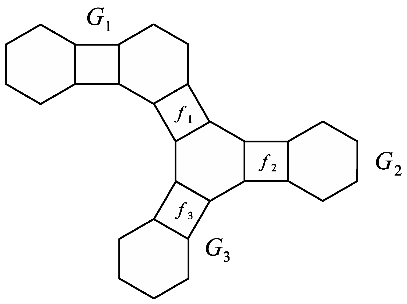
By adding edges $u_1{v}_3$, $v_1{u}_2$, and $v_2{u}_3$ to the disjoint union of graphs $G_1$, $G_2$, and $G_3$ satisfying Assumption 2, we obtain another generalized phenylene and denote it as $G_1\ast G_2\ast G_3$, see Figure 9 for an example. Moreover, let f be the hexagon of $G_1\ast G_2\ast G_3$ that contains edges $u_1{v}_3$, $v_1{u}_2$, and $v_2{u}_3$. It is easy to see that the graph $G_1\ast G_2\ast G_3$ also has a perfect matching. Similarly as in Section 3, for any $i\in \{1,2,3\}$ denote by $G_i^{\prime }$ the graph $G_i-u_i-v_i$ and by $G_i^{\prime \prime }$ the graph $G_i-f_i$.

In the next theorem, we calculate the MZZ polynomial of $G_1\ast G_2\ast G_3$.

Theorem 7.

If $G_1,G_2$, and $G_3$ are three generalized phenylenes satisfying Assumption 2, then the MZZ polynomial of $G=G_1\ast G_2\ast G_3$ can be computed as

$$\begin{array}{ccc}\hfill MZZ\left(G\right)& =& \prod _{j=1}^{3}MZZ\left(G_j\right)+(y+1)\prod _{j=1}^{3}MZZ\left(G_j^{\prime }\right)+zMZZ\left(G_1^{″}\right)MZZ\left(G_2^{\prime }\right)MZZ\left(G_3^{\prime }\right)\hfill \\ & +& zMZZ\left(G_1^{\prime }\right)MZZ\left(G_2^{″}\right)MZZ\left(G_3^{\prime }\right)+zMZZ\left(G_1^{\prime }\right)MZZ\left(G_2^{\prime }\right)MZZ\left(G_3^{″}\right).\hfill \end{array}$$

Proof. 

Suppose that we have the notation from Assumption 2 (see also Figure 9). By using Theorem 3 on the edge $u_1{v}_3$ of G one can obtain

$$\begin{array}{ccc}\hfill MZZ\left(G\right)& =& MZZ(G-u_1{v}_3)+MZZ(G-u_1-v_3)+yMZZ(G-f)\hfill \\ & +& zMZZ(G-f-f_1)+zMZZ(G-f-f_2)+zMZZ(G-f-f_3).\hfill \end{array}$$

It is easy to see that edges $v_1{u}_2$ and $v_2{u}_3$ do not belong to any perfect matching of $G-u_1{v}_3$ and, therefore, by Proposition 2 and Theorem 1 it follows

$$MZZ(G-u_1{v}_3)=MZZ(G-u_1{v}_3-v_1{u}_2-v_2{u}_3)=\prod _{j=1}^{3}MZZ\left(G_j\right).$$

In a similar way we can conclude that edges $v_1{u}_2$ and $v_2{u}_3$ belong to every perfect matching of $G-u_1-v_3$ (if this graph has a perfect matching) and, consequently, by Proposition 2 and Theorem 1 we obtain

$$MZZ(G-u_1-v_3)=MZZ(G-f)=\prod _{j=1}^{3}MZZ\left(G_j^{\prime }\right).$$

Furthermore, Theorem 1 implies

$$MZZ(G-f-f_1)=MZZ\left(G_1^{\prime \prime }\right)MZZ\left(G_2^{\prime }\right)MZZ\left(G_3^{\prime }\right)$$

and analogous formulas can be obtained for $MZZ(G-f-f_2)$ and $MZZ(G-f-f_3)$. By taking the obtained equalities into the first formula of this proof, we finally obtain the desired result. □

By using Theorem 7, we can reduce the problem of calculating the MZZ polynomial of any phenylene to the problem of calculating the MZZ polynomials of (reduced) phenylene chains and (reduced) modified phenylene chains, which can be easily solved by using Algorithms 1 and 2.

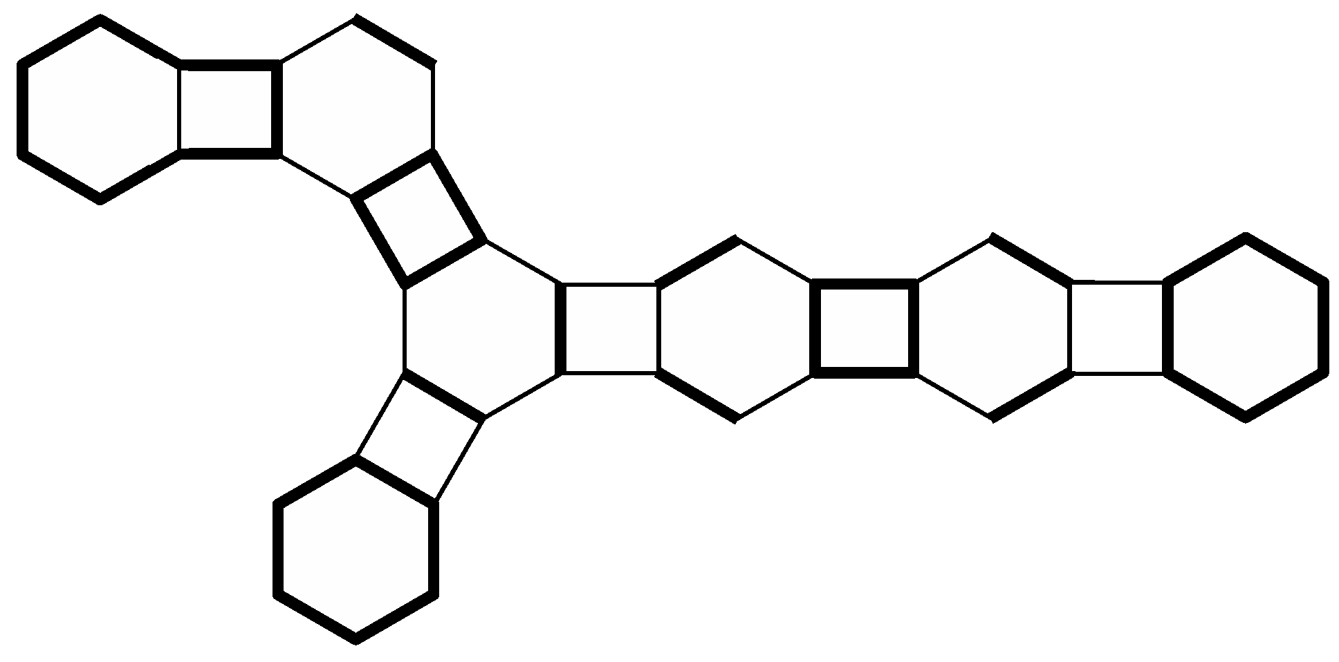
To show an example, let $G=G_1\ast G_2\ast G_3$ be a phenylene from Figure 10.

We can easily calculate that

$$\begin{array}{ccc}\hfill MZZ\left(G_1\right)& =& x^2+xy+y^2+xz+yz+5x+5y+5z+8,\hfill \\ \hfill MZZ\left(G_1^{\prime }\right)& =& y^2+x+4y+2z+5,\hfill \\ \hfill MZZ\left(G_1^{\prime \prime }\right)& =& x+y+z+3\hfill \end{array}$$

and

$$\begin{array}{ccc}\hfill MZZ\left(G_2\right)=MZZ\left(G_3\right)& =& x+y+z+3,\hfill \\ \hfill MZZ\left(G_2^{\prime }\right)=MZZ\left(G_3^{\prime }\right)& =& y+2,\hfill \\ \hfill MZZ\left(G_2^{\prime \prime }\right)=MZZ\left(G_3^{\prime \prime }\right)& =& 1.\hfill \end{array}$$

Therefore, Theorem 7 finally gives

$$\begin{array}{ccc}\hfill MZZ\left(G\right)& =& y^5+x^4+3x^{3}y+4x^2{y}^2+4x{y}^3+10y^4+3x^{3}z+7x^{2}yz+8x{y}^{2}z\hfill \\ & +& 8y^{3}z+3x^2{z}^2+5xy{z}^2+4y^2{z}^2+x{z}^3+y{z}^3+11x^3+27x^{2}y+32x{y}^2\hfill \\ & +& 44y^3+27x^{2}z+54xyz+56y^{2}z+21x{z}^2+29y{z}^2+5z^3+47x^2+93xy\hfill \\ & +& 108y^2+93xz+143yz+50z^2+97x+149y+133z+92.\hfill \end{array}$$

A more complicated case is obtained if we have a situation from Figure 11, where G is a phenylene containing two branched hexagons with one quadrilateral between them. To calculate $MZZ\left(G_1\right)$, we can firstly apply Corollary 2 for the face $f_1$. Note that in this case Theorem 7 and Corollary 2 both require to calculate $MZZ\left(G_1^{\prime \prime }\right)=MZZ(G_1-f_1)$. However, we notice that by Theorem 1 it holds $MZZ\left(G_1^{\prime \prime }\right)=MZZ\left(G_1^1\right)MZZ\left(G_1^2\right)$ since the edge $e^{\prime }$ can not belong to any perfect matching of $G_1^{\prime \prime }=G_1-f_1$. Here $G_1^1$ and $G_1^2$ are the two connected components of the graph $G_1^{\prime \prime }-e^{\prime }$ (see Figure 11).

6. Conclusions

In the paper, we have introduced the MZZ polynomial for any generalized phenylene. By definition, this polynomial counts the number of so called (4,6,8)-Clar covers with specific numbers of 4-cycles, 6-cycles, and 8-cycles. We provided several results that enable us to calculate the MZZ polynomial of a generalized phenylene by using the MZZ polynomials of subgraphs of the original graph. Then, we focused on phenylene chains and developed an efficient algorithm that calculates the MZZ polynomial for any (reduced) phenylene chain in linear time with respect to the number of hexagons (assuming that addition and multiplication of polynomials of three variables can be calculated in constant time). Furthermore, the main result of Section 5 can be used to calculate the MZZ polynomial of a phenylene with branched hexagons.

Regarding the future work, it would be interesting to investigate the chemical applicability of the MZZ polynomial. In particular, relations between the MZZ polynomial and some energy-based quantities of phenylenes can be tested. Moreover, it would be nice to obtain new mathematical properties of the MZZ polynomial and investigate this polynomial for some special classes of phenylenes.

References

- Cyvin, S.J.; Gutman, I. Kekulé Structures in Benzenoid Hydrocarbons; Springer: Berlin, Germany, 1988. [Google Scholar]
- Gutman, I.; Cyvin, S.J. Introduction to the Theory of Benzenoid Hydrocarbons; Springer: Berlin, Germany, 1989. [Google Scholar]
- Gojak, S.; Gutman, I.; Radenković, S.; Vodopivec, A. Relating resonance energy with Zhang-Zhang polynomial. J. Serb. Chem. Soc. 2007, 72, 673–679. [Google Scholar] [CrossRef]
- Clar, E. The Aromatic Sextet; John Wiley & Sons: London, UK, 1972. [Google Scholar]
- Zhang, H.; Zhang, F. The Clar covering polynomial of hexagonal systems I. Discrete Appl. Math. 1996, 69, 147–167. [Google Scholar] [CrossRef]
- Fowler, P.W.; Myrvold, W.; Vandenberg, R.L.; Hartung, E.J.; Graver, J.E. Clar and Fries structures for fullerenes. Art Discret. Appl. Math. 2022. [Google Scholar] [CrossRef]
- Graver, J.E.; Hartung, E.J.; Souid, A.Y. Clar and Fries numbers for benzenoids. J. Math. Chem. 2013, 51, 1981–1989. [Google Scholar] [CrossRef]
- Klavžar, S.; Salem, K.; Taranenko, A. Maximum cardinality resonant sets and maximal alternating sets of hexagonal systems. Comput. Math. Appl. 2010, 59, 506–513. [Google Scholar] [CrossRef]
- Zhai, S.; Alrowaili, D.; Ye, D. Clar structures vs Fries structures in hexagonal systems. Appl. Math. Comput. 2018, 329, 384–394. [Google Scholar] [CrossRef]
- Langner, J.; Witek, H.A. Interface theory of benzenoids. MATCH Commun. Math. Comput. Chem. 2020, 84, 143–176. [Google Scholar]
- Li, G.; Pei, Y.; Wang, Y. Clar Covering polynomials with only real zeros. MATCH Commun. Math. Comput. Chem. 2020, 84, 217–228. [Google Scholar]
- Tratnik, N.; Ye, D. Resonance graphs on perfect matchings of graphs on surfaces. Graphs Comb. 2023, 39, 68. [Google Scholar] [CrossRef]
- Zhang, H. Z-transformation graphs of perfect matchings of plane bipartite graphs: A survey. MATCH Commun. Math. Comput. Chem. 2006, 56, 457–476. [Google Scholar] [CrossRef]
- Zhang, H.; Shiu, W.C.; Sun, P.K. A relation between Clar covering polynomial and cube polynomial. MATCH Commun. Math. Comput. Chem. 2013, 70, 477–492. [Google Scholar]
- Che, Z. Peripheral convex expansions of resonance graphs. Order 2021, 38, 365–376. [Google Scholar] [CrossRef]
- Žigert Pleteršek, P. Equivalence of the generalized Zhang-Zhang polynomial and the generalized cube polynomial. MATCH Commun. Math. Comput. Chem. 2018, 80, 215–226. [Google Scholar]
- Furtula, B.; Radenković, S.; Redžepović, I.; Tratnik, N.; Žigert Pleteršek, P. The generalized Zhang-Zhang polynomial of benzenoid systems—Theory and applications. Appl. Math. Comput. 2022, 418, 126822. [Google Scholar] [CrossRef]
- Radenković, S.; Redžepović, I.; Furtula, B.; Đorđević, S.; Tratnik, N.; Žigert Pleteršek, P. Relating vibrational energy with Kekulé- and Clar-structure-based parameters. Int. J. Quantum Chem. 2022, 122, e26867. [Google Scholar] [CrossRef]
- Gutman, I. Algebraic structure count of linear phenylenes. Indian J. Chem. 1993, 32A, 281–284. [Google Scholar]
- Gutman, I. Algebraic structure count of linear phenylenes and their congeners. J. Serb. Chem. Soc. 2003, 68, 391–399. [Google Scholar] [CrossRef]
- Gutman, I.; Furtula, B. A Kekulé structure basis for phenylenes. J. Mol. Struct. Theochem. 2006, 770, 67–71. [Google Scholar] [CrossRef]
- Brinkmann, G.; Caporossi, G.; Hansen, P. A constructive enumeration of fusenes and benzenoids. J. Algorithms 2002, 45, 155–166. [Google Scholar] [CrossRef]
Figure 1.
A benzenoid graph B and the corresponding phenylene G.
Figure 2.
A (4,6,8)-Clar cover of a phenylene.
Figure 3.
Generalized phenylene G in Theorem 3.
Figure 4.
Graph in Theorem 5.
Figure 5.
(a) The basic compound of a phenylene P and (b) the graph .
Figure 6.
Linear phenylene chain .
Figure 7.
A phenylene chain and the corresponding reduced phenylene chain .
Figure 8.
A modified phenylene chain and the corresponding reduced modified phenylene chain .
Figure 9.
A generalized phenylene .
Figure 10.
A phenylene .
Figure 11.
A phenylene , where and are connected components of .
Disclaimer/Publisher’s Note: The statements, opinions and data contained in all publications are solely those of the individual author(s) and contributor(s) and not of MDPI and/or the editor(s). MDPI and/or the editor(s) disclaim responsibility for any injury to people or property resulting from any ideas, methods, instructions or products referred to in the content. |
© 2023 by the author. Licensee MDPI, Basel, Switzerland. This article is an open access article distributed under the terms and conditions of the Creative Commons Attribution (CC BY) license (https://creativecommons.org/licenses/by/4.0/).
Share and Cite
MDPI and ACS Style
Tratnik, N. The Multivariable Zhang–Zhang Polynomial of Phenylenes. Axioms 2023, 12, 1053. https://doi.org/10.3390/axioms12111053
AMA Style
Tratnik N. The Multivariable Zhang–Zhang Polynomial of Phenylenes. Axioms. 2023; 12(11):1053. https://doi.org/10.3390/axioms12111053
Chicago/Turabian StyleTratnik, Niko. 2023. "The Multivariable Zhang–Zhang Polynomial of Phenylenes" Axioms 12, no. 11: 1053. https://doi.org/10.3390/axioms12111053
Note that from the first issue of 2016, this journal uses article numbers instead of page numbers. See further details here.