1. Introduction
Graph theory is like a special tool in mathematics that helps us to understand how things are connected. Graph theory started with K
nigburg’s seven bridge problem [
1]. It is like a universal language for studying relationships between various things, like friendships or the structure of molecules. It is kind of like drawing a map with dots and lines to represent complicated systems. This helps us solve problems, make models of real-life situations, and figure out how things are connected. Spectral graph theory [
2] introduces a special kind of wonder to graph theory. It takes us into the fascinating world of eigenvalues and eigenvectors, where graphs share their mysteries through mathematical beauty. The spectrum of a graph unveils its hidden patterns, helping us organize information, explore connections, and understand how networks work. Spectral graph theory plays a crucial role in the development of Graph Neural Networks (GNNs), a subfield of deep learning. GNNs have gained prominence in recent years for their ability to process data structured as graphs, making them applicable to a wide range of domains, from social network analysis to recommendation systems. Spectral graph theory provides the mathematical foundation for understanding the propagation of information through graphs, which is essential in GNNs [
3]. While spectral methods are powerful, they can be computationally intensive, especially for large graphs. Implementing these techniques in AI (artificial intelligence) and ML (machine learning) applications might require significant computational resources.
Throughout the article, we consider simple connected graphs. Let
be a simple connected graph with vertex set
and edge set
, respectively. The adjacency matrix of a graph
of order
n is an
square symmetric matrix
, whose
th entry is the number of edges between the vertices
i and
j. If two vertices are adjacent in a graph
, they are called neighbors, so the neighborhood of a vertex
in a graph
is denoted as
and is defined as
The cardinality
is called the degree of vertex
and is denoted as
. If
, then
is called an isolated vertex, and if the degree of a vertex
is 1 i.e.,
, then that vertex is called a terminal vertex or pendant vertex. A vertex is called quasipendant if it is adjacent to a pendant vertex (for notations, see reference [
4]).
A weighted graph is one in which the edges are assigned weights. Weighted graphs model road networks, flight connections, and shipping routes. They help optimize routes, minimize costs, and manage the flow of goods and people efficiently. The shortest path problem is one of the best real-life examples of weighted graphs. In social media and sociology, weighted graphs represent relationships with varying strengths. They enable the identification of influential individuals, community detection, and targeted advertising. Weighted graphs assist in personalized recommendations on platforms like Amazon and Netflix. They enhance user experience by suggesting products or content based on preferences and connections. In finance, these graphs model correlations between financial instruments, helping with risk assessment, portfolio optimization, and market analysis. Weighted graphs are used to represent protein interaction networks, metabolic pathways, and genetic relationships. They aid in understanding complex biological systems and drug discovery. Electrical power systems use weighted graphs to model energy distribution and grid stability. They ensure efficient power flow and prevent blackouts.
Let
be a simple connected graph. Let
denote the weighted graph obtained from
after applying the weight function
on the edge set of
, where
is the set of all positive weight functions defined on the edge set of
. The adjacency matrix of a graph
of order
n is defined as
A graph
is said to be non-singular if det
and singular otherwise. The eigenvalues of a graph
are the roots of the characteristic polynomial of its adjacency matrix
; since
is symmetric, all of its roots, or eigenvalues, are real. The set consisting of all the eigenvalues
of a graph
is called its spectrum.
where
is the multiplicity of each
. The spectral radius of a finite graph is determined by taking the largest absolute value within its graph spectrum. Spectral graph theory explores the connection between a graph’s structural features and its eigenvalues. This is highly relevant in various domains such as social network analysis, transportation systems, communication networks, and even biological networks like protein–protein interaction networks. The insights gained from spectral graph theory can lead to more efficient network designs, improved routing algorithms, and better decision-making in network-related applications. Spectral clustering techniques based on spectral graph theory are used for data partitioning and clustering. Spectral graph theory is also used for signal processing on graphs. Community detection in complex networks, such as identifying groups of individuals with shared interests in a social network, relies on spectral graph theory. The eigenvalues of a graph provide insights into the graph’s topological attributes, including its size, order, the count of triangles, the total number of closed walks of different lengths, whether the graph is bipartite, and its regularity [
2]. For example,
A graph is bipartite if and only if its spectrum is symmetric around zero, that is, for each
there exists
[
2].
If , then is a complete multipartite graph.
If , then is a complete graph.
Several graph theoretic properties have been discussed in references [
5,
6,
7,
8,
9,
10,
11]. In reference [
12], the authors presented techniques from graph theory to assess the ranking of substations within an electric power grid. It specifically applies spectral graph theory and outlines various ranking algorithms. A novel mining algorithm rooted in spectral graph theory was introduced in reference [
13]. The algorithm initially constructed an alarm association model using time series data. It then treated the alarms database as a high-dimensional structure, considering alarms with shared characteristics as integral components of this structure. Leveraging spectral graph theory, the algorithm uncovered the underlying mapping of a low-dimensional structure embedded within a high-dimensional space. The experimental results, based on both synthetic and real datasets, demonstrated that this approach not only uncovered associations among alarms but also identified faults in the telecommunications network through spectral graph transformations. Furthermore, an innovative approach to create wavelet transforms for functions defined on the nodes of any finite weighted graph was introduced in reference [
14]. This approach was based on defining scaling using the graph’s analogue of the Fourier domain, namely the spectral decomposition of the discrete Laplacian graph.
In reference [
15], the authors established the concept of a reciprocal eigenvalue property (property
) for the nonsingular graphs. A nonsingular graph
holds property
if the reciprocal of each eigenvalue is also an eigenvalue of
; in addition, if the multiplicity constraint is applied on the eigenvalues and their reciprocals, then that graph
holds a strong reciprocal eigenvalue property (property
).
The anti-reciprocal eigenvalue property (property
) of graphs was introduced by Lagrange in reference [
16]. A nonsingular graph
holds property
if the negative reciprocal of each eigenvalue is also an eigenvalue of
; in addition, if the multiplicity constraint is applied on the eigenvalues and their negative reciprocals, then that graph
holds a strong anti-reciprocal eigenvalue property (property
).
Nonsingular trees with property
were studied in 1978 under the titles,
symmetric property [
17] and
property C [
18]. Barik et al. renamed this property as “property
” in 2006, and they also introduced property
. They demonstrated that these two features are identical for nonsingular trees [
19]. Moreover, in reference [
20], it is proved that properties
and
are also equivalent for weighted trees and they continued studying the nonsingular trees in two ways. Firstly, they studied the characterization of the set of all graphs whose inverses are nonsingular trees. Secondly, they investigated the extent of property
for weighted trees and characterized the property for all trees with eight vertices or more, under specific conditions on the weights. The authors provided a subclass of connected bipartite graphs with unique perfect matching, proving that it satisfies properties
and
if appropriate limitations on the weight function are enforced [
21]. However, the general equivalence of these two properties for any nonsingular graph has not been established. In reference [
22], the authors established that these properties are not equivalent in general. In reference [
23], the structure of a unicyclic graph with property
was examined. This study revealed that “such a graph is typically bipartite and took on a corona structure, except when it had a girth of four”. In the exceptional case where it is not a corona, the paper demonstrated that the graph could assume one of three distinct structures. The paper also presented families of unicyclic graphs with property
, each corresponding to one of these specific structures.
For a connected bipartite graph
with a unique perfect matching
M, the weighted graph
satisfies property
for all
if and only if
is a corona, according to Bapat et al. [
24].
J. D. Lagrange [
16] studied property
for the zero-divisor graphs of finite commutative rings with non-zero divisors for the first time in 2012. Hameed et al. [
25] investigated a family of graphs with unique perfect matching and diagonal entries of zero in the inverse of their adjacency matrix. The authors showed that this family does not satisfy property
, not even for a single weight function
w.
Ahmad et al. [
26] explored the property
for the class of connected simple weighted graphs with unique perfect matching
M, denoted by
, in 2020. They demonstrated that,
is a corona if and only if, the weighted graph
satisfies the property
for any
. They also investigated the property
for several non-corona graph families [
27], and Barik et al. [
28] extended these families. They created the noncorona graph classes by linking each vertex of a finite number of copies of corona cycles of varying finite length to nondependent vertices of
in such a manner that no corona cycle is linked to more than one quasipendant vertex. These families were later generalized for weighted graphs in [
29]. In reference [
30], the authors investigated some families of graphs with property
but not
. Later on, signed graphs with property
were investigated in reference [
31]. In reference [
32], the authors introduced a new family of graphs named flabellum graphs and, with the help of this family, they constructed several families of graphs with property
.
In [
33], Barik et al. constructed some classes of unweighted nonbipartite graphs using complete graph
and a copy of the path graph
. These families of graphs satisfy property
but not
for simple weights 0 and 1. In this article, an investigation is carried out to answer the following question: “what happens if we assign weight functions on edge sets of these classes?” It is interesting to note that, under certain weights, these families of graphs satisfy property
; however, if some of these weights are changed with specific conditions, the same families of graphs satisfy property
but not
.
3. Main Results
In a previous work by Barik et al. [
33], specific classes of unweighted nonbipartite graphs were created using a complete graph and a copy of the path graph. They investigated how these families of graphs satisfy the property
but not
. In this section, we aim to determine the weight functions that enable these nonbipartite graph classes to satisfy property
or property
. Consider the complete graph
and one copy of
with vertex set
.
Definition 4 (ref. [
33])
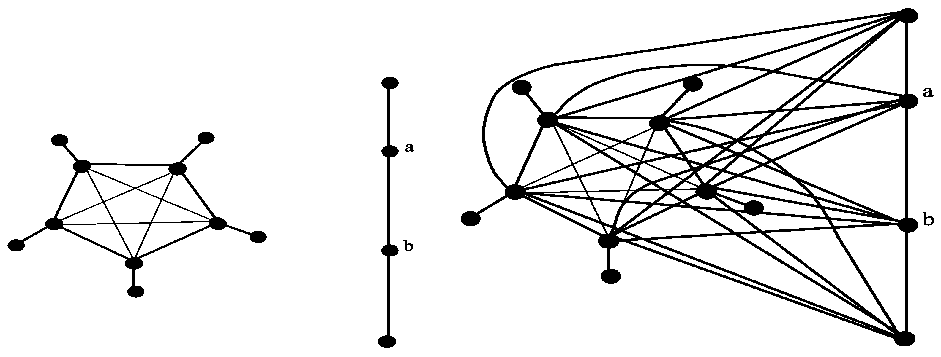
. Let , be the graph obtained using the corona and in such a way that each non pendant vertex of is joined with each vertex of by an edge; the order of this graph is . For example,
can be obtained from
and
, as shown in
Figure 1. In reference [
33], the authors proved that this graph is very close to satisfy property
. We investigated how, if we assign weights to some of the edges of the graph under specific conditions, then this graph will satisfy property
.
The adjacency matrix of the path graph or can be written as follows:
,
then, where and .
Let
, then
where
Following the same logic as in (4), we can see that
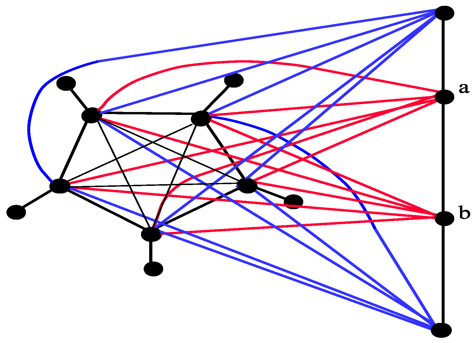
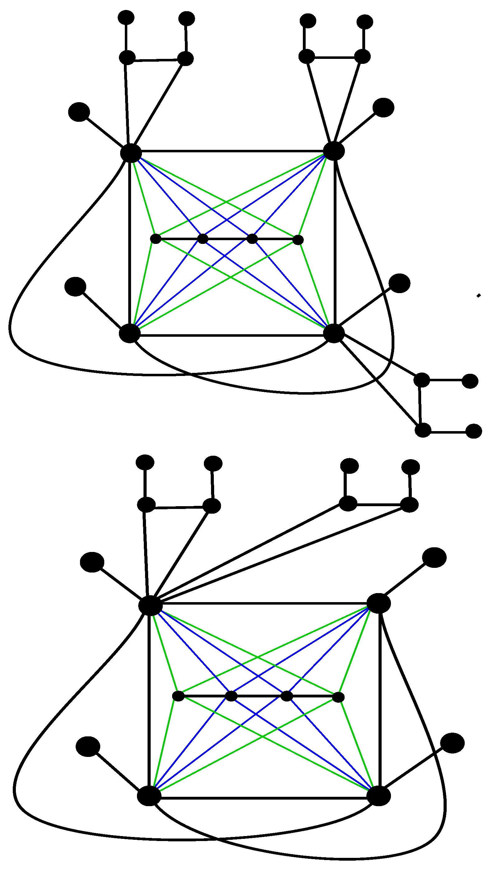
Definition 5. Let be a weighted graph obtained from (defined in Definition 4) by assigning a weight function to the edge set of defined as,For example, , as shown in Figure 2, has the following weight function Theorem 1. The graph , as defined in Definition 5, satisfies property .
Proof. The adjacency matrix of the graph
can be written as,
Thus,
Since the polynomials
and
satisfy property
from Lemma 1, thus
satisfies property
. □
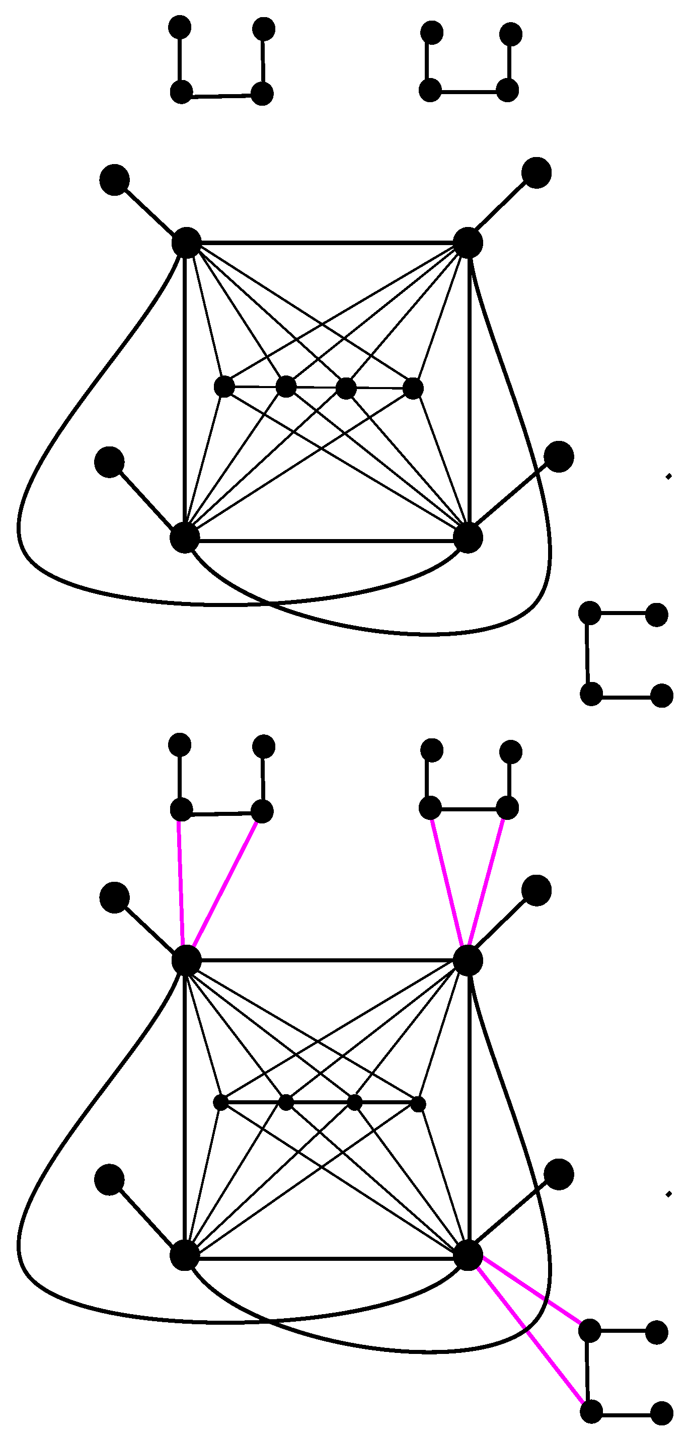
Remark 1. Let . The weighted graph in Definition 5 can be further generalized by assigning the following weight function:It can be shown that satisfies property using a similar argument as in Theorem 1. Definition 6. Consider the graph , as defined above. Let , be k quasipendant vertices in . Let be the graph obtained from (defined in Definition 4), by attaching a copy of at each quasipendant vertex , of in such a way that each nonpendant vertex of is attached to by an edge. Assign the weight function on the edge set of defined asThus, the order of the graph is . For example, as shown in Figure 3, which is obtained from and three copies of , where Theorem 2. The graph , as defined in Definition 6, satisfies property but not for .
Proof. The adjacency matrix of
can be written as
Let
,
and
where
and
Thus, the adjacency matrix of
can be written as
Then,
from Lemma 3 and Observation 1, we have
Since is palindromic and the power of is greater than the power of . Thus, for , satisfies property but not . □
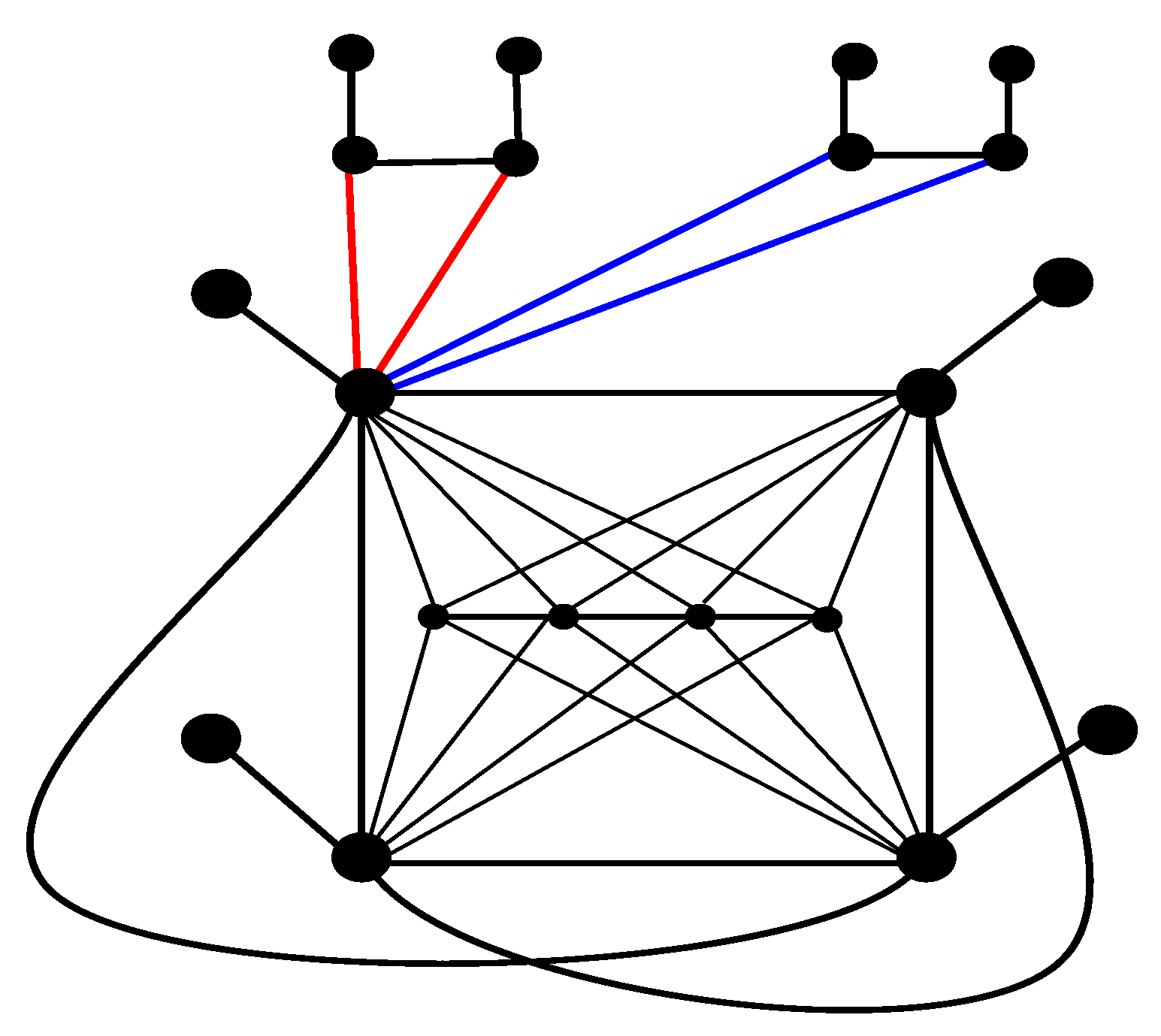
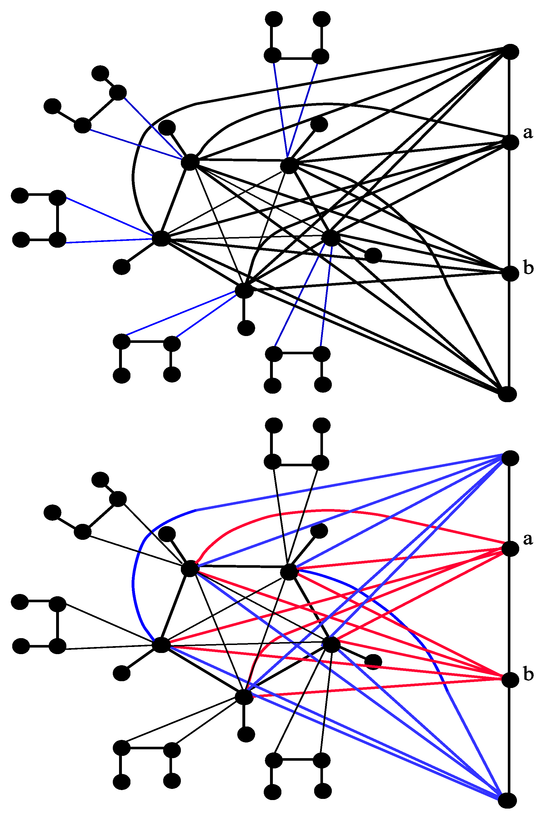
Remark 2. If the k copies of in Definition 6 are named as , for . The weighted graph can be further generalized by assigning the following weight function:Then, it can be shown that satisfies property but not using a similar argument as in Theorem 2. Definition 7. Consider the graph defined in Definition 4. Take copies of , namely and attach nonpendant vertices of all these copies to one quasipendant vertex of . Now, a weighted graph can be obtained from this graph by assigning a weight function to the edge set as follows:For example, , which is obtained from one copy of and copies of , namely and , as shown in Figure 4, where the weights are assigned to the red and blue edges, respectively, according to the following weight function. Theorem 3. The graph , as defined in Definition 7, satisfies property but not .
Proof. The adjacency matrix of
can be written as
where
Thus,
where
, then
Using observation (4) and (5)
where
is a palindromic polynomial which satisfies property . Moreover, the multiplicities of roots differ due to the polynomials and . We can see that satisfies property but not . □
Now, the following question arises: ‘is it possible to assign weights to some edges so that the classes defined in Definitions 6 and 7 satisfy property ?’ To answer this question, we assign weights to some particular edges and, consequently, the families of nonbipartite weighted graphs with property are given in Definitions 8 and 9. We recall that the graph is obtained using the coronas and in such a way that each non-pendant vertex of is joined with each vertex of by an edge.
Definition 8. Consider the graph , as defined in Definition 6. A new weighted graph can be obtained if we replace the weight function by , defined aswhere and are the graphs used in the construction of . For example, , as shown in Figure 5, where Definition 9. We now introduce the graph obtained from by changing weight function to , defined aswhere and are the graphs used in the construction of . For example, , as shown in Figure 5, with weight function Theorem 4. The graph , defined in Definition 8, satisfies property .
Proof. Recall that,
Let
,
and
, where
and
Thus, the adjacency matrix of
can be written as,
Then, the characteristic polynomial of
is
using observations (4) and (5)
where
satisfies property
from Lemma 1. Thus, the graph
satisfies property
. □
Theorem 5. The graph , as defined in Definition 9, satisfies property for .
Proof. Remember that, and
Let , and where, for
Thus, .
Then, using direct calculations, the characteristic polynomial of
can be written as
using observations (4) and (5)
.
We see that satisfies property from Lemma 1. □
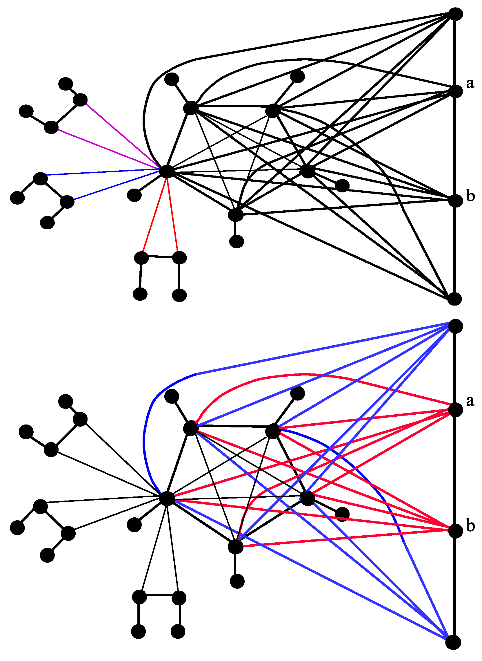
Example 1. Consider the graph , as shown in Figure 2. The weight function defined on the edge set of isThe red edges are assigned weight , the blue edges are assigned weight 11, and all the remaining edges are assigned weight 1. The spectrum of is shown in Table 1. We can easily see that this graph satisfies property . Example 2. Consider the graph . It is obtained from copy of and copies of according to Definition 6. The following weight function is applied on the graph :All the blue edges are assigned weight 7, as shown in Figure 6. The spectrum of is shown in Table 2. We can easily see that satisfies property but not . In the graph , if we change the weight function to (according to the Definition 8), thenThe graph with a weight function is shown in Figure 6. In Table 3, the spectrum of the weighted graph is given. Example 3. Consider the graph , as shown in Figure 7. This graph is obtained from copy of and copies of (namely and ) according to Definition 7. The weight function applied to the graph is as follows:Here, the weights , , and are assigned to the purple, blue, and red edges, respectively. The spectrum of is given in Table 4. We can easily see that satisfies property . In the graph , if we change weight function to according to Definition 9, then the resulting graph is named , as shown in Figure 7. The weight function of follows:Table 5 shows the spectrum of ; it can be seen that it satisfies property . 


