
Eigenvalue −1 of the Vertex Quadrangulation of a 4-Regular Graph


Department of Mathematics, Ariel University, Ariel 4070000, Israel
Axioms 2024, 13(1), 72; https://doi.org/10.3390/axioms13010072
Submission received: 24 December 2023
/
Revised: 15 January 2024
/
Accepted: 16 January 2024
/
Published: 22 January 2024
(This article belongs to the Special Issue Spectral Graph Theory, Molecular Graph Theory and Their Applications)
Abstract
:The vertex quadrangulation of a 4-regular graph G visually looks like a graph whose vertices are depicted as empty squares, and the connecting edges are attached to the corners of the squares. In a previous work [JOMC 59, 1551–1569 (2021)], the question was posed: does the spectrum of an arbitrary unweighted graph include the full spectrum of the tetrahedron graph (complete graph )? Previously, many bipartite and nonbipartite graphs with such a subspectrum have been found; for example, a nonbipartite variant of the graph . Here, we present one of the variants of the nonbipartite vertex quadrangulation of the octahedron graph O, which has eigenvalue of multiplicity 2 in the spectrum, while the spectrum of the bipartite variant contains eigenvalue of multiplicity 3. Thus, in the case of nonbipartite graphs, the answer to the question posed depends on the particular graph . Here, we continue to explore the spectrum of graphs . Some possible connections of the mathematical theme to chemistry are also noted.
Keywords:
vertex quadrangulation; truncation; characteristic polynomial; graph spectrum; (matrix, graph) divisor; equitable partition; straight-ahead walk; polychromatic coloring; band decomposition; ribbon graphMSC:
15A18; 05C50; 05C151. Introduction
Spectral graph theory is increasingly used in chemistry to study molecular graphs [1,2,3,4,5,6,7,8,9,10,11,12,13,14]. Since molecular graphs are used to solve various specific problems, studying their eigenvalue spectra can help solve these problems [12]. Without being able to consider this topic in detail, we can name only a few examples of it. But some aspects that are not mentioned here and are necessary for further presentation will be considered directly in the main text. The most common use of eigenvalues (of the adjacency matrix) of molecular graphs is for calculating electronic energy levels in the Hückel molecular orbital method [1,2,3,4,5,6,7,8,9,10,11,12,13,14]. The least modulus positive and negative eigenvalues determine the energy gap, which determines whether a substance will be a conductor, a semiconductor, or an insulator for electric current [14]. The spectrum of the molecular graph in the Hückel method also determines the electronic energy of the molecule and thereby determines its stability [11].
In chemistry, there are problems that consider substitutional isomers when there is constrained positioning of ligands on a molecular skeleton [15,16,17,18]. One constraint involves ‘restrictive ligands’ where two ligands (substituting radicals) of the same or different types are forbidden to occupy adjacent sites in a molecular skeleton. This can arise because of steric hindrance, or because of functional groups that, in close proximity in the molecule, react to eliminate an “undesirable neighbor”. For instance, no pair of –OH groups attach to the same C atom in a molecular skeleton [15]. In another case, malonic acid residues decarboxylate, leaving no more than one decarboxylation in each residue. Such chemistry problems make it possible to model a molecule with substituents in the form of a molecular graph, in which substituents of different types are distinguished by different coloring of the corresponding vertices of the graph. Then, in a number of cases, spectral graph theory comes to the rescue.
Here, we can adapt the following example from the literature for our discussion [19]. A perfect star packing in a cubic (3-regular) graph G is a spanning subgraph (covering all vertices) of G whose every component is isomorphic to the 4-vertex star graph (with a central vertex and three incident edges). The authors investigated which fullerene graphs allow such packings. It turned out that all fullerene graphs that admit such a packing must have at least one eigenvalue as a necessary (but not sufficient) condition; otherwise, it is impossible. If we focus only on all the central vertices, we will notice that all these vertices of the fullerene graph are located at a distance of no closer than three edges from one another. That is, with at least two intermediate vertices on the shortest path connecting any pair of central vertices of the stars. In total, if the graph is completely covered by maximal stars, there will be exactly central vertices, where n is the number of vertices in the graph or the number of carbon atoms in the corresponding fullerene molecule. As a result, we are talking about the potential possibility of attaching to such a molecule of bulky substituents with the condition that they will not be located closer than what we have defined for this on the graph.
However, we must admit that the use of spectral theory is not the only way to solve problems similar to the one we considered above. Let denote the square of a graph G in which two vertices are adjacent if and only if they are at a distance of ≤2 in the graph G. (Thus, the graph is obtained from the graph G by adding new edges connecting all pairs of vertices that are at a distance of 2 in G.) Then, the last nonzero coefficient of the independence polynomial of [20], which is called the independence number of, in the case of interest to us is equal to , which coincides with the number mentioned in the first example, where the eigenvalue of the molecular graph plays a special role. Of course, speaking about the role of this eigenvalue, we are not disputing the role of any other values, but we will be mainly interested in the eigenvalue . In addition, we note that there are other “not our” studied cases [21,22,23,24,25,26,27], when this eigenvalue provides some structural information about the molecules whose graphs have it.
There are several possible topics that, in a broader context, could lead to the type of graphs indicated in the title of this text. One such topic, already sufficiently described in our previous work [24], is the spectra of graphs with decorated vertices. In our particular case, this means quadrangulating the vertices of the original 4-regular graph, or, in a simple loose definition, replacing each of its vertices, depicted as a point, with a quadrilateral and attaching connecting edges to the corners of adjacent quadrilaterals.
When dealing with operations on graphs, a graph spectra specialist usually seeks to find a formula that uniquely determines the eigenvalues of the resulting graph in terms of the eigenvalues of the original graph G and the auxiliary graph, if any (in our case, this is the 4-vertex cycle ). Unfortunately, the vertex quadrangulation cannot have such a general formula, since, in the general case, there are many nonisomorphic quadrangulations of the same graph G that can have different spectra. Therefore, our attention is mainly focused on studying a strictly defined type of quadrangulation, for which it is possible, if not to describe the entire spectrum, then at least to prove the inclusion in it of the full spectrum of the complete graph (being a skeletal graph of a tetrahedron): . In the case of bipartite vertex-quadrangulated graphs, this becomes the inclusion of the full spectrum of the skeletal graph of the cube——where each superscript means the multiplicity of the corresponding eigenvalue. Moreover, of particular interest is the subcase when there is not just inclusion of the spectrum of , but also a divisor isomorphic to this graph (which in the general case is not always realized) [24].
Another approach to our work can be through the consideration of special proper colorings of the resulting quadrangulated graphs . Here, a problem can be formulated that, as it turns out, is equivalent to a spectral one. We are interested in the case when graph ’s vertices are colored in four different colors, with an equal number of vertices of each color. This prevents any pair of vertices of the same color from being at a distance less than 3 from each other (as in the first case discussed above). A situation in chemistry that illustrates what has been said is placing four types of substituents in a molecule (using the same numbers of each of them), when, due to their size or interactions, they cannot be placed in adjacent sites in a molecule or next to in distance (the case is quite familiar in chemistry). More generally, other types of colorings are also important.
Speaking of chemical applications, we can recall the synthetic aspects of chemistry, where graphs, and therefore any useful information about them, can play a role. One such example has been discussed previously in [24], the desired synthesis of a two-dimensional polymer of cyclobutadiene, , which has not yet been realized. If it comes true, then in the future it will also become possible to synthesize the same polymer directly using cheaper and more readily available acetylene , from which cyclobutadiene is obtained. Really existing polymers of a different chemical nature are already known, which can be represented by the graph .
To the above aspects, we can add aspects related to the embeddings of the graphs under consideration on surfaces and a certain type of walks on these graphs. We will try to use all relevant nonspectral branches of graph theory to solve our spectral problems.
Here, we move on to the next mathematical sections with a more rigorous formulation of the problems we solve and some theorematic results concerning the spectra of vertex-quadrangulated graphs , and especially their eigenvalue .
2. Preliminaries
Let be a simple connected graph with the vertex set V and the edge set E; . A spanning subgraph H of G contains all vertices of G . An r-factor of a graph G is an r-regular spanning subgraph (all of whose vertices have valency r). A 1-factor is called a perfect matching; it is a cover of G by pairwise nonincident edges. A 2-factor is an arbitrary vertex cover of G by cycles. Next, take a cycle (quadrangle) and denote one pair of its diagonal vertices by numbers 1 and 2, respectively. A garland [24] in our text is a cyclic construct formed from p cycles (quadrangles), where vertex 1 of each copy of is connected by an edge to vertex 2 of an adjacent copy of , and conversely. Thus, each quadrangle in has two diagonal vertices of valency 3 and two other diagonal vertices that retain valency 2 and are not used in the construction for contacts.
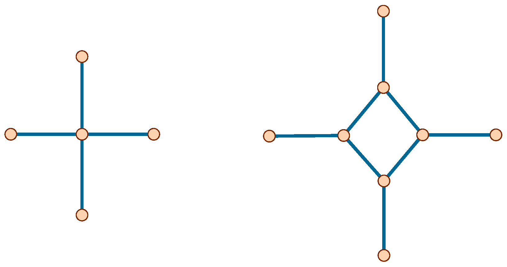
A vertex u of the 4-regular graph G is incident to the edges (following their cyclic order in G embedded in a surface). One can replace the vertex u with a square and connect by an edge each vertex of the square to vertex of G (see Figure 1). The application of such an operation to every vertex of G produces the vertex quadrangulation of G; see Figure 3, upper left. The vertex quadrangulation of a 4-regular graph G visually looks like a graph whose vertices are depicted as empty squares, and the connecting edges are attached to the corners of the squares. The quadrangulation graph is a 3-regular (cubic) graph.
The contraction to points of all quadrangles in always returns the original graph G. In the general case, one can obtain a set of nonisomorphic vertex quadrangulations of the same original graph G (see Figure 2). Later, we will specify exactly what type of quadrangulation we will need for our reasoning.
As an example, we note that the skeleton graph of the truncation [28,29] of any polyhedron with a 4-regular skeleton graph P is also a vertex quadrangulation of P; see [24] and Figure 2, left. Other examples are a rhombitruncated cuboctahedron and a rhombitruncated icosidodecahedron.
The characteristic polynomial of an arbitrary graph Γ is defined as the characteristic polynomial of its adjacency matrix [30]:
where I is the identity matrix of consistent dimensions. Also, the spectrum of a graph Γ is the set of all eigenvalues of its adjacency matrix A, or all roots of the characteristic polynomial [30].
It is briefly mentioned that the eigenvalues of the molecular graph in the simple Hückel method in chemistry are associated with electron energy levels in the molecule (see Ch. 8 in [1,2,3,4,5,6,7,8,9,10,11,12,13,14,30]). So, in the case of a molecule consisting of identical atoms, , where are the energy of the i-th Hückel orbital, the Coulomb integral of the atom, and the resonance integral, respectively, .
The theme of the use of the spectral theory of graphs now often arises in chemistry. This was also the case in our previous work [24], and here we further continue it. Examination of the graph spectrum of a putative molecular graph may provide some assistance in the mathematical planning of the synthesis of new molecules or logically reject the initial candidate choice.
Here, it is necessary to explain our current interest in graphs . To do this, we use an example from [24], in which serves as a template for an envisioned molecule.
The graph can be represented as the union of two edge-disjoint spanning subgraphs and , where is a 2-factor whose components are vertex-disjoint quadrangles, and is a 1-factor whose components are the remaining (connecting) edges of . The chemical representation of the quadrangles in the subgraph is the four-atomic cycles (rings) in the corresponding molecule. In the envisioned polycyclobutadiene molecule represented by [24], each such ring is formed by four carbon atoms and belongs to the cyclobutadiene monomeric unit, , of this polymer. Here, we recall that chemistry has taken the approach to depicting (organic) molecules with hydrogen-depleted graphs (ignoring the hydrogen atoms in the molecule), which can also represent a multiple chemical bond with a single edge. Thus, the representation of a cyclobutadiene molecule with two nonincident double bonds in its ring by such a graph gives us a simple 4-vertex cycle , which also represents a single monomeric unit in a polymer. The concomitant subgraph is a perfect matching of , which in chemistry corresponds to the Kekulé structure of the corresponding molecule. The subgraph in our context does not describe any initial substance, but represents exactly those chemical bonds between cyclobutadiene rings that should appear in the target polymer molecule [24]. Note that the same envisioned molecule is also the polymer of acetylene , which can be used to synthesize it.
Also in chemistry, it is often customary to consider whole radicals (chemically bonded groups of atoms) as separate generalized atoms. Regardless of the nature of such groups, they can be denoted by one letter when writing structural formulas. Such formulas allow one to further represent them graphically in a simplified form of molecular graphs, where a grouping of atoms designated by one letter corresponds to one vertex of the molecular graph. Due to that, one has more opportunities to look for examples of molecules that can be represented by vertex-quadrangulated graphs. A class of such real molecules is the organotin polymers with the general formula [31] or shorter , where is a methyl, ethyl, n-butyl, or phenyl radical, and G represents the group. The entire connected molecular network of (including all quadrangles and links between them) is formed by bonds, which can also be conceptualized as bonds, where the entire group G behaves like a generalized atom. Each Sn (res. O) atom in the network is bonded to three O (res. Sn) atoms, and the attached radicals R are projected outside the network [31].
An important notion is the divisor, quotient (orbit, or condensed, graph) D of a graph Γ [30] (Ch. 4), [24]. Without going into details, we note here the main property of an arbitrary divisor D of . Namely, the characteristic polynomial of D divides the characteristic polynomial of (for which D is a divisor). [Hence, in fact, the explanation of the term `divisor’ follows.] Thus, the spectrum of D is entirely included in the spectrum of G (taking into account all the multiplicities of its eigenvalues): , where the equality holds for . The definition of a graph divisor is closely related to the definition of the equitable partition of the vertices of graph into s sorts [32,33], such that each vertex of the i-th sort has the same number of adjacent vertices of the j-th sort . The characteristic polynomial of the matrix , composed of the numbers , divides the characteristic polynomial (see Theorem in [30]). The matrix S is the weighted adjacency matrix of a weighted graph W, which is thus a weighted divisor of graph . The case is a special case of an unweighted divisor, which is a simple graph; but in general, divisors are arbitrarily weighted graphs or can also be multigraphs if their adjacency matrix S is a nonnegative integer matrix. Add that a particular case of the equitable partition of graph vertices is their partition into orbits induced by the automorphism (symmetry) group [33] or endomorphism monoid [34] of the graph.
The equitable partition of vertices into s sorts can be marked by coloring the vertices in s colors accordingly. The case when corresponds to a proper coloring of the vertices of in four colors, in which each vertex is adjacent only to vertices of three other colors and exactly a quarter of all vertices is colored in one color (see Figure 3 and more details [24]). But, in general, the equitable partition induces colorings in which vertices of the same color can be adjacent to any number (from the presence) of vertices of any other color and/or the same.
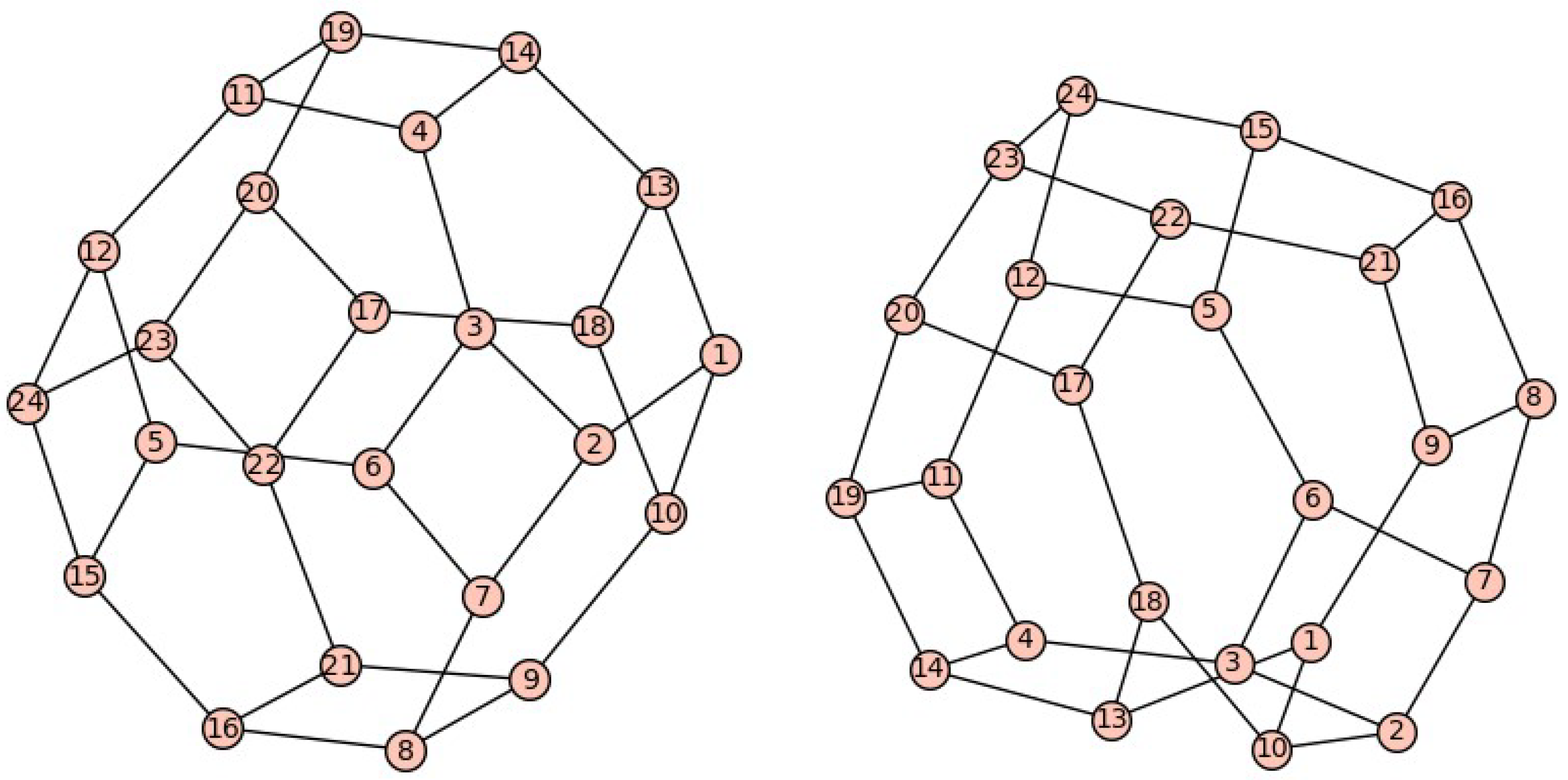
We continue the study [24] of vertex quadrangulations whose obligatory divisor is the complete graph with spectrum and if is bipartite, then its spectrum contains the full spectrum of the cube graph . Note that the existence of a divisor of the graph is a sufficient condition for the presence of the subspectrum in the spectrum of the latter; however, this condition is not necessary in the general case, since there are graphs with such subspectra that are not vertex quadrangulations of simple graphs. The simplest examples are the graphs and themselves, respectively. Moreover, not even every vertex quadrangulation that has eigenvalues has a graph divisor , and the left graph in Figure 2 is an example of this. An example of a nonbipartite vertex quadrangulation of the octahedron graph O, whose spectrum contains only two eigenvalues , is shown in Figure 2 (right), while the spectrum of the bipartite version of shown in Figure 2 (left) has all three eigenvalues of (and ).
In a previous work [24], the question was posed: does the spectrum of an arbitrary unweighted graph include the full spectrum of the tetrahedron graph (complete graph )? As we now know, in the case of nonbipartite graphs , the answer to the question posed depends on the particular graph . The case of bipartite vertex quadrangulations is still less studied.
To proceed, we need to introduce some additional terminology. A straight-ahead walk, or a SAW [36], in the embedded Eulerian graph G always passes from an edge to the opposite edge adjacent to the same vertex; two edges are “opposite” at a vertex of valency in an embedded graph if they are k edges apart in the cyclic ordering (rotation) of the edges at that vertex induced by the embedding. The definition of SAW allows the use of weak embedding, which requires only two conditions to be met: no vertex of the graph coincides on the surface with another vertex or an interior point of an edge. Without loss of generality, we can impose a third condition under which such an embedding is a knot projection of a graph G [36], which prohibits the intersection of more than two edges at one point of the surface. Obviously, if the graph is weakly embedded, then the observer can see each individual vertex on the surface and distinguish between incident edges that project radially from it. We also use the abbreviation SAC [24] to mean a simple cycle of G, along which such a straight-ahead walk (closed simple path) is possible. Below, of particular interest to us are the full vertex covers of G by its cycles that are all SACs.
Let be a decomposition of a simple 4-regular plane graph G into edge-disjoint cycles such that every two adjacent edges on the face belong to different cycles of . Such graphs, called Grötzsch–Sachs graphs, can be viewed as the result of a superposition of simple closed curves in a plane with forbidden tangency [37,38,39,40,41,42,43]. In this text, we will also consider the more general case of not necessarily planar graph G embedded in an arbitrary surface. The benefit of what has been said in the case of a 4-regular graph G is that the above set of cycles is the set of SACs of the graph G (cf. [36] for the general case of an arbitrary SAW).
Now, as promised at the beginning, we need to decide which kind of vertex quadrangulation is of primary interest to us. Let a 4-regular graph G be embedded in some surface. Keeping in mind the definition of opposite edges used in defining SAW above, we can perform vertex quadrangulation in such a way that each pair of opposite edges of G that are incident with a common vertex is attached to a pair of diagonal vertices of the quadrangle that replaced this vertex. Locally, we call this version of vertex quadrangulation consistent, and any other attachment option is inconsistent. But at the same time, we admit the existence of several ways of embedding the graph in one or several different surfaces; in this case, there must be several different consistent quadrangulations. But for us it is only important to know if at least one of them exists. In general, this is not always the case.
Here, we come to the main part of our study.
3. The Main Part
First, we need to recall the famous 2-factor theorem discovered by Julius Petersen (see Theorem 6.2.4, p. 218 in [44]).
Theorem 1
(Petersen). Let G be a regular graph whose degree is an even number, . Then, the edges of G can be partitioned into k edge-disjoint 2-factors.
Of particular interest to us is the following corollary (Corollary 7.1 in [24]).
Corollary 1.
Let G be a 4-regular graph embedded in some surface and having a 2-factor , all of whose components are SACs. Then, G has a complementary (to ) 2-factor , all of whose components are also SACs .
Let be the class of all 4-regular embedded graphs having two complementary SAC factors and satisfying the conditions of Corollary 1 (see [24]); an embedded graph has a consistent vertex quadrangulation. An example is the above-mentioned toroidal graphs [24] (see fragment in Figure 3, top left), which also belong to .
Here, we propose a strengthened version of [24]’s Theorem 10, which now uses the term ‘consistent’ and one additional fact proved in [24] but omitted in the text of the previous version.
Theorem 2.
Let G be a 4-regular simple graph from the class embedded in some surfaces. Then, G has a consistent vertex quadrangulation with divisor , which gives its full spectrum into the spectrum of . Moreover, if G is a bipartite graph, a consistent quadrangulation contains the full spectrum of the cube graph .
Proof.
The assertion that the graph has a divisor is proved in part 2 of the Proof of Theorem 10 in [24]. The other two assertions in Theorem 2 are obvious. □
Theorem 2, in particular, allows us to analyze various special cases of graphs, such as the following. The spectrum of the left graph in Figure 2 contains the full spectrum , but does not have a divisor and, therefore, is not a consistent vertex quadrangulation. It also turns out that the graph O of the octahedron is not a graph from the class at all, since traversing SAW paths in it splits O into three pairwise intersecting SAC 4-cycles. This does not satisfy the definition of the class , since it does not allow finding two complementary spanning graphs and , all of whose components are SAC cycles, as it should be satisfied for the graph .
As we briefly mentioned earlier, the topic of graphs from the class intersects with the topic of certain colorings of such graphs. Of particular interest in graph theory are proper colorings. A coloring of vertices of a graph is called a proper coloring if does not contain any pair of adjacent vertices of the same color. Here, let us recall the upper-left colored graph in Figure 3, which is a good example with which to illustrate the following corollary.
Corollary 2.
Let G be a 4-regular simple graph from and let be its (3-regular) vertex quadrangulation with divisor . Then, there exists a proper coloring ρ of with four colors such that (a) each vertex of any color is adjacent to exactly one vertex of each of the other three colors (but not the same color), and (b) exactly a quarter of the vertices of is colored in each of the colors. The converse of (a) is also true: from the coloring of ρ (as is), it mutually follows that has a divisor .
Proof.
For a surface-embedded graph , the existence of its vertex quadrangulation with divisor follows from Theorem 2. The presence of such a divisor means an equitable partition of the set of all vertices of into four sorts such that a vertex of any sort is adjacent to exactly one vertex each of the other three sorts (but not of the same sort). Since each sort of vertex can be entirely colored in one of four different colors, this proves part (a). The converse statement with respect to (a) follows from the reasoning about the equitable partition of formed by vertices of different colors defined by .
Now show that (b) of Theorem 2 follows from (a). Recall that all vertices of are covered by quadrilaterals. Take any quadrilateral and number its vertices cyclically: . Color vertex 1 red. Since its adjacent vertices must be of different colors, color vertices 2 and 4 green and yellow, respectively. The remaining vertex 3 cannot be colored in any of the three colors already used, since vertices 2 and 4 cannot have two adjacent vertices of the same color. We can only color vertex 3 with another fourth color, e.g., blue. Thus, we establish that according to (a), each quadrilateral of is colored with four different colors. Since the quadrilaterals of cover all its vertices and do not overlap, it is easy to deduce from their strict 4-chromaticity that the number of vertices of each color in is exactly equal to a quarter of their total number. This proves (b), and we arrive at the complete proof. □
Touching upon the topic of graph colorings, it is worth mentioning one more. Here, we use a more general interpretation of definitions than was originally done in [45]. Let be a k-coloring (not necessarily proper) of a graph G. We say that a face f of the graph G embedded in a surface is polychromatic under if all k colors appear in the boundary closed walk of f. The coloring is polychromatic if it is a k-coloring of G such that every face of G is polychromatic; , where g is the girth of graph G (which is equal to the length of the shortest cycle in G). An example of a graph with a polychromatic 4-coloring is shown in Figure 3, upper left.
There is the following fact.
Proposition 1.
Let be a surface-embedded vertex quadrangulation of a graph , and let ρ be a proper 4-coloring of such that every vertex of any color is adjacent to exactly one vertex of each of the other three colors (but not the same color). Then, ρ is a polychromatic coloring.
Proof.
Obviously, each quadrilateral in is 4-colored and hence polychromatic. Each quadrilateral in surface-embedded that has replaced a vertex in G is surrounded by four adjacent faces, each of which shares one edge with the quadrilateral. Number the vertices of the quadrilateral cyclically: 1, 2, 3, 4. Color these vertices red, blue, yellow, and green, respectively. By the method of excluding forbidden options, we find that four other vertices , respectively, adjacent to four vertices of the quadrilateral with the same numbers without a prime, have the colors yellow, green, red, blue. Consider four simple paths in which the central edge is one of the edges of the colored quadrilateral: . Each of these four paths is a part of the corresponding face cycle of one of the four faces adjacent to the quadrangular under consideration. Since the vertices of each of these paths are colored in four different colors, we conclude that the four specified faces are polychromatic faces. Extending our reasoning to all quadrilaterals, we obtain a proof that the coloring of the entire graph is polychromatic. Q.E.D. □
In the definition of the vertex quadrangulation (back in [24]), we missed other possible cases when an underlined 4-regular graph G has multiple edges and/or loops. If we assume that the one-vertex graph with two loops is 4-regular (judging by the total number of lines entering and leaving the vertex), then it can also be quadrangulated, which gives the often-mentioned graph we use, the minimum graph with eigenvalues . And if we take a two-vertex graph with four edges, then after vertex quadrangulation we can obtain the cube graph from it, with eigenvalues .
Any graph embedded in a surface has exactly n quadrangular face cycles if the original graph G does not contain double edges (which can be considered digons, undirected 2-vertex cycles) and has more than n quadrangular cycles if such double edges are present. An example is the vertex quadrangulation of the 4-vertex cycle with double edges , which is the skeletal graph of an octagonal prism with quadrangular faces. This reminds us of the fact that every 3-connected simple planar cubic graph (including with such properties) is a skeletal graph of a convex polyhedron. The last example of the octagonal prism graph is just the case of embedding in a sphere in which each inner face has length or 8.
Recall that, in the general case, the proper 4-coloring of a cubic graph (e.g., ) is not minimal in the number of required colors. Also, not every arbitrarily chosen proper coloring satisfies the Corollary 2 conditions, whereas some of all possible proper colorings may satisfy them. It follows from what has been said that an analysis of a possibly large number of colorings is needed, all of which still need to be found. Meanwhile, we are only interested in the fundamental existence or nonexistence of the required coloring. The question arises: Can we not reduce our problem “as is” to some other problem that is easier to solve? Fortunately, this can be carried out and brought to a simpler determination that some derived graph is or is not properly 4-colorable. The latter no longer requires one to independently compose a computer code, and it is enough to use a ready-made system of symbolic algebraic calculations such as Maple, SageMath, and the like. Now demonstrate this.
For , the power of a simple graph is defined as the graph with the same vertex set V and with an edge between any pair of vertices that are distance at most p away from each other in ; . Thus, in particular, the square of a simple graph Γ is obtained by starting with and adding edges between any two vertices whose distance in is 2.
The chromatic number of a graph is the smallest number of colors needed to color the vertices of in such a way that no two neighboring vertices have the same colors. Moreover, the chromatic number associated with the distance p in the graph Γ [46] is the minimum number of colors that are sufficient to color the vertices of in such a way that any two vertices of located at a distance not greater than p have different colors; .
The following lemma (see [46], p. 422) plays a crucial role in reducing the original problem of coloring the graph to a simpler problem of coloring its square .
Lemma 1.
Let be the the p-th power of a simple graph Γ. Then, .
Before using Lemma 1 in our target case for and , we still need to prove one more technical lemma.
Lemma 2.
Let be the quadrangulation of a 4-regular graph G that has a proper 4-coloring ρ such that every vertex of any color is adjacent to exactly one vertex of each of the other three colors (but not of the same color). Then, ρ is exactly a proper 4-coloring such that no pair of vertices at a distance of from each other is colored with the same color.
Proof.
By the conditions of Lemma 2, no vertex satisfying the coloring can have two adjacent vertices of the same color. Or, equivalently, does not allow any two vertices of the same color in H to have a common neighbor, and hence be at a distance of 2. Since the distance 1 is initially invalid by the definition of a proper coloring, we arrive at a complete proof. □
In the course of the previous discussion, we considered some connections between the chosen graph-theoretic, spectral and chromatic, properties of vertex quadrangulations of 4-regular graphs G. In some cases, some of these properties mutually entail each other, while in others they are only one-sided consequences. We will try to partially reflect what has been said by the following generalizing theorem.
Theorem 3.
Let be the square of a consistent vertex quadrangulation of a 4-regular graph . Then, the following statements are equivalent:
- (a)
- ;
- (b)
- admits its proper 4-coloring ρ such that every vertex of any color is adjacent to exactly one vertex of each of the other three colors (but not of the same color), where exactly a quarter of the vertices of is colored in each of the colors;
- (c)
- has a divisor . Furthermore, these statements imply:
- (d)
- The spectrum includes the full spectrum of the complete graph if , or the full spectrum of the cube if is bipartite (but in the general case, such subspectra can also exist for with );
- (e)
- has polychromatic 4-coloring;
- (f)
- The adjacency matrix of the graph can be reduced by a simultaneous permutation of rows and columns to a block form, where each nondiagonal (nonzero) block is an permutation matrix (having exactly one 1 in each row and column).
Proof.
The 4-coloring we are interested in is the coloring due to the conditions of Lemma 2. Such a coloring exists if and only if . By Lemma 1, , which proves (a) ⇔ (b), wherein the fact that exactly a quarter of the vertices of is colored with each of the colors is proved in Corollary 2. Moreover, from Corollary 2, we obtain (b) ⇔ (c). Using the transitivity of equivalences, we also obtain (a) ⇔ (c). Item (d) follows from Theorem 2 or item (c) of Theorem 3; (e) follows from Proposition 1; (f) follows from the definition of equitable partition of vertices in and points (b) and (c) of Theorem 3. This completes the proof. □
Recall the graphs depicted in Figure 2. The spectrum of contains the full spectrum of the complete graph , while the second graph does not. Calculations using SageMath show that the squares and of both graphs have the chromatic number . This, due to the failure of item (a) of Theorem 3, clearly indicates that both graphs and do not have a divisor , which is indeed the case.
The vertices of the vertex quadrangulation satisfying Theorem 3 can be numbered in such a way that all vertices of the same color (out of four) are numbered consecutively. Then, point (f) of Theorem 3 allows us to represent the adjacency matrix of such a graph as:
where O is an all-zero block, while each block is an permutation matrix.
It is right to ask a question: is an arbitrary adjacency matrix of a graph, which has the block form of the R.H.S. of , always the adjacency matrix of a simple graph ? The answer turns out to be negative. As an example, we studied adjacency matrices in which all blocks are pairwise commuting; and it turned out that the graphs represented by such matrices are, in general, disconnected. Moreover, we generally do not know whether a connected graph with such an adjacency matrix is always a vertex quadrangulation , and not something else. Because of this uncertainty, we a priori admit that even such connected graphs may not be vertex quadrangulations. Thus, there exists the following problem.
Problem 1.
Which set of blocks (permutation matrices) on R.H.S. of will correspond to the adjacency matrix of a connected vertex quadrangulation satisfying Theorem 3?
Despite the general situation, we would like to note that the matrices of a commutative cyclic group (s odd) of matrices can be used as off-diagonal blocks on the R.H.S. of and form the adjacency matrix of a vertex-quadrangulated graph . Consider an example of a adjacency matrix, which can presumably be the adjacency matrix of a quadrangulation of the minimum 4-regular simple graph . The group related to this case consists of the matrices:
Let the off-diagonal blocks on the R.H.S. of be chosen as: .
This gives us the following matrix:
The matrix B actually turns out to be the adjacency matrix (of one of the versions) of the vertex quadrangulation of the complete graph (see Figure 4). This version of the graph illustrates one of the possible (matrix) ways of constructing graphs with divisor . The subsequent cyclic groups (, odd) of matrices can be used in a similar way to construct other such graphs on vertices.
Note that has chromatic number and its square has chromatic number , and the corresponding 4-coloring is unique up to the choice of colors. The corresponding chromatic indices of these graphs are and . An example of the specified coloring of the vertices of the graph in Figure 4 is the one where vertices are colored green; red; yellow; and the vertices are colored blue. A coloring of this type can be easily obtained by first coloring the vertices of one quadrilateral in four different colors, and then, taking into account the conditions for the proper coloring of the vertices in the graph , color all other vertices, gradually moving from colored vertices to adjacent ones. Luckily, as simple as it sounds in words, such an algorithm guarantees a consistent coloring of without a conflict of the chosen colors.
One feature of the vertex coloring in our example is the stable pairs of colors used to color the diagonal vertices of all quadrilaterals in the graph . This is a pair of green and red for the vertices of one diagonal, and a pair of yellow and blue for the vertices of the other diagonal. Accordingly, when two quadrilaterals are connected by an edge, the vertices at the ends of this edge are colored in one pair of diagonal colors, these are also red and green or yellow and blue. That is, all adjacent quadrilaterals are in contact only with their identically 2-colored diagonals, while the corresponding two colors in each garland of concatenated quadrangles in alternate along a garland circle. Taking into account all eight operations of the symmetry group of a regular quadrilateral, there are in total three different colorings of its vertices in four colors. Thus, in a proper coloring of the graph in four colors consistent with the graph , only one of the three types of coloring of all quadrilaterals can be realized. Using the conditions for coloring the square of the graph , we conclude that in order for a 4-colored graph to have a divisor , it is necessary that all quadrilaterals in it be colored the same way.
The chromatic polynomial of the graph (calculated using SageMath) is:
For the number of colorings in four colors this gives 24, which in turn, taking into account 24 possible permutations of colors, corresponds to the only possible way of coloring up to the choice of colors (made when coloring the vertices of the first quadrangle).
At the very beginning, we already noted that, in the case of a nonbipartite vertex quadrangulation of a simple graph G, this can be a graph that either has a divisor or does not. Moreover, in the latter case, the spectrum of the graph may not even contain the full spectrum of the complete graph (recall the right graph in Figure 2). In the case of bipartite graphs , however, no definite assertion has yet been made. Here, we should note that such bipartite graphs include all graphs of truncated 4-regular (before truncation) polyhedra; an example is the left variant of the vertex quadrangulation of the graph O of the octahedron in Figure 2. In the case of bipartite graphs, the original 4-regular graphs (of polyhedra or any other) need not be bipartite themselves.
Since not every graph is a planar graph of a convex polyhedron, we need to remember that any graph can be embedded (drawn), not necessarily uniquely, in some surface of minimum genus g (or some greater genus). A surface and a graph laying on it can be represented in such a way that this surface is divided into (drawn) faces belonging to some complex (nonconvex) polyhedron. Further, we can mentally create tubercles at the locations of the vertices of the polyhedron; after that, it is easy to imagine what will happen as a result of truncating all the corners obtained. What we get is a generalization of the truncation of an ordinary convex polyhedron. In the case when we truncate the vertices of the 4-regular graph G of the polytope, this gives us the vertex quadrangulation of the original 4-regular graph G (see above). One feature of such a graph is reflected in the following lemma:
Lemma 3.
Let G be a 4-regular simple graph embedded in the surface and let be the vertex quadrangulation of the graph G obtained by truncating of the vertices of G on . Then, all the faces of drawn on the same surface that the graph G was drawn are cycles of even length.
Proof.
By definition of the vertex quadrangulation of G (see Figure 1), to each vertex of G corresponds a cycle of an even length 4. Each other facial cycle f of the graph corresponds to the facial cycle of the original graph G; the cycle f of a face in is formed by an alternating sequence of edges, where one edge belonging to the quadrangle alternates with an edge that belonged to the cycle G (before the quadrangulation), and vice versa. Thus, each facial cycle is indeed a cycle of an even length. □
Corollary 3.
Let G be a 4-regular simple bipartite graph embedded in the surface and let be the vertex quadrangulation of the graph G obtained by truncating of the vertices of G on . Then, is a bipartite graph, and all the faces of drawn on the same surface that the graph Gwas drawn are cycles of doubly even lengths .
Let us now turn our attention once again to other possibilities for decorating graphs. In our work (see also [24]), we have so far used vertex quadrangulation, but it is also possible, instead of vertices, to replace each edge with a quadrilateral, whereby each vertex u of an original graph H is replaced by a cycle of length (where d is a degree of u). In so doing, two nonadjacent edges of each quadrilateral are elongated, as is usually done for edges (after all, they replace edges), and two other nonadjacent edges are identified with edges of connected cycles (or, in the general case, a looplike attachment of a quadrilateral to one cycle is allowed). This decoration is called the band decomposition of the original graph, which thus results in a ribbon graph. In a strict topological definition, this sounds as follows. In a ribbon graph [47,48] representation, each vertex of a graph is represented by a topological disk, and each edge is represented by a topological rectangle with two opposite ends glued to the edges of vertex disks (possibly to the same disk as each other).
From a simple comparison of the set of all cubic graphs obtained by the vertex quadrangulation of 4-regular simple graphs and the set of all graphs obtained by band decomposition of any simple graphs, it is clear that both sets consist of the same graphs. Indeed, any graph from either of the two sets is the union of edge-disjoint spanning subgraphs and , where has as components edges, and quadrilaterals. Here, it is important to note that the two decorating operations under consideration produce the same decorated graph from two different simple graphs. That is, if , where is the band decomposition of a graph H, then ; as well as and .
In specific cases, each of the two methods of decorating graphs, band decomposition or vertex quadrangulation, may have certain technical advantages over each other or limitations in their use. In particular (in relation to our context), the first allows one to get the ribbon graph from any simple graph, but the second can only be applied to 4-regular graphs. Also, the image of the corresponding graph in the form of a ribbon graph with long closely spaced parallel lines in the picture can be convenient when considering nanobiotechnology problems, when two such paired lines represent two complementary DNA strands. On the other hand, vertex quadrangulation, in principle, can be done with an arbitrary subset of vertices of valency 4 in the graph (which can also be useful in nanobiotechnology); but the concept of partial band decomposition so far still looks ambiguous.
In this work, we have not yet paid attention to eigenvectors, but we want to make some brief remarks here that may be useful in a wider context. Let be the eigenvector of the adjacency matrix A of an arbitrary simple graph H for the eigenvalue , which implies the equality:
Also, let denote the set containing an arbitrary vertex u and all vertices adjacent to it in H; below, we will identify vertices from with the numbers assigned to these vertices in H. In the case of the eigenvalue , which is of particular interest in our work, leads to an equality for the eigenvector coefficients for the eigenvalue :
where the sum runs over all the coefficients of the vector associated with the vertices from the set . (We do not give a proof for , since this follows simply from the definition of the matrix-by-vector product.)
At the last stage of preparing this text, we learned from the literature that the full spectrum of the tetrahedron graph is always contained in the spectrum of any -cage (which is the cubic graph of a simple polyhedron that has only 3-gons and 6-gons as its faces); see p. 159 in [22] and Theorem in [23]. Moreover, the following sequence of spectra embeddings takes place: , where C denotes a -cage graph, is its leapfrog transformation, and is the double (sequential) leapfrog of C [22] (p. 160). Thus, both and also contain the full spectrum of the tetrahedron graph (complete graph ).
In conclusion, it is worth adding that the connection between the eigenvalue (of multiplicity ) and various structural features of arbitrary simple graphs was studied in [19,21,24,25,26]. In the case of a bipartite graph, one can equivalently talk about the relation of the eigenvalue [26,27] to the same structural features of the graph. Additional examples can be found in the books by Cvetković et al. [30] and Cvetković et al. [49].
The spectral properties of vertex quadrangulations of 4-regular graphs G considered by us and some possible applications of the obtained results (see also [24]) are not the last stage in the study of such graphs with divisor . Research is ongoing.
Funding
This research received no external funding.
Data Availability Statement
Data are contained within the article.
Acknowledgments
The former support of the Ministry of Absorption of the State Israel (through fellowship “Shapiro”) is acknowledged.
Conflicts of Interest
The authors declare no conflicts of interest.
References
- Rouvray, D.H. The Topological Matrix in Quantum Chemistry; Academic Press: London, UK; New York, NY, USA; San Francisco, CA, USA, 1976. [Google Scholar]
- Graovac, A.; Gutman, I.; Trinajstić, N. Topological Approach to the Chemistry of Conjugated Molecules; Springer: Berlin/Heidelberg, Germany, 1977. [Google Scholar]
- Gutman, I.; Polansky, O.E. Mathematical Concepts in Organic Chemistry; Springer: Berlin/Heidelberg, Germany, 1985. [Google Scholar]
- Tang, A.; Kiang, Y.; Jiang, Y.; Yan, G.; Tai, S. Graph Theoretical Molecular Orbitals; Science Press (China): Beijin, China, 1986. [Google Scholar]
- Papulov, Y.G.; Rosenfeld, V.R.; Kemenova, T.G. Molecular Graphs; Tver’ State University: Tver’, Russia, 1990. (In Russian) [Google Scholar]
- Trinajstić, N. Chemical Graph Theory, 2nd ed.; CRC Press, Inc.: Boca Raton, FL, USA, 1992. [Google Scholar]
- Dias, J.R. Molecular Orbital Calculations Using Chemical Graph Theory; Springer: Berlin/Heidelberg, Germany, 1993. [Google Scholar]
- Cvetković, D. Characterizing properties of some graph invariants related to electron charges in the Hückel molecular orbital theory. In Proceedings of the Dimacs Workshop on Discrete Mathematical Chemistry, New Brunswick, NJ, USA, 23–24 March 1998; In DIMACS Series in Discrete Mathematics and Theoretical Computer Science Volume 51. Hansen, P., Fowler, P., Zheng, M., Eds.; American Mathematical Society: Providence, RI, USA, 2000; pp. 79–84. [Google Scholar]
- Diudea, M.V.; Gutman, I.; Lorentz, J. Molecular Topology; “Babeş-Bolyai” University: Cluj-Napoca, Romania, 1999. [Google Scholar]
- Cvetković, D.; Gutman, I. (Eds.) Selected Topics on Applications of Graph Spectra; Matematički Institut SANU (Mathematical Institute SANU): Beograd, Serbia, 2011. [Google Scholar]
- Li, X.; Shi, Y.; Gutman, I. Graph Energy; Springer Science+Business Media, LLC: New York, NY, USA, 2012. [Google Scholar]
- Randić, M.; Nović, M.; Plavšić, D. Solved and Unsolved Problems of Structural Chemistry; CRC Press Taylor & Francis Group: Boca Raton, FL, USA, 2016. [Google Scholar]
- Wagner, S.; Wang, H. Introduction to Chemical Graph Theory; CRC Taylor & Francis Group, LLC: New York, NY, USA, 2019. [Google Scholar]
- Sciriha, I.; Farrugia, A. From Nut Graphs to Molecular Structure and Conductivity; Mathematical Chemistry Monographs (MCM), University of Kragujevac: Kragujevac, Serbia, 2021. [Google Scholar]
- Balasubramanian, K. Enumeration of stable stereo and position isomers of polysubstituted alcohols. Ann. N. Y. Acad. Sci. 1979, 319, 33–36. [Google Scholar] [CrossRef]
- Klein, D.J.; Ryzhov, A.; Rosenfeld, V.R. Permutational isomers on a molecular skeleton with neighbor-excluding ligands. J. Math. Chem. 2009, 45, 892–909. [Google Scholar] [CrossRef]
- Rosenfeld, V.R.; Klein, D.J. Enumeration of substitutional isomers with restrictive mutual positions of ligands. I. Overall counts. J. Math. Chem. 2013, 51, 21–37. [Google Scholar] [CrossRef]
- Rosenfeld, V.R.; Klein, D.J. Enumeration of substitutional isomers with restrictive mutual positions of ligands. II. Counts with restrictions on subsymmetry. J. Math. Chem. 2013, 51, 239–264. [Google Scholar] [CrossRef]
- Došlić, T.; Taheri-Dehkordi, M.; Fath-Tabar, G.H. Packing stars in fullerenes. J. Math. Chem. 2020, 58, 2223–2244. [Google Scholar] [CrossRef]
- Levit, V.E.; Mandrescu, E. The independence polynomial of a graph—A survey. In Proceedings of the 1st International Conference on Algebraic Informatics, Thessaloniki, Greece, 20–23 October 2005; pp. 231–252. [Google Scholar]
- Dias, J.R. Structural origin of specific eigenvalues in chemical graphs of planar molecules. Molecular orbital functional groups. Mol. Phys. 1995, 85, 1043–1060. [Google Scholar] [CrossRef]
- Fowler, P.W.; John, P.E.; Sachs, H. (3,6)-Cages, hexagonal toroidal cages, and their spectra. In Proceedings of the Dimacs Workshop on Discrete Mathematical Chemistry, New Brunswick, NJ, USA, 23–24 March 1998; In DIMACS Series in Discrete Mathematics and Theoretical Computer Science Volume 51. Hansen, P., Fowler, P., Zheng, M., Eds.; American Mathematical Society: Providence, RI, USA, 2000; pp. 139–174. [Google Scholar]
- DeVos, M.; Goddyn, L.; Mohar, B.; Šámal, R. Cayley sum graphs and eigenvalues of (3,6)-fullerenes. J. Combin. Theory B 2009, 99, 358–369. [Google Scholar] [CrossRef]
- Rosenfeld, V.R. The spectrum of the vertex quadrangulation of a 4-regular toroidal graph and beyond. J. Math. Chem. 2021, 59, 1551–1561. [Google Scholar] [CrossRef]
- Rosenfeld, V.R. Covering automorphisms and some eigenvalues of a graph. Discret. Appl. Math. 2023, 331, 25–30. [Google Scholar] [CrossRef]
- Dias, J.R. Algebraic method for solving multiple degenerate eigenvalues in [r]triangulenes. ACS Omega 2023, 8, 18332–18338. [Google Scholar] [CrossRef]
- Randić, M.; El-Basil, S.; King, R.B. On non-symmetry equivalence. Math. Comput. Model. 1988, 11, 641–646. [Google Scholar] [CrossRef]
- Wikipedia, Truncation (Geometry). Available online: https://en.wikipedia.org/wiki/Truncation_%28geometry%29 (accessed on 8 February 2022).
- Diudea, M.V.; Rosenfeld, V.R. The truncation of a cage graph. J. Math. Chem. 2017, 55, 1014–1020. [Google Scholar] [CrossRef]
- Cvetković, D.M.; Doob, M.; Sachs, H. Spectra of Graphs: Theory and Application; Academic Press: New York, NY, USA, 1980. [Google Scholar]
- Wikipedia, Organotin Chemistry. Available online: https://en.wikipedia.org/wiki/Organotin_chemistry (accessed on 30 June 2022).
- Teranishi, Y. Equitable switching and spectra of graphs. Linear Algebra Appl. 2003, 359, 121–131. [Google Scholar] [CrossRef]
- Francis, A.; Smith, D.; Sorensen, D.; Webb, B. Extensions and applications of equitable decompositions for graphs with symmetries. Linear Algebra Appl. 2017, 532, 432–462. [Google Scholar] [CrossRef]
- Rosenfeld, V.R.; Nordahl, T.E. Semigroup theory of symmetry. J. Math. Chem. 2016, 54, 1758–1776. [Google Scholar] [CrossRef]
- Delgado-Friedrichs, O. Analyzing Periodic Nets via the Barycentre Construction. In Lecture on the Inner Workings of Systre Held in Santa Barbara in August 2008, File Systre-Lecture at gavrog.org. Available online: Https://www.bing.com/search?q=Delgado-Friedrichs%2C+O.+Analyzing+periodic+nets+via+the+barycentre+construction.+In+Lecture+on+the+inner+workings+of+Systre+held+in+288+Santa+Barbara+in+August+2008%2C+file+systre-lecture+at+gavrog.org.+Available+online.&qs=n&form=QBRE&sp=-1&lq=1&pq=delgado-friedrichs%2C+o.+analyzing+periodic+nets+via+the+barycentre+construction.+in+lecture+on+the+inner+workings+of+systre+held+in+288+santa+barbara+in+august+2008%2C+file+systre-lecture+at+gavrog.org.+available+online.&sc=0-217&sk=&cvid=650FC2BB6A0C4E318F80CE5F7F98AB63&ghsh=0&ghacc=0&ghpl= (accessed on 22 December 2023).
- Pisanski, T.; Tucker, T.W.; Žitnik, A. Straight-ahead walks in Eulerian graphs. Discret. Math. 2004, 281, 237–246. [Google Scholar] [CrossRef]
- Dobrynin, A.A.; Mel’nikov, L.S. Counterexamples to Grötzsch–Sachs–Koester’s conjecture. Discret. Math. 2006, 306, 591–594. [Google Scholar] [CrossRef]
- Dobrynin, A.A.; Mel’nikov, L.S. Infinite families of 4-chromatic Grötzsch-Sachs graphs. J. Graph Theory 2008, 59, 279–292. [Google Scholar] [CrossRef]
- Dobrynin, A.A.; Mel’nikov, L.S. Two series of edge-4-critical Grötzsch-Sachs graphs generated by four curves in the plane. Sib. Elektron. Mat. Izv. (Siberian Electron. Math. Rep.) 2008, 5, 255–278. [Google Scholar]
- Dobrynin, A.A.; Mel’nikov, L.S. 4-Chromatic edge critical Grötzsch-Sachs graphs. Discret. Math. 2009, 309, 2564–2566. [Google Scholar] [CrossRef]
- Dobrynin, A.A.; Mel’nikov, L.S. 4-Chromatic Koester graphs. Discuss. Math. Graph Theory 2012, 32, 617–627. [Google Scholar] [CrossRef]
- Dobrynin, A.A. A new 4-chromatic edge critical Koester graph. Discret. Math. Lett. 2023, 12, 6–10. [Google Scholar]
- Dobrynin, A.A. Edge 4-critical Koester graph of order 28. Sib. Electron. Math. Rep. 2023, 20, 847–853. Available online: http://semr.math.nsc.ru/v20/n2/p847-853.pdf (accessed on 24 November 2023).
- Lovász, L.; Plummer, M.D. Matching Theory; American Mathematical Society: Providence, RI, USA, 2009. [Google Scholar]
- Horev, E.; Katz, M.J.; Krakovski, R.; Nakamoto, A. Polychromatic 4-coloring of cubic bipartite plane graphs. Discret. Math. 2012, 312, 715–719. [Google Scholar] [CrossRef]
- Kramer, F.; Kramer, H. A survey on the distance-colouring of graphs. Discret. Math. 2008, 308, 422–426. [Google Scholar] [CrossRef]
- Ellis-Monaghan, J.A.; Moffatt, I. “1.1.4 Ribbon Graphs”. In Graphs on Surfaces, Dualities, Polynomials, and Knots; Springer: New York, NY, USA, 2013. [Google Scholar]
- Wikipedia, Ribbon Graph. Available online: https://en.wikipedia.org/wiki/Ribbon_graph#:$\sim$:text=In%20topological%20graph%20theory%2C%20a%20ribbon\%20graph%20is,power%20to%20signed%20rotation%20systems%20or%20graphencoded%20maps (accessed on 11 October 2022).
- Cvetković, D.M.; Doob, M.; Gutman, I.; Torgašev, A. Recent Results in the Theory of Graph Spectra; North-Holland: Amsterdam, The Netherlands, 1988. [Google Scholar]
Figure 1.
A 4-valent vertex (left) and its quadrangulation (right). [Used Pajek].

Figure 2.
Two different vertex quadrangulations: bipartite and nonbipartite of the skeleton graph O of the octahedron. The left graph is also the skeleton graph of the truncated octahedron. The only difference between and is that has edges and , while has edges and instead, which are attached to a common quadrangle . [Used SageMath].

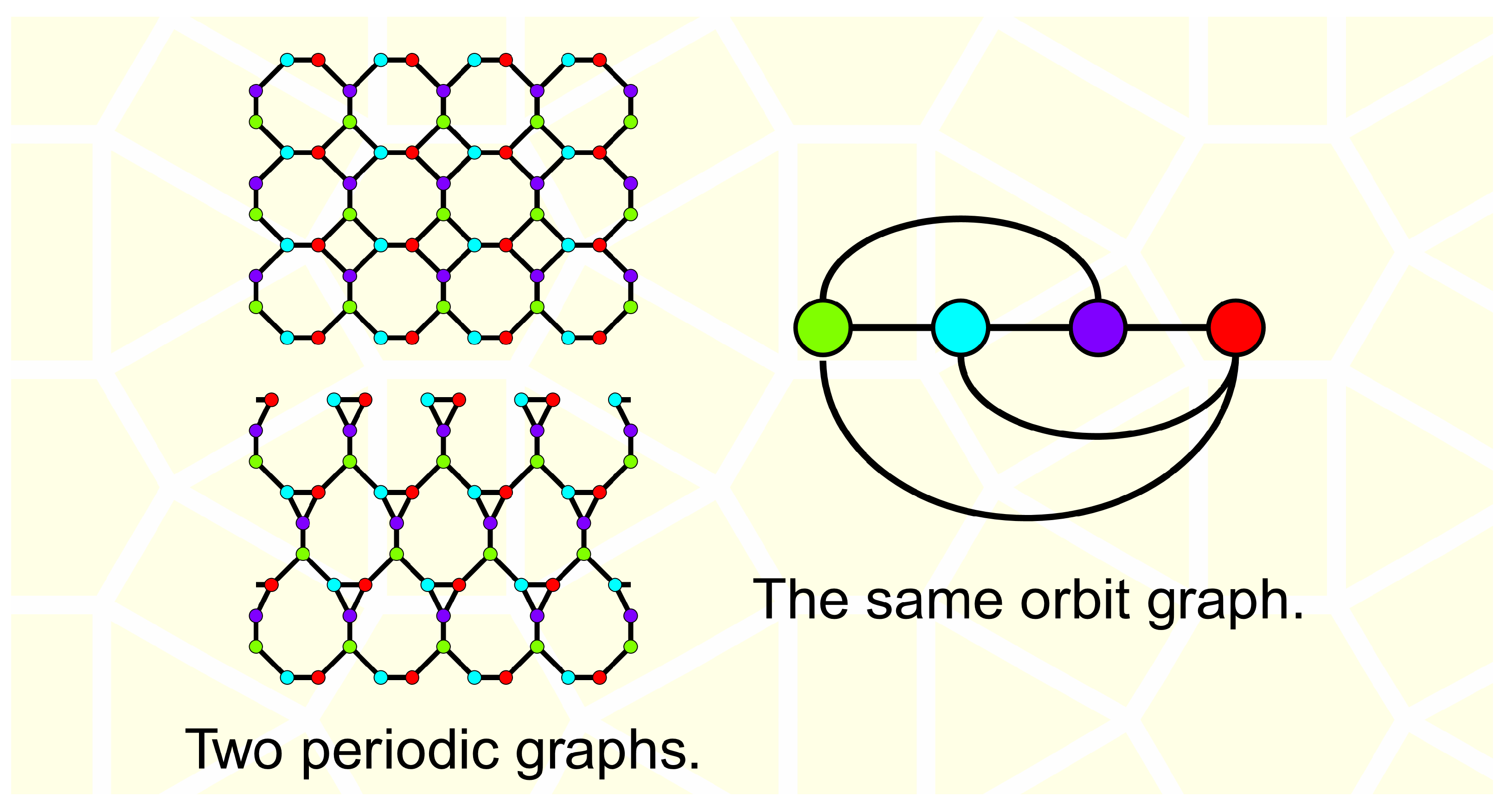
Figure 3.
Fragments of the vertex quadrangulation of the toroidal graph (upper left) and another graph L from [35] (lower left), as well as their common unweighted divisor (right). [Courtesy of O. Delgado-Friedrichs].
Figure 3.
Fragments of the vertex quadrangulation of the toroidal graph (upper left) and another graph L from [35] (lower left), as well as their common unweighted divisor (right). [Courtesy of O. Delgado-Friedrichs].

Figure 4.
A vertex quadrangulation of the complete graph . [Used SageMath].

Disclaimer/Publisher’s Note: The statements, opinions and data contained in all publications are solely those of the individual author(s) and contributor(s) and not of MDPI and/or the editor(s). MDPI and/or the editor(s) disclaim responsibility for any injury to people or property resulting from any ideas, methods, instructions or products referred to in the content. |
© 2024 by the author. Licensee MDPI, Basel, Switzerland. This article is an open access article distributed under the terms and conditions of the Creative Commons Attribution (CC BY) license (https://creativecommons.org/licenses/by/4.0/).
Share and Cite
MDPI and ACS Style
Rosenfeld, V.R. Eigenvalue −1 of the Vertex Quadrangulation of a 4-Regular Graph. Axioms 2024, 13, 72. https://doi.org/10.3390/axioms13010072
AMA Style
Rosenfeld VR. Eigenvalue −1 of the Vertex Quadrangulation of a 4-Regular Graph. Axioms. 2024; 13(1):72. https://doi.org/10.3390/axioms13010072
Chicago/Turabian StyleRosenfeld, Vladimir R. 2024. "Eigenvalue −1 of the Vertex Quadrangulation of a 4-Regular Graph" Axioms 13, no. 1: 72. https://doi.org/10.3390/axioms13010072
Note that from the first issue of 2016, this journal uses article numbers instead of page numbers. See further details here.