Article

On Generalized Class of Bell Polynomials Associated with Geometric Applications

by
Rashad A. Al-Jawfi
1,
Abdulghani Muhyi
2,3,* and
Wadia Faid Hassan Al-shameri
1
1
Department of Mathematics, Faculty of Sciences and Arts, Najran University, Najran 55461, Saudi Arabia
2
Department of Mathematics, Hajjah University, Hajjah, Yemen
3
Department of Mechatronics Engineering, Faculty of Engineering and Smart Computing, Modern Specialized University, Sana’a, Yemen
*
Author to whom correspondence should be addressed.
Axioms 2024, 13(2), 73; https://doi.org/10.3390/axioms13020073
Submission received: 25 November 2023 / Revised: 19 January 2024 / Accepted: 21 January 2024 / Published: 23 January 2024
(This article belongs to the Section Mathematical Analysis)

Abstract

:
In this paper, we introduce a new class of special polynomials called the generalized Bell polynomials, constructed by combining two-variable general polynomials with two-variable Bell polynomials. The concept of the monomiality principle was employed to establish the generating function and obtain various results for these polynomials. We explore certain related identities, properties, as well as differential and integral formulas. Further, specific members within the generalized Bell family—such as the Gould-Hopper-Bell polynomials, Laguerre-Bell polynomials, truncated-exponential-Bell polynomials, Hermite-Appell-Bell polynomials, and Fubini-Bell polynomials—were examined, unveiling analogous outcomes for each. Finally, Mathematica was utilized to investigate the zero distributions of the Gould-Hopper-Bell polynomials.

1. Introduction

Special functions have considerable roles in many branches of mathematics, theoretical physics, and engineering (see [1,2,3]). We realize that various problems in engineering and physics are framed in terms of differential equations, and most of these equations can be investigated by using several families of special polynomials. Further, these special polynomials allow the derivation of various helpful identities in a fairly straightforward way and are useful in introducing new classes of special polynomials. Bell polynomials are some of the most important special polynomials due to their various applications in different mathematical frameworks (see [2,3,4]). Moreover, Bell polynomials play an important role in the studies of water waves which help energy development, mechanical engineering, marine/offshore engineering, hydraulic engineering, etc. [5,6,7,8,9].
Throughout this study, the following notations and definitions are used: N = { 1 , 2 , 3 , . . . } and N 0 = N { 0 } .
The two-variable Bell polynomials (2VBelP) B e l ε ( υ 1 , υ 2 ) [10,11] are defined by
e υ 1 ω e υ 2 ( e ω 1 ) = ε = 0 B e l ε ( υ 1 , υ 2 ) ω ε ε ! .
Taking υ 1 = 0 in generating function (1), we obtain
e υ 2 ( e ω 1 ) = ε = 0 B e l ε ( υ 2 ) ω ε ε ! ,
where B e l ε ( υ 2 ) denotes the classical Bell polynomials [1,12,13].
Taking υ 2 = 1 in generating function (2), we obtain
e ( e ω 1 ) = ε = 0 B e l ε ω ε ε ! ,
where B e l ε denotes the Bell numbers [1,12,13].
Let f ( ω ) = e ( e ω 1 ) 1 . Then the compositional inverse of f ( ω ) is given by
f 1 ( ω ) = log ( 1 + log ( 1 + ω ) ) .
We consider the new type of Bell numbers, which are called Bell numbers of the second kind [14], and are defined by
log ( 1 + log ( 1 + ω ) ) = ε = 1 b e l ε ω ε ε ! .
Note that the classical Bell polynomials satisfy the following relation (see [13])
B e l ε ( υ 2 ) = m = 0 ε S 2 ( ε , m ) υ 2 m ,
where S 2 ( ε , m ) denotes Stirling numbers of the second kind [14] which are defined by
1 m ! ( e ω 1 ) m = ε = m S 2 ( ε , m ) ω ε ε ! .
The two-variable general polynomials (2VGP) G ε ( υ 1 , υ 2 ) [15] are defined by
e υ 1 ω ψ ( υ 2 , ω ) = ε = 0 G ε ( υ 1 , υ 2 ) ω ε ε ! , G 0 ( υ 1 , υ 2 ) = 1 ,
where
ψ ( υ 2 , ω ) = ε = 0 ψ ε ( υ 2 ) ω ε ε ! , ψ 0 ( υ 2 ) 0 .
The idea of monomiality arises from the concept of poweroid proposed by Steffensen [16]. This idea is reformulated and systematically used by Dattoli [17]. According to the monomiality principle [16,17] a given polynomial set ρ ε ( υ ) ( ε N , υ C ) is said to be quasi-monomial, if two operators M ^ , P ^ , called “multiplicative” and “derivative” operators, respectively, can be defined in such a way that
M ^ { ρ ε ( υ ) } = ρ ε + 1 ( υ ) ,
P ^ { ρ ε ( υ ) } = ε ρ ε 1 ( υ ) ,
for all ε N . Also, the operators M ^ and P ^ satisfy the commutation relation
[ P ^ , M ^ ] = P ^ M ^ M ^ P ^ = 1 ^
and thus display the Weyl group structure. If the considered polynomial set { ρ n ( υ ) } ε N is quasi-monomial, its properties can be easily derived from these of the M ^ and P ^ operators. In fact the following holds:
(i)
If M ^ and P ^ have differential realizations, then the polynomials ρ ε ( υ ) satisfy the differential equation
M ^ P ^ { ρ ε ( υ ) } = ε ρ ε ( υ ) .
(ii)
Assuming that ρ 0 ( υ ) = 1 , then the polynomials ρ ε ( υ ) can be explicitly constructed as
ρ ε ( υ ) = M ^ ε { ρ 0 ( υ ) } = M ^ ε { 1 } ,
which gives the series definition of ρ ε ( υ ) .
(iii)
In view of identity (14), the exponential generating function of ρ ε ( υ ) can be written in the form
exp ω M ^ { 1 } = ε = 0 ρ ε ( υ ) ω ε ε ! , | ω | < .
The 2VGP G ε ( υ 1 , υ 2 ) are quasi-monomial [15] with respect to the following operators:
M ^ G = υ 1 + ψ   ( υ 2 , D υ 1 ) ψ ( υ 2 , D υ 1 ) D υ 1 : = υ 1 ; ψ   ( υ 2 , ω ) : = ω ψ ( υ 2 , ω )
and
P ^ G = D υ 1 ,
respectively.
According to the monomiality principle, the 2VGP G ε ( υ 1 , υ 2 ) satisfy the following identities:
M ^ G { G ε ( υ 1 , υ 2 ) } = G ε + 1 ( υ 1 , υ 2 ) ,
P ^ G { G ε ( υ 1 , υ 2 ) } = ε G ε 1 ( υ 1 , υ 2 ) ,
M ^ G P ^ G { G ε ( υ 1 , υ 2 ) } = ε G ε ( υ 1 , υ 2 ) ,
exp ( M ^ G ω ) { 1 } = ε = 0 G ε ( υ 1 , υ 2 ) ω ε ε ! ( | ω | < ) .
The 2VGP family G ε ( υ 1 , υ 2 ) contains a number of significant two-variable special polynomials. Based on suitable choice of the function ψ ( υ 2 , ω ) , various members belonging to the family of two-variable general polynomials G ε ( υ 1 , υ 2 ) can be obtained.
Taking ψ ( υ 2 , ω ) = e υ 2 ω r in generating function (8), gives
e υ 1 t + υ 2 ω r = ε = 0 H ε ( r ) ( υ 1 , υ 2 ) ω ε ε ! ,
where H ε ( r ) ( υ 1 , υ 2 ) are the Gould-Hopper polynomials [18].
Taking ψ ( υ 2 , ω ) = C 0 ( υ 2 ω ) in generating function (8), gives
e υ 1 ω C 0 ( υ 2 ω ) = ε = 0 L ε ( υ 2 , υ 1 ) ω ε ε ! ,
where L ε ( υ 2 , υ 1 ) are the two-variable Laguerre polynomials [19].
Taking ψ ( υ 2 , ω ) = 1 1 υ 2 ω s in generating function (8), gives
1 1 υ 2 ω s e υ 1 ω = ε = 0 e ε ( s ) ( υ 1 , υ 2 ) ω ε ε ! ,
where e ε ( s ) ( υ 1 , υ 2 ) are the two-variable truncated-exponential polynomials of order s [20].
Taking ψ ( υ 2 , ω ) = A ( ω ) e υ 2 ω 2 in generating function (8), gives
A ( ω ) e υ 1 t + υ 2 ω 2 = ε = 0   H A ε ( υ 1 , υ 2 ) ω ε ε ! ,
where   H A ε ( υ 1 , υ 2 ) are the Hermite-Appell polynomials [21].
Taking ψ ( υ 2 , ω ) = 1 1 υ 2 ( e ω 1 ) in generating function (8), gives
e υ 1 ω 1 υ 2 ( e ω 1 ) = ε = 0 F ε ( υ 1 , υ 2 ) ω ε ε ! ,
where F ε ( υ 1 , υ 2 ) are the two-variable Fubini polynomials [22,23].
Recently, numerous researchers have utilized the operational methods together with the monomiality principle [19,20] to establish and investigate new mixed families of special polynomials [24,25,26,27,28,29,30]. Bell polynomials and their diverse generalizations have been densely considered and investigated by many mathematicians. For instance, Duran et al. [10] studied the Bell-based Bernoulli polynomials and their applications. Duran et al. [11] introduced Bell-based Genocchi polynomials and established certain of their properties. Khan et al. [31] defined Bell-based Euler polynomials and investigated some of their properties. Kim et al. [14] investigated a new approach to Bell and poly-Bell numbers and polynomials and discussed some of their properties. Kim et al. [13] investigated some identities of Bell polynomials. Kim et al. [32] studied partially degenerate Bell numbers and polynomials by using umbral calculus and derived some new identities. Kim et al. [25] studied some identities of degenerate Bell polynomials and their properties.
Motivated by the above-mentioned works, in this paper, by combining the two-variable general polynomials with two-variable Bell polynomials, we present a new generalized family of hybrid special polynomials, namely, the generalized Bell polynomials, that is in Definition 1. These polynomials are the most generalizations of the used polynomials, and many other published results are considered as special cases of our current results. The multiplicative and derivative operators, as well as differential equations for this family of polynomials, are also obtained. Next, the series representations and certain other important formulas for the generalized Bell polynomials are derived. Additionally, we obtain partial derivative and integral relations involving these polynomials. Further, certain members related to the generalized Bell polynomials are considered. Finally, we discuss the zero distributions of Gould-Hopper-Bell polynomials.

2. Generalized Bell Polynomials

In this section, we introduce a class of generalized Bell polynomials through generating functions. Then, the generating function is used to derive the related multiplicative and derivative operators, differential equation, and certain series representations.
In generating function (1), replacing υ 1 and υ 2 by the multiplicative operator M ^ G (16) of the 2VGP G ε ( υ 1 , υ 2 ) and z, respectively, gives
exp ( M ^ G ω ) exp ( z ( e ω 1 ) ) = ε = 0 B e l ε ( M ^ G , z ) ω ε ε ! .
Using Equation (21) in the above equation and denoting B e l ε ( M ^ G , z ) by the resultant generalized Bell polynomials (GBelP)   G B e l ε ( υ 1 , υ 2 , z ) , gives
ε = 0 G ε ( υ 1 , υ 2 ) ω ε ε ! exp ( z ( e ω 1 ) ) = ε = 0   G B e l ε ( υ 1 , υ 2 , z ) ω ε ε ! .
Now, utilizing Equation (8) in the above equation, we reach the following definition.
Definition 1.
The generalized Bell polynomials   G B e l ε ( υ 1 , υ 2 , z ) are defined be the following generating function
e υ 1 ω ψ ( υ 2 , ω ) e z ( e ω 1 ) = ε = 0   G B e l ε ( υ 1 , υ 2 , z ) ω ε ε ! .
Remark 1.
Setting υ 1 = 0 in generating relation (29), we obtain
ψ ( υ 2 , ω ) e z ( e ω 1 ) = ε = 0   G B e l ε ( υ 2 , z ) ω ε ε ! ,
where   G B e l ε ( υ 2 , z ) are called two-variable generalized Bell polynomials.
Remark 2.
Setting z = 0 in generating relation (29), we obtain the 2VGP G ε ( υ 1 , υ 2 ) defined by generating function (8).
To show that the generalized Bell polynomials   G B e l ε ( υ 1 , υ 2 , z ) are quasi-monomial, we prove the following results:
Theorem 1.
The generalized Bell polynomials   G B e l ε ( υ 1 , υ 2 , z ) are quasi-monomial with respect to the following multiplicative and derivative operators:
M ^ G B e l = υ 1 + ψ   ( υ 2 , D υ 1 ) ψ ( υ 2 , D υ 1 ) + z e D υ 1
and
P ^ G B e l = D υ 1 ,
respectively.
Proof. 
Obviously, we have
D υ 1 e υ 1 ω ψ ( υ 2 , ω ) e z ( e ω 1 ) = ω e υ 1 ω ψ ( υ 2 , ω ) e z ( e ω 1 ) .
Differentiating Equation (29) partially with respect to ω , gives
υ 1 + ψ   ( υ 2 , ω ) ψ ( υ 2 , ω ) + z e ω ε = 0   G B e l ε ( υ 1 , υ 2 , z ) ω ε ε ! = ε = 0   G B e l ε + 1 ( υ 1 , υ 2 , z ) ω ε ε ! .
Now, using identity (33) and equating the coefficients of like powers of ω in the resultant equation, we have
υ 1 + ψ   ( υ 2 , D υ 1 ) ψ ( υ 2 , D υ 1 ) + z e D υ 1   G B e l ε ( υ 1 , υ 2 , z ) =   G B e l ε + 1 ( υ 1 , υ 2 , z ) ,
which in view of Equation (18) (for   G B e l ε ( υ 1 , υ 2 , z ) ) yields the asserted result (31).
In view of Equation (33), we have
D υ 1 ε = 0   G B e l ε ( υ 1 , υ 2 , z ) ω ε ε ! = ε = 0 ε   G B e l ε 1 ( υ 1 , υ 2 , z ) ω ε ε ! ,
which, upon comparing like powers of ω and utilizing Equation (19) (for   G B e l ε ( υ 1 , υ 2 , z ) ), yield the asserted result (32). □
Theorem 2.
The generalized Bell polynomials   G B e l ε ( υ 1 , υ 2 , z ) satisfy the following differential equation:
υ 1 D υ 1 + ψ   ( υ 2 , D υ 1 ) ψ ( υ 2 , D υ 1 ) D υ 1 + z e D υ 1 D υ 1 ε   G B e l ε ( υ 1 , υ 2 , z ) = 0 .
Proof. 
In view of Equation (20) (for   G B e l ε ( υ 1 , υ 2 , z ) ), utilizing operators (31) and (32), we obtain the asserted result (37). □
Next, by using the generating function (29), we establish some identities and relations including the generalized Bell polynomials.
Theorem 3.
The generalized Bell polynomials   G B e l ε ( υ 1 , υ 2 , z ) satisfy the following series representations:
  G B e l ε ( υ 1 , υ 2 , z ) = κ = 0 ε ε κ G ε κ ( υ 1 , υ 2 ) B e l κ ( z ) ;
  G B e l ε ( υ 1 , υ 2 , z ) = κ = 0 ε ε κ B e l ε κ ( υ 1 , z ) ψ κ ( υ 2 ) ;
  G B e l ε ( υ 1 , υ 2 , z ) = κ = 0 ε ε κ   G B e l κ ( υ 2 , z ) υ 1 ε κ .
Proof. 
In view of generating relations (2) and (8) and Cauchy product rule, generating relation (29) can be written as
ε = 0   G B e l ε ( υ 1 , υ 2 , z ) ω ε ε ! = ε = 0 κ = 0 ε ε κ G ε κ ( υ 1 , υ 2 ) B e l κ ( z ) ω ε ε ! ,
which, upon equating the coefficients of the analogous powers of ω , yields the asserted result (38). Similarly, the assertions (39) and (40) can be proved. □
Theorem 4.
For ε N 0 , we have
  G B e l ε ( υ 1 + u , υ 2 , z + w ) = κ = 0 ε ε κ   G B e l ε κ ( υ 1 , υ 2 , z ) B e l κ ( u , w ) .
Proof. 
Replacing υ 1 by υ 1 + u and z by z + w in (29), then making use of (1) and (29) in the resultant equation, we have
ε = 0   G B e l ε ( υ 1 + u , υ 2 , z + w ) ω ε ε ! = ε = 0 κ = 0 ε κ   G B e l ε κ ( υ 1 , υ 2 , z ) B e l κ ( u , w ) ω ε ε ! ,
which, upon comparing the coefficients of the like powers of ω yields the desired result (42). □
Theorem 5.
For ε N 0 , we have
  G B e l ε ( υ 1 , υ 2 , z ) = 1 2 κ = 0 ε ε κ E κ   G B e l ε κ ( υ 1 + 1 , υ 2 , z ) +   G B e l ε κ ( υ 1 , υ 2 , z ) .
Proof. 
According to generating relation (29), we can write
ε = 0   G B e l ε ( υ 1 + 1 , υ 2 , z ) ω ε ε ! + ε = 0   G B e l ε ( υ 1 , υ 2 , z ) ω ε ε ! = ( e ω + 1 ) ε = 0   G B e l ε ( υ 1 , υ 2 , z ) ω ε ε ! ,
which can be written as
ε = 0   G B e l ε ( υ 1 , υ 2 , z ) ω ε ε ! = 1 2 ε = 0 E ε ω ε ε ! ε = 0   G B e l ε ( υ 1 + 1 , υ 2 , z ) ω ε ε ! + ε = 0   G B e l ε ( υ 1 , υ 2 , z ) ω ε ε ! ,
where E ε denotes the Euler numbers [33]. Finally, using the Cauchy product rule and comparing the like powers of ω in the resultant equation, we obtain (44). □
Theorem 6.
The following implicit summation formula holds true:
  G B e l ε + κ ( σ , υ 2 , z ) = l = 0 ε m = 0 κ ε l κ m ( σ υ 1 ) l + m   G B e l ε + κ l m ( υ 1 , υ 2 , z ) .
Proof. 
Replacing ω by ω + s in (29) and making use of the identity
m = 0 ξ ( m ) ( υ 1 + υ 2 ) m m ! = s , r = 0 ξ ( s + r ) υ 1 s υ 2 r s ! r ! ,
we have
ψ ( υ 2 , ω + s ) e z ( e ω + s 1 ) = e υ 1 ( ω + s ) ε , κ = 0   G B e l ε + κ ( υ 1 , υ 2 , z ) ω ε s κ ε ! κ ! .
Now, replacing υ 1 by σ in (49), then comparing the resultant equation with (49) and simplifying, we obtain
ε , κ = 0   G B e l ε + κ ( σ , υ 2 , z ) ω ε s κ ε ! κ ! = χ = 0 ( ( σ υ 1 ) ( ω + s ) ) χ χ ! ε , κ = 0   G B e l ε + κ ( υ 1 , υ 2 , z ) ω ε s κ ε ! κ ! .
Utilizing identity (48), we obtain
ε , κ = 0   G B e l ε + κ ( σ , υ 2 , z ) ω ε s κ ε ! κ ! = ε , κ = 0 l , m = 0 ε , κ ( σ υ 1 ) l + m   G B e l ε + κ l m ( υ 1 , υ 2 , z ) ω ε s κ l ! m ! ( ε l ) ! ( κ m ) ! ,
which yields the asserted result (47). □
Remark 3.
Taking z = 0 and replacing σ by σ + υ 1 in Equation (47), we obtain
G ε + κ ( σ + υ 1 , υ 2 ) = l = 0 ε m = 0 κ ε l κ m σ l + m G ε + κ l m ( υ 1 , υ 2 ) .

3. Differential and Integral Formulas

In this section, we derive certain differential and integral formulas associated with generalized Bell polynomials   G B e l ε ( υ 1 , υ 2 , z ) .
Theorem 7.
Let ρ , ε N 0 . Then, the following formula holds true:
ρ υ 1 ρ   G B e l ε ( υ 1 , υ 2 , z ) = ε ! ( ε ρ ) !   G B e l ε ρ ( υ 1 , υ 2 , z ) , ε ρ ; 0 , 0 ε < ρ .
Proof. 
Differentiate ρ times generating relation (29) with respect to υ 1 , we have
ε = 0 ρ υ 1 ρ   G B e l ε ( υ 1 , υ 2 , z ) ω ε ε ! = ω ρ e υ 1 ω ψ ( υ 2 , ω ) e z ( e ω 1 ) = ε = 0   G B e l ε ( υ 1 , υ 2 , z ) ω ε + ρ ε ! = ε = ρ   G B e l ε ρ ( υ 1 , υ 2 , z ) ω ε ( ε ρ ) ! ,
which, on simplifying then comparing the coefficients of ω ε ε ! on both sides yield the asserted result (53). □
Remark 4.
When ρ = 1 in (53), we obtain
υ 1   G B e l ε ( υ 1 , υ 2 , z ) = ε   G B e l ε 1 ( υ 1 , υ 2 , z ) .
Theorem 8.
Let κ , ε N 0 . Then, the following formula holds true:
z   G B e l ε ( υ 1 , υ 2 , z ) = ε κ = 0 ε 1 ε 1 κ   G B e l ε κ 1 ( υ 1 , υ 2 , z ) κ + 1 .
Proof. 
Differentiate generating relation (29) with respect to z, we have
ε = 0 z   G B e l ε ( υ 1 , υ 2 , z ) ω ε ε ! = ( e ω 1 ) ε = 0   G B e l ε ( υ 1 , υ 2 , z ) ω ε ε ! = ε = 0 ω ε + 1 ( ε + 1 ) ! ε = 0   G B e l ε ( υ 1 , υ 2 , z ) ω ε ε ! ,
which, upon simplifying and using the Cauchy product rule yields the desired result (56). □
Similarly, we can prove the following results.
Theorem 9.
Let κ , ε N 0 . Then, the following formulas hold true:
z   G B e l ε ( υ 1 , υ 2 , z ) = κ = 0 ε ε κ   G B e l κ ( υ 1 , υ 2 , z ) G ε κ ( υ 1 , υ 2 ) B e l κ ( z ) ;
z   G B e l ε ( υ 1 , υ 2 , z ) = κ = 0 ε ε κ   G B e l κ ( υ 1 , υ 2 , z ) B e l ε κ ( υ 1 , z ) ψ κ ( υ 2 ) ;
z   G B e l ε ( υ 1 , υ 2 , z ) = κ = 0 ε ε κ   G B e l κ ( υ 1 , υ 2 , z )   G B e l m ( υ 2 , z ) υ 1 ε κ ;
  G B e l ε ( υ 1 , υ 2 , z ) = κ = 0 ε + 1 ε + 1 κ B κ z   G B e l ε κ + 1 ( υ 1 , υ 2 , z ) ,
where B κ denotes the Bernoulli numbers [33].
Theorem 10.
The following formula holds true:
u u + w   G B e l ε ( υ 1 , υ 2 , z ) d υ 1 = 1 ε + 1   G B e l ε + 1 ( u + w , υ 2 , z )   G B e l ε + 1 ( u , υ 2 , z ) .
Proof. 
Integrating both sides of generating relation (29) with respect to υ 1 , we have
ε = 0 u u + w   G B e l ε ( υ 1 , υ 2 , z ) d υ 1 ω ε ε ! = 1 ω e ( u + w ) ω ψ ( υ 2 , ω ) e z ( e ω 1 ) e u ω ψ ( υ 2 , ω ) e z ( e ω 1 ) = 1 ω ε = 0   G B e l ε ( u + w , υ 2 , z ) ω ε ε ! ε = 0   G B e l ε ( u , υ 2 , z ) ω ε ε ! ,
which yields the assertion in (62). □
Similarly, we can prove the following results.
Theorem 11.
The following formulas hold true:
u u + w   G B e l ε ( υ 1 , υ 2 , z ) d υ 1 = 1 ε + 1 κ = 0 ε + 1 ε + 1 κ B e l κ ( z ) G ε κ + 1 ( u + w , υ 2 ) G ε κ + 1 ( u , υ 2 ) ;
u u + w   G B e l ε ( υ 1 , υ 2 , z ) d υ 1 = 1 ε + 1 κ = 0 ε + 1 ε + 1 κ ψ κ ( υ 2 ) B e l ε κ + 1 ( u + w , z ) B e l ε κ + 1 ( u , z ) ;
u u + w   G B e l ε ( υ 1 , υ 2 , z ) d υ 1 = 1 ε + 1 κ = 0 ε + 1 ε + 1 κ   G B e l κ ( υ 2 , z ) ( u + w ) ε κ + 1 u ε κ + 1 .
In the next section, certain special members of the generalized Bell polynomials   G B e l ε ( υ 1 , υ 2 , z ) are considered.

4. Special Members

Here, we present some special hybrid members of the generalized Bell polynomials   G B e l ε ( υ 1 , υ 2 , z ) . The obtained results in the previous sections are used to investigate the corresponding results for these members.
I. Taking ψ ( υ 2 , ω ) = e υ 2 ω r in generating function (29), gives
e υ 1 t + υ 2 ω r + z ( e ω 1 ) = ε = 0   H ( r ) B e l ε ( υ 1 , υ 2 , z ) ω ε ε ! ,
where   H ( r ) B e l ε ( υ 1 , υ 2 , z ) are called the Gould-Hopper-Bell polynomials. Certain corresponding results related to these polynomials are mentioned in Table 1.
II. Taking ψ ( υ 2 , ω ) = C 0 ( υ 2 ω ) in generating function (29), gives
e υ 1 ω C 0 ( υ 2 ω ) e z ( e ω 1 ) = ε = 0   L B e l ε ( υ 1 , υ 2 , z ) ω ε ε ! ,
where   L B e l ε ( υ 1 , υ 2 , z ) are called the Laguerre-Bell polynomials. Certain corresponding results related to these polynomials are mentioned in Table 2.
III. Taking ψ ( υ 2 , ω ) = 1 1 υ 2 ω s in generating function (29), gives
1 1 υ 2 ω s e υ 1 ω + z ( e ω 1 ) = ε = 0   e ( s ) B e l ε ( υ 1 , υ 2 , z ) ω ε ε ! ,
where   e ( s ) B e l ε ( υ 1 , υ 2 , z ) are called the truncated-exponential-Bell polynomials of order s. Certain corresponding results related to these polynomials are mentioned in Table 3.
IV. Taking ψ ( υ 2 , ω ) = A ( ω ) e υ 2 ω 2 in generating function (29), gives
A ( ω ) e υ 1 t + υ 2 ω 2 + z ( e ω 1 ) = ε = 0     H A B e l ε ( υ 1 , υ 2 , z ) ω ε ε ! ,
where     H A B e l ε ( υ 1 , υ 2 , z ) are called the Hermite-Appell-Bell polynomials. Certain corresponding results related to these polynomials are mentioned in Table 4.
V. Taking ψ ( υ 2 , ω ) = 1 1 υ 2 ( e ω 1 ) in generating function (29), gives
e υ 1 ω 1 υ 2 ( e ω 1 ) e z ( e ω 1 ) = ε = 0   F B e l ε ( υ 1 , υ 2 , z ) ω ε ε ! ,
where   F B e l ε ( υ 1 , υ 2 , z ) are called the Fubini-Bell polynomials. Certain corresponding results related to these polynomials are mentioned in Table 5.

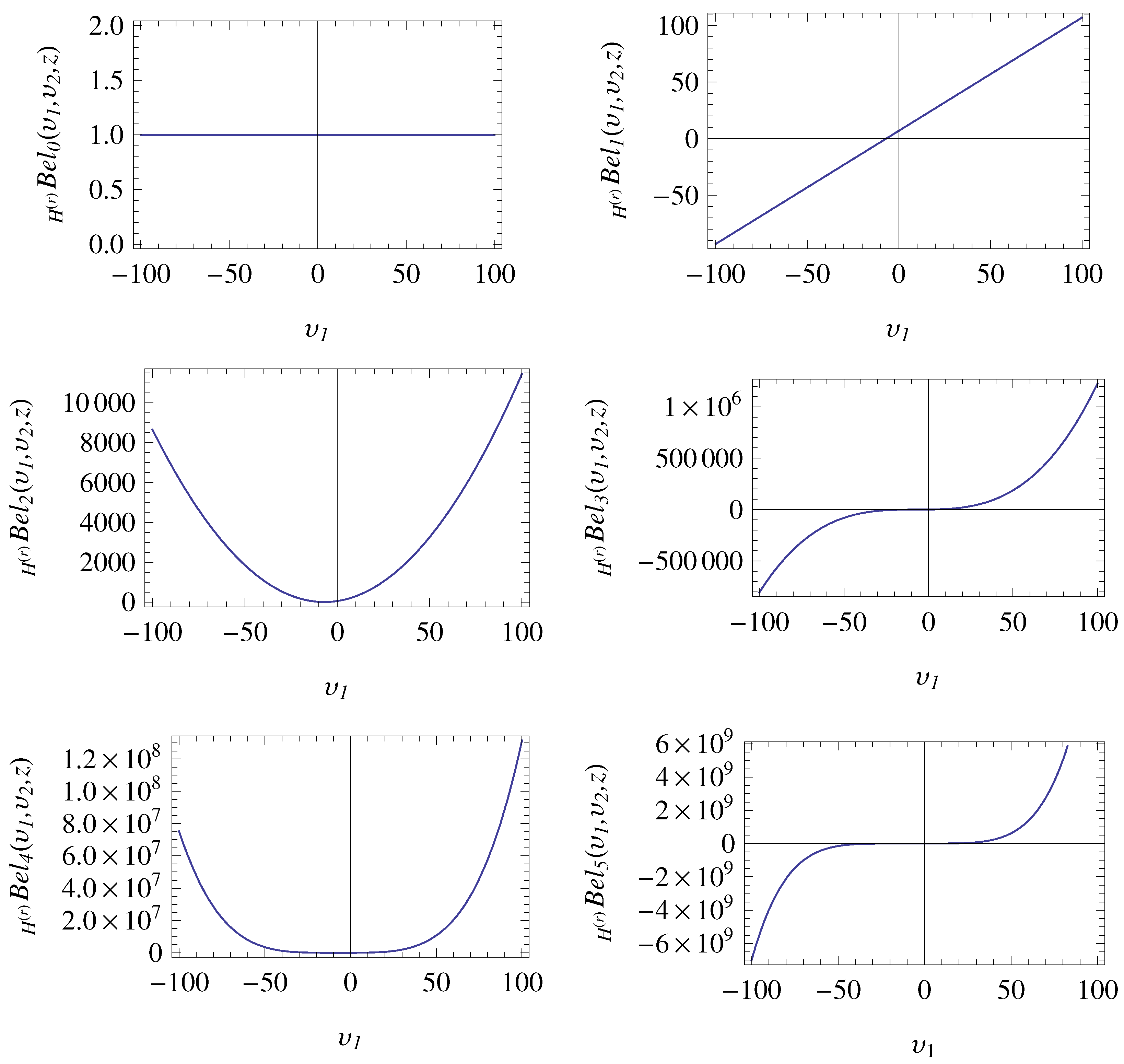
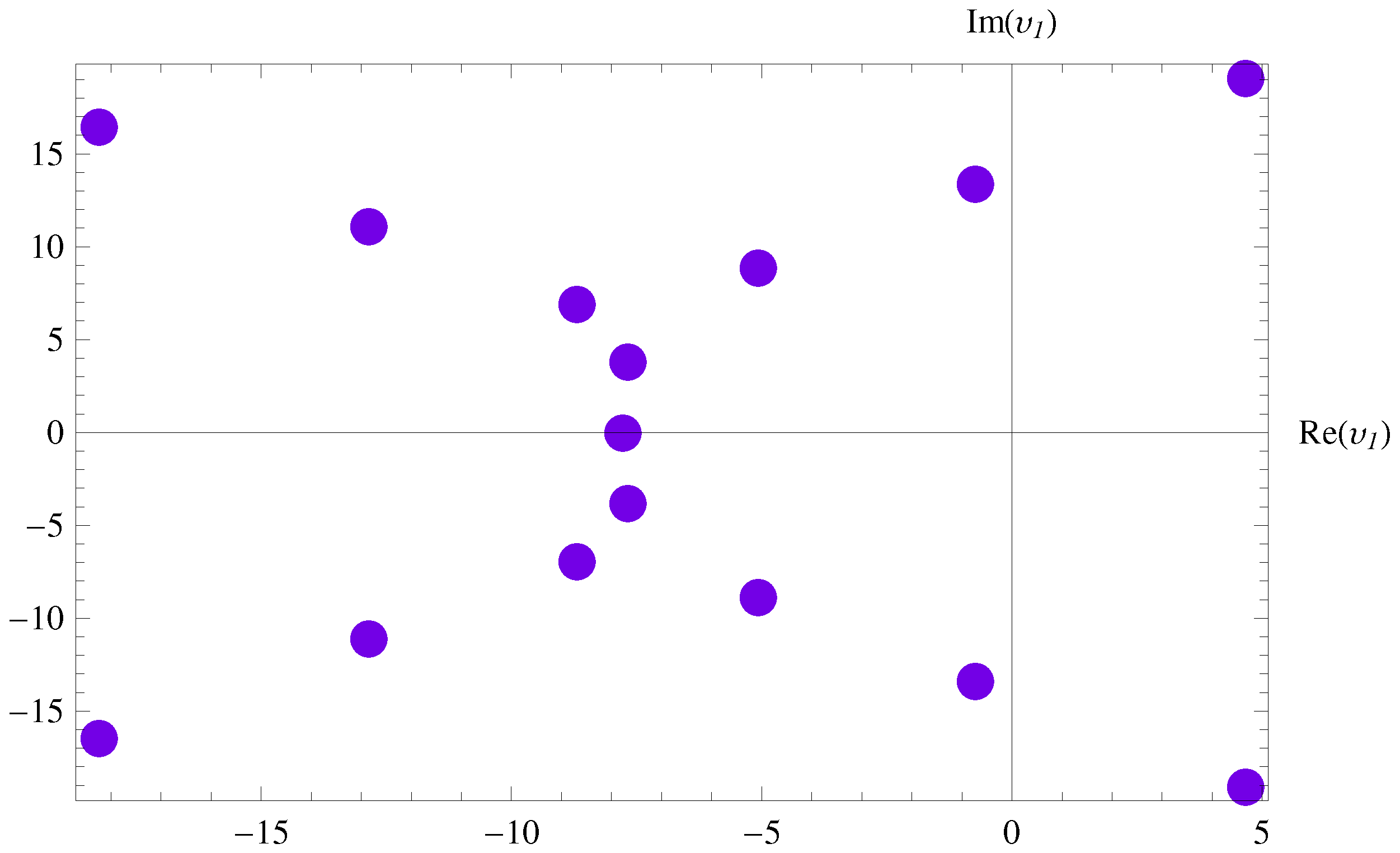
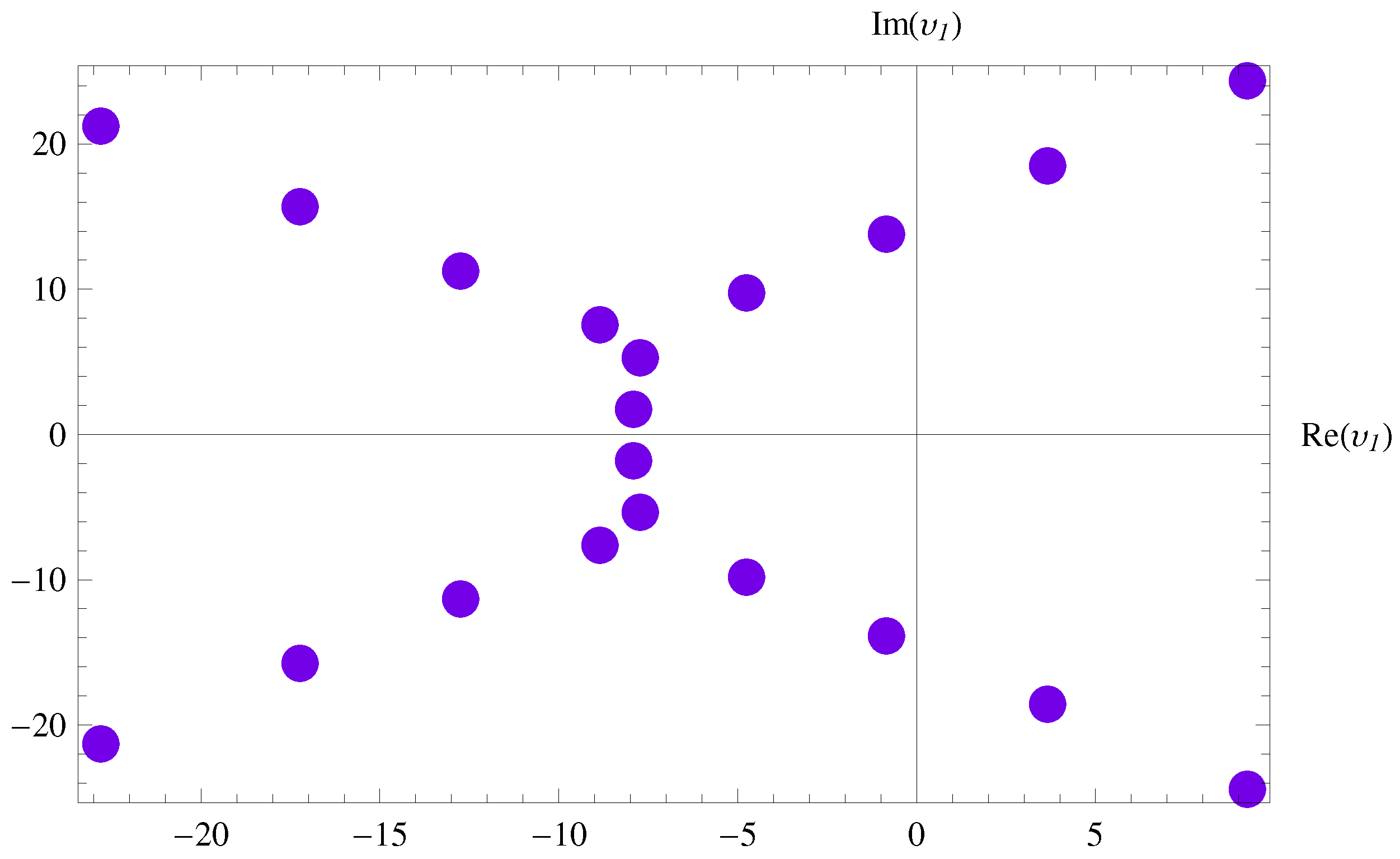
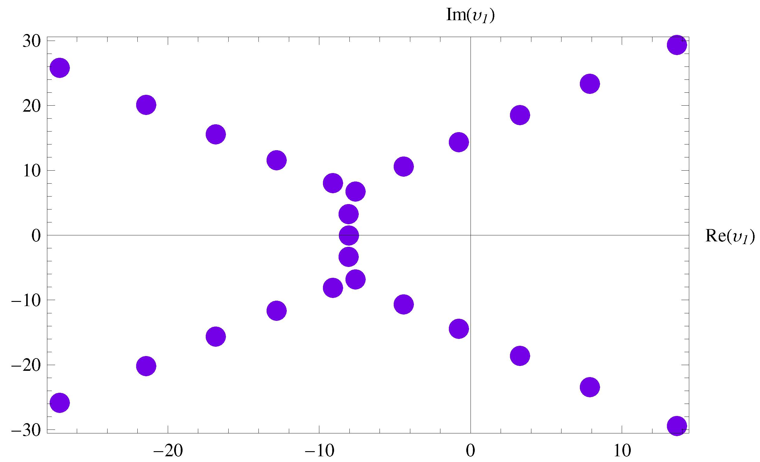
5. Applications in Computer Modeling

Here, we discuss zero distributions and show some graphical representations of the Gould-Hopper-Bell polynomials (GHBelP)   H ( r ) B e l ε ( υ 1 , υ 2 , z ) for some values of the parameters and indices.
In view of (67), the first few members of the GHBelP   H ( r ) B e l ε ( υ 1 , υ 2 , z ) for r = 4 are:
  H ( r ) B e l 0 ( υ 1 , υ 2 , z ) = 1 ,   H ( r ) B e l 1 ( υ 1 , υ 2 , z ) = υ 1 + z ,   H ( r ) B e l 2 ( υ 1 , υ 2 , z ) = υ 1 2 + z + 2 υ 1 z + z 2 ,   H ( r ) B e l 3 ( υ 1 , υ 2 , z ) = υ 1 3 + z + 3 υ 1 z + 3 υ 1 2 z + 3 z 2 + 3 υ 1 z 2 + z 3 υ 1 z 2 + z 3 ,   H ( r ) B e l 4 ( υ 1 , υ 2 , z ) = υ 1 4 + 24 υ 2 + z + 4 υ 1 z + 6 υ 1 2 z + 4 υ 1 3 z + 7 z 2 + 12 υ 1 z 2 + 6 υ 1 2 z 2 + 6 z 3 + 4 υ 1 z 3 + z 4 ,   H ( r ) B e l 5 ( υ 1 , υ 2 , z ) = υ 1 5 + 120 υ 1 υ 2 + z + 5 υ 1 z + 10 υ 1 2 z + 10 υ 1 3 z + 5 υ 1 4 z + 120 υ 2 z + 15 z 2 + 35 υ 1 z 2 + 30 υ 1 2 z 2 + 10 υ 1 3 z 2 + 25 z 3 + 30 υ 1 z 3 + 10 υ 1 2 z 3 + 10 z 4 + 5 υ 1 z 4 + z 5 .
The graphs of these members for r = 4 , υ 2 = 6 and z = 7 are shown in Figure 1.
The zero distribution of some members of the GHBelP   H ( r ) B e l ε ( υ 1 , υ 2 , z ) , i.e., for ε = 5 , 10 , 15 , 20 , 25 , 30 , 35 , 40 are shown in Figure 2, Figure 3, Figure 4, Figure 5, Figure 6, Figure 7, Figure 8 and Figure 9.
Remark 5.
We observed that the GHBelP   H ( r ) B e l ε ( υ 1 , υ 2 , z ) for r = 4 , υ 2 = 6 , z = 7 of degree ε has ε zeros and these zeros have the following properties:
1. 
If ε is odd, the GHBelP   H ( r ) B e l ε ( υ 1 , υ 2 , z ) has one real zero and ε 1 complex zeros.
2. 
If ε is even, the GHBelP   H ( r ) B e l ε ( υ 1 , υ 2 , z ) has ε complex zeros.
3. 
The zeros of the GHBelP   H ( r ) B e l ε ( υ 1 , υ 2 , z ) are symmetric with respect to the real axis.
The 3D structure of zeros distribution of GHBelP   H ( r ) B e l ε ( υ 1 , 6 , 7 ) is presented in Figure 10.

6. Conclusions

Recently, the hybrid forms of special polynomials and numbers have gained worthy consideration by various researchers. The operational methods developed within the context of the monomiality principle offer the opportunity to establish new classes of hybrid special polynomials. In this paper, we introduced a new class of hybrid special polynomials, namely, the generalized Bell polynomials. The generating function and diverse results for these polynomials are obtained. We explored certain related identities, properties, as well as differential and integral formulas. Further, certain special members of the generalized Bell family—such as the Gould-Hopper-Bell polynomials, Laguerre-Bell polynomials, truncated-exponential-Bell polynomials, Hermite-Appell-Bell polynomials, and Fubini-Bell polynomials—were examined, unveiling analogous outcomes for each. Our current results are the most generalizations of the used polynomials, and many other published results are considered as special cases of our current results. Furthermore, we used Mathematica to examine the zeros of Gould-Hopper-Bell polynomials and show that these zeros are symmetric about the real axis, see Figure 2, Figure 3, Figure 4, Figure 5, Figure 6, Figure 7, Figure 8 and Figure 9. The 3D distribution of the zeros can be also viewed in the graph which is given in Figure 10. The integral equations containing these types of special polynomials and related applications can be investigated in further studies.

Author Contributions

Conceptualization, A.M., R.A.A.-J. and W.F.H.A.-s.; software, A.M.; validation, R.A.A.-J. and W.F.H.A.-s.; investigation, A.M.; resources, A.M.; writing—original draft preparation, A.M.; writing—review and editing, A.M.; visualization, W.F.H.A.-s.; supervision, R.A.A.-J. All authors have read and agreed to the published version of the manuscript.

Funding

This work was supported by the Deanship of Scientific Research at Najran University, under the Distinguished Research Funding program grant code (NU/DRP/SERC/12/4).

Informed Consent Statement

Not applicable.

Data Availability Statement

Data are contained within the article.

Acknowledgments

The authors are thankful to the Deanship of Scientific Research at Najran University for funding this work under the Distinguished Research Funding program grant code (NU/DRP/SERC/12/4).

Conflicts of Interest

The authors declare no conflict of interest.

References

  1. Bell, E.T. Exponential polynomials. Ann. Math. 1934, 35, 258–277. [Google Scholar] [CrossRef]
  2. Benbernou, S.; Gala, S.; Ragusa, M.A. On the regularity criteria for the 3D magnetohydrodynamic equations via two components in terms of BMO space. Math. Methods Appl. Sci. 2014, 37, 2320–2325. [Google Scholar] [CrossRef]
  3. Boas, R.B.; Buck, R.C. Polynomial Expansions of Analytic Functions; Springer: Berlin, Germany, 2013. [Google Scholar]
  4. Sándor, J.; Crstici, B. Handbook of Number Theory; Kluwer Academic Publishers: Dordrecht, The Netherlands, 2004; Volume II. [Google Scholar]
  5. Gao, X.-Y.; Guo, Y.-J.; Shan, W.-R. Beholding the shallow water waves near an ocean beach or in a lake via a Boussinesq-Burgers system. Chaos Soliton. Fract. 2021, 147, 110875. [Google Scholar] [CrossRef]
  6. Gao, X.-Y.; Guo, Y.-J.; Shan, W.-R. Bilinear forms through the binary Bell polynomials, N solitons and Bäcklund transformations of the Boussinesq–Burgers system for the shallow water waves in a lake or near an ocean beach. Commun. Theor. Phys. 2020, 72, 095002. [Google Scholar] [CrossRef]
  7. Gao, X.-Y.; Guo, Y.-J.; Shan, W.-R. Scaling transformation, hetero-Backlund transformation and similarity reduction on a (2+1)-dimensional generalized variable-coefficient Boiti-Leon-Pempinelli system for water waves. Rom. Rep. Phys. 2021, 73, 111. [Google Scholar]
  8. Gao, X.-Y.; Guo, Y.-J.; Shan, W.-R. Looking at an open sea via a generalized (2+1)-dimensional dispersive long-wave system for the shallow water: Scaling transformations, hetero-Bäcklund transformations, bilinear forms and N solitons. Eur. Phys. J. Plus 2021, 136, 893. [Google Scholar] [CrossRef]
  9. Li, J.-C.; Nie, B.-C. A few frontier issues in ocean engineering mechanics. China Ocean Eng. 2021, 35, 1–11. [Google Scholar] [CrossRef]
  10. Duran, U.; Araci, S.; Acikgoz, M. Bell-based Bernoulli polynomials with applications. Axioms 2021, 10, 29. [Google Scholar] [CrossRef]
  11. Duran, U.; Acikgoz, M. Bell-based Genocchi polynomials. In Proceedings of the International Conference on Applied Analysis and Mathematical Modeling (ICAAMM21), Istanbul, Turkey, 11–13 June 2021. [Google Scholar]
  12. Carlitz, L. Some remarks on the Bell numbers. Fibonacci Quart. 1980, 18, 66–73. [Google Scholar]
  13. Kim, D.S.; Kim, T. Some identities of Bell polynomials. Sci. China Math. 2015, 58, 2095–2104. [Google Scholar] [CrossRef]
  14. Kim, T.; Kim, D.S.; Dolgy, V.; Kim, H.K.; Lee, H. A new approach to Bell and poly-Bell numbers and polynomials. AIMS Math. 2021, 7, 4004–4016. [Google Scholar] [CrossRef]
  15. Khan, S.; Raza, N. General-Appell polynomials within the context of monomiality principle. Int. J. Anal. 2013, 3013, 328032. [Google Scholar] [CrossRef]
  16. Steffensen, J.F. The poweriod, an extension of the mathematical notion of power. Acta Math. 1941, 73, 333–366. [Google Scholar] [CrossRef]
  17. Dattoli, G. Hermite–Bessel and Laguerre–Bessel functions: A by-product of the monomiality principle. In Advanced Special Functions and Applications, Proceedings of the First Melfi School on Advanced Topics in Mathematics and Physics, Melfi, Italy, 9–12 May 1999; Aracne: Rome, Italy, 2000; Volume 1, pp. 147–164. [Google Scholar]
  18. Gould, H.W.; Hopper, A.T. Operational formulas connected with two generalizations of Hermite polynomials. Duke. Math. J. 1962, 29, 51–63. [Google Scholar] [CrossRef]
  19. Cocolicchio, D.; Dattoli, G.; Srivastava, H.M. Advanced Special Functions and Applications. In Proceedings of the First Melfi School on Advanced Topics in Mathematics and Physics, Melfi, Italy, 9–12 May 1999; Aracne Editrice: Rome, Italy, 2000. [Google Scholar]
  20. Dattoli, G.; Migliorati, M.; Srivastava, H.M. A class of Bessel summation formulas and associated operational methods. Fract. Calc. Appl. Anal. 2004, 7, 169–176. [Google Scholar]
  21. Khan, S.; Yasmin, G.; Khan, R.; Hassan, N.A.M. Hermite-based Appell polynomials: Properties and applications. J. Math. Anal. Appl. 2009, 351, 756–764. [Google Scholar] [CrossRef]
  22. Kilar, N.; Simsek, Y. A new family of Fubini type numbers and polynomials associated with Apostol-Bernoulli numbers and polynomials. J. Korean Math. Soc. 2017, 54, 1605–1621. [Google Scholar]
  23. Srivastava, H.M.; Srivastava, R.; Muhyi, A.; Yasmin, G.; Islahi, H.; Araci, S. Construction of a new family of Fubini-type polynomials and its applications. Adv. Differ. Equ. 2021, 2021, 36. [Google Scholar] [CrossRef]
  24. Khan, S.; Raza, N.; Ali, M. Finding mixed families of special polynomials associated with Appell sequences. J. Math. Anal. Appl. 2017, 447, 398–418. [Google Scholar] [CrossRef]
  25. Kim, T.; Kim, D.S.; Kim, H.Y.; Kwon, J. Some identities of degenerate Bell polynomials. Mathematics 2020, 8, 40. [Google Scholar] [CrossRef]
  26. Muhyi, A. A new class of Gould-Hopper-Eulerian-type polynomials. Appl. Math. Sci. Eng. 2022, 30, 283–306. [Google Scholar] [CrossRef]
  27. Srivastava, H.M.; Araci, S.; Khan, W.A.; Acikgoz, M. A note on the truncated-exponential based Apostol-type polynomials. Symmetry 2019, 11, 538. [Google Scholar] [CrossRef]
  28. Srivastava, H.M.; Özarslan, M.A.; Yılmaz, B. Some families of differential equations associated with the Hermite-based Appell polynomials and other classes of Hermite-based polynomials. Filomat 2014, 28, 695–708. [Google Scholar] [CrossRef]
  29. Yasmin, G.; Muhyi, A. Certain results of hybrid families of special polynomials associated with Appell sequences. Filomat 2019, 33, 3833–3844. [Google Scholar] [CrossRef]
  30. Yasmin, G. Some properties of Legendre–Gould Hopper polynomials and operational methods. J. Math. Anal. Appl. 2014, 413, 84–99. [Google Scholar] [CrossRef]
  31. Khan, N.; Husain, S. Analysis of Bell Based Euler Polynomials and Their Application. Int. J. Appl. Comput. Math. 2021, 7, 195. [Google Scholar] [CrossRef]
  32. Kim, T.; Kim, D.S.; Kwon, H.-I.; Rim, S.-H. Some identities for umbral calculus associated with partially degenerate Bell numbers and polynomials. J. Nonlinear Sci. Appl. 2017, 10, 2966–2975. [Google Scholar] [CrossRef]
  33. Rainville, E.D. Special Functions; Reprint of 1960 First Edition; Chelsea Publishing Co.: Bronx, NY, USA, 1971. [Google Scholar]
Figure 1. Graphs of   H ( r ) B e l ε ( υ 1 , υ 2 , z ) , for ε = 0 , 1 , 2 , 3 , 4 , 5 .
Axioms 13 00073 g001
Figure 2. Zero distribution of   H ( r ) B e l 5 ( υ 1 , 6 , 7 ) .
Axioms 13 00073 g002
Figure 3. Zero distribution of   H ( r ) B e l 10 ( υ 1 , 6 , 7 ) .
Axioms 13 00073 g003
Figure 4. Zero distribution of   H ( r ) B e l 15 ( υ 1 , 6 , 7 ) .
Axioms 13 00073 g004
Figure 5. Zero distribution of   H ( r ) B e l 20 ( υ 1 , 6 , 7 ) .
Axioms 13 00073 g005
Figure 6. Zero distribution of   H ( r ) B e l 25 ( υ 1 , 6 , 7 ) .
Axioms 13 00073 g006
Figure 7. Zero distribution of   H ( r ) B e l 30 ( υ 1 , 6 , 7 ) .
Axioms 13 00073 g007
Figure 8. Zero distribution of   H ( r ) B e l 35 ( υ 1 , 6 , 7 ) .
Axioms 13 00073 g008
Figure 9. Zero distribution of   H ( r ) B e l 40 ( υ 1 , 6 , 7 ) .
Axioms 13 00073 g009
Figure 10. Zero distribution of   H ( r ) B e l ε ( υ 1 , 6 , 7 ) = 0 . This figure shows the 3D plot of the zeros of Gould-Hopper-Bell polynomials   H ( r ) B e l ε ( υ 1 , υ 2 , z ) for ε = 5 , 10 , 15 , 20 , 25 , 30 , 35 , 40 , υ 2 = 6 and z = 7 .
Axioms 13 00073 g010
Table 1. Results for Gould-Hopper-Bell polynomials   H ( r ) B e l ε ( υ 1 , υ 2 , z ) .
Multiplicative and M ^ G H B e l = υ 1 + r υ 2 D υ 1 r 1 + z e D υ 1 , P ^ G H B e l : = D υ 1
derivative operators
Differential equation υ 1 D υ 1 + r υ 2 D υ 1 r + z e D υ 1 D υ 1 ε   H ( r ) B e l ε ( υ 1 , υ 2 , z ) = 0
Identities and   H ( r ) B e l ε ( υ 1 , υ 2 , z ) = κ = 0 ε ε κ H ε κ ( r ) ( υ 1 , υ 2 ) B e l κ ( z )
relations   H ( r ) B e l ε ( υ 1 + u , υ 2 , z + w ) = κ = 0 ε ε κ   H ( r ) B e l ε κ ( υ 1 , υ 2 , z ) B e l κ ( u , w )
  H ( r ) B e l ε ( υ 1 , υ 2 , z ) = 1 2 κ = 0 ε ε κ E κ   H ( r ) B e l ε κ ( υ 1 + 1 , υ 2 , z ) +   H ( r ) B e l ε κ ( υ 1 , υ 2 , z )
  H ( r ) B e l ε + κ ( σ , υ 2 , z ) = l = 0 ε m = 0 κ ε l κ m ( σ υ 1 ) l + m   H ( r ) B e l ε + κ l m ( υ 1 , υ 2 , z )
Differential and ρ υ 1 ρ   H ( r ) B e l ε ( υ 1 , υ 2 , z ) = ε ! ( ε ρ ) !   H ( r ) B e l ε ρ ( υ 1 , υ 2 , z ) , ε ρ ; 0 , 0 ε < ρ .
Integral Formulas z   H ( r ) B e l ε ( υ 1 , υ 2 , z ) = ε κ = 0 ε 1 ε 1 κ   H ( r ) B e l ε κ 1 ( υ 1 , υ 2 , z ) κ + 1
u u + w   H ( r ) B e l ε ( υ 1 , υ 2 , z ) d υ 1 = 1 ε + 1   H ( r ) B e l ε + 1 ( u + w , υ 2 , z )   H ( r ) B e l ε + 1 ( u , υ 2 , z )
Table 2. Results for Laguerre-Bell polynomials   L B e l ε ( υ 1 , υ 2 , z ) .
Multiplicative and M ^ L B e l = υ 1 D υ 2 1 + z e D υ 1 , P ^ L B e l : = D υ 1
derivative operators
Differential equation υ 1 D υ 1 D υ 2 1 D υ 1 + z e D υ 1 D υ 1 ε   L B e l ε ( υ 1 , υ 2 , z ) = 0
Identities and   L B e l ε ( υ 1 , υ 2 , z ) = κ = 0 ε ε κ L ε κ ( υ 1 , υ 2 ) B e l κ ( z )
relations   L B e l ε ( υ 1 + u , υ 2 , z + w ) = κ = 0 ε ε κ   L B e l ε κ ( υ 1 , υ 2 , z ) B e l κ ( u , w )
  L B e l ε ( υ 1 , υ 2 , z ) = 1 2 κ = 0 ε ε κ E κ   L B e l ε κ ( υ 1 + 1 , υ 2 , z ) +   L B e l ε κ ( υ 1 , υ 2 , z )
  L B e l ε + κ ( σ , υ 2 , z ) = l = 0 ε m = 0 κ ε l κ m ( σ υ 1 ) l + m   L B e l ε + κ l m ( υ 1 , υ 2 , z )
Differential and ρ υ 1 ρ   L B e l ε ( υ 1 , υ 2 , z ) = ε ! ( ε ρ ) !   L B e l ε ρ ( υ 1 , υ 2 , z ) , ε ρ ; 0 , 0 ε < ρ .
Integral Formulas z   L B e l ε ( υ 1 , υ 2 , z ) = ε κ = 0 ε 1 ε 1 κ   L B e l ε κ 1 ( υ 1 , υ 2 , z ) κ + 1
u u + w   L B e l ε ( υ 1 , υ 2 , z ) d υ 1 = 1 ε + 1   L B e l ε + 1 ( u + w , υ 2 , z )   L B e l ε + 1 ( u , υ 2 , z )
Table 3. Results for the truncated-exponential-Bell polynomials of order s   e ( s ) B e l ε ( υ 1 , υ 2 , z ) .
Multiplicative and M ^ T E B e l = υ 1 + s υ 2 D υ 1 s 1 1 υ 2 D υ 1 s + z e D υ 1 , P ^ T E B e l : = D υ 1
derivative operators
Differential equation υ 1 D υ 1 + s υ 2 D υ 1 s 1 υ 2 D υ 1 s + z e D υ 1 D υ 1 ε   e ( s ) B e l ε ( υ 1 , υ 2 , z ) = 0
Identities and   e ( s ) B e l ε ( υ 1 , υ 2 , z ) = κ = 0 ε ε κ e ε κ ( s ) ( υ 1 , υ 2 ) B e l κ ( z )
relations   e ( s ) B e l ε ( υ 1 + u , υ 2 , z + w ) = κ = 0 ε ε κ   e ( s ) B e l ε κ ( υ 1 , υ 2 , z ) B e l κ ( u , w )
  e ( s ) B e l ε ( υ 1 , υ 2 , z ) = 1 2 κ = 0 ε ε κ E κ   e ( s ) B e l ε κ ( υ 1 + 1 , υ 2 , z ) +   e ( s ) B e l ε κ ( υ 1 , υ 2 , z )
  e ( s ) B e l ε + κ ( σ , υ 2 , z ) = l = 0 ε m = 0 κ ε l κ m ( σ υ 1 ) l + m   e ( s ) B e l ε + κ l m ( υ 1 , υ 2 , z )
Differential and ρ υ 1 ρ   e ( s ) B e l ε ( υ 1 , υ 2 , z ) = ε ! ( ε ρ ) !   e ( s ) B e l ε ρ ( υ 1 , υ 2 , z ) , ε ρ ; 0 , 0 ε < ρ .
Integral Formulas z   e ( s ) B e l ε ( υ 1 , υ 2 , z ) = ε κ = 0 ε 1 ε 1 κ   e ( s ) B e l ε κ 1 ( υ 1 , υ 2 , z ) κ + 1
u u + w   e ( s ) B e l ε ( υ 1 , υ 2 , z ) d υ 1 = 1 ε + 1   e ( s ) B e l ε + 1 ( u + w , υ 2 , z )   e ( s ) B e l ε + 1 ( u , υ 2 , z )
Table 4. Results for Hermite-Appell-Bell polynomials     H A B e l ε ( υ 1 , υ 2 , z ) .
Multiplicative and M ^ H A B e l = υ 1 + 2 υ 2 D υ 1 + A   ( D υ 1 ) A ( D υ 1 ) + z e D υ 1 , P ^ H A B e l : = D υ 1
derivative operators
Differential equation υ 1 D υ 1 + 2 υ 2 D υ 1 2 + A   ( D υ 1 ) A ( D υ 1 ) D υ 1 + z e D υ 1 D υ 1 ε     H A B e l ε ( υ 1 , υ 2 , z ) = 0
Identities and     H A B e l ε ( υ 1 , υ 2 , z ) = κ = 0 ε ε κ   H A ε κ ( υ 1 , υ 2 ) B e l κ ( z )
relations     H A B e l ε ( υ 1 + u , υ 2 , z + w ) = κ = 0 ε ε κ     H A B e l ε κ ( υ 1 , υ 2 , z ) B e l κ ( u , w )
    H A B e l ε ( υ 1 , υ 2 , z ) = 1 2 κ = 0 ε ε κ E κ     H A B e l ε κ ( υ 1 + 1 , υ 2 , z ) +     H A B e l ε κ ( υ 1 , υ 2 , z )
    H A B e l ε + κ ( σ , υ 2 , z ) = l = 0 ε m = 0 κ ε l κ m ( σ υ 1 ) l + m     H A B e l ε + κ l m ( υ 1 , υ 2 , z )
Differential and ρ υ 1 ρ     H A B e l ε ( υ 1 , υ 2 , z ) = ε ! ( ε ρ ) !     H A B e l ε ρ ( υ 1 , υ 2 , z ) , ε ρ ; 0 , 0 ε < ρ .
Integral Formulas z     H A B e l ε ( υ 1 , υ 2 , z ) = ε κ = 0 ε 1 ε 1 κ     H A B e l ε κ 1 ( υ 1 , υ 2 , z ) κ + 1
u u + w     H A B e l ε ( υ 1 , υ 2 , z ) d υ 1 = 1 ε + 1     H A B e l ε + 1 ( u + w , υ 2 , z )     H A B e l ε + 1 ( u , υ 2 , z )
Table 5. Results for Fubini-Bell polynomials   F B e l ε ( υ 1 , υ 2 , z ) .
Multiplicative and M ^ F B e l = υ 1 + υ 2 e D υ 1 1 υ 2 ( e D υ 1 1 ) + z e D υ 1 , P ^ F B e l : = D υ 1
derivative operators
Differential equation υ 1 D υ 1 + υ 2 e D υ 1 1 υ 2 ( e D υ 1 1 ) D υ 1 + z e D υ 1 D υ 1 ε   F B e l ε ( υ 1 , υ 2 , z ) = 0
Identities and   F B e l ε ( υ 1 , υ 2 , z ) = κ = 0 ε ε κ F ε κ ( υ 1 , υ 2 ) B e l κ ( z )
relations   F B e l ε ( υ 1 + u , υ 2 , z + w ) = κ = 0 ε ε κ   F B e l ε κ ( υ 1 , υ 2 , z ) B e l κ ( u , w )
  F B e l ε ( υ 1 , υ 2 , z ) = 1 2 κ = 0 ε ε κ E κ   F B e l ε κ ( υ 1 + 1 , υ 2 , z ) +   F B e l ε κ ( υ 1 , υ 2 , z )
  F B e l ε + κ ( σ , υ 2 , z ) = l = 0 ε m = 0 κ ε l κ m ( σ υ 1 ) l + m   F B e l ε + κ l m ( υ 1 , υ 2 , z )
Differential and ρ υ 1 ρ   F B e l ε ( υ 1 , υ 2 , z ) = ε ! ( ε ρ ) !   F B e l ε ρ ( υ 1 , υ 2 , z ) , ε ρ ; 0 , 0 ε < ρ .
Integral Formulas z   F B e l ε ( υ 1 , υ 2 , z ) = ε κ = 0 ε 1 ε 1 κ   F B e l ε κ 1 ( υ 1 , υ 2 , z ) κ + 1
u u + w   F B e l ε ( υ 1 , υ 2 , z ) d υ 1 = 1 ε + 1   F B e l ε + 1 ( u + w , υ 2 , z )   F B e l ε + 1 ( u , υ 2 , z )
Disclaimer/Publisher’s Note: The statements, opinions and data contained in all publications are solely those of the individual author(s) and contributor(s) and not of MDPI and/or the editor(s). MDPI and/or the editor(s) disclaim responsibility for any injury to people or property resulting from any ideas, methods, instructions or products referred to in the content.

