
A Note on a Fractional Extension of the Lotka–Volterra Model Using the Rabotnov Exponential Kernel

 , , and
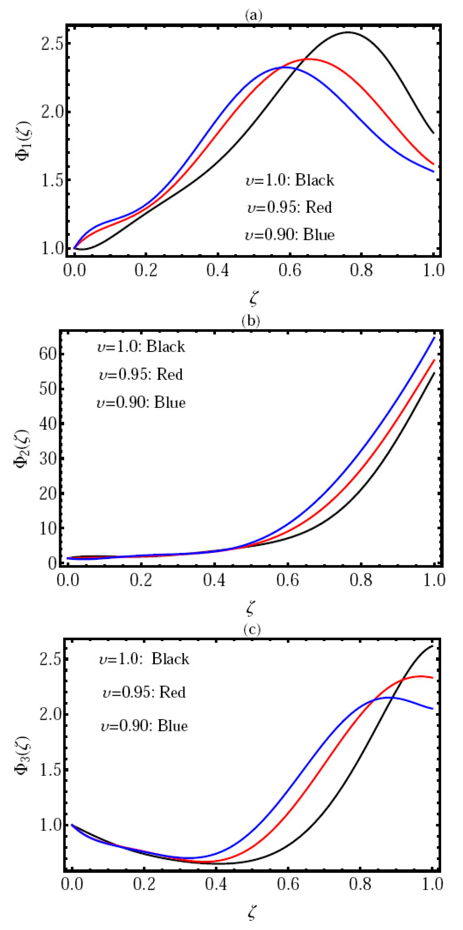
Abstract
:1. Introduction
2. Preliminaries
2.1. Definitions
2.2. Vieta–Lucas Polynomials
3. Numerical Results
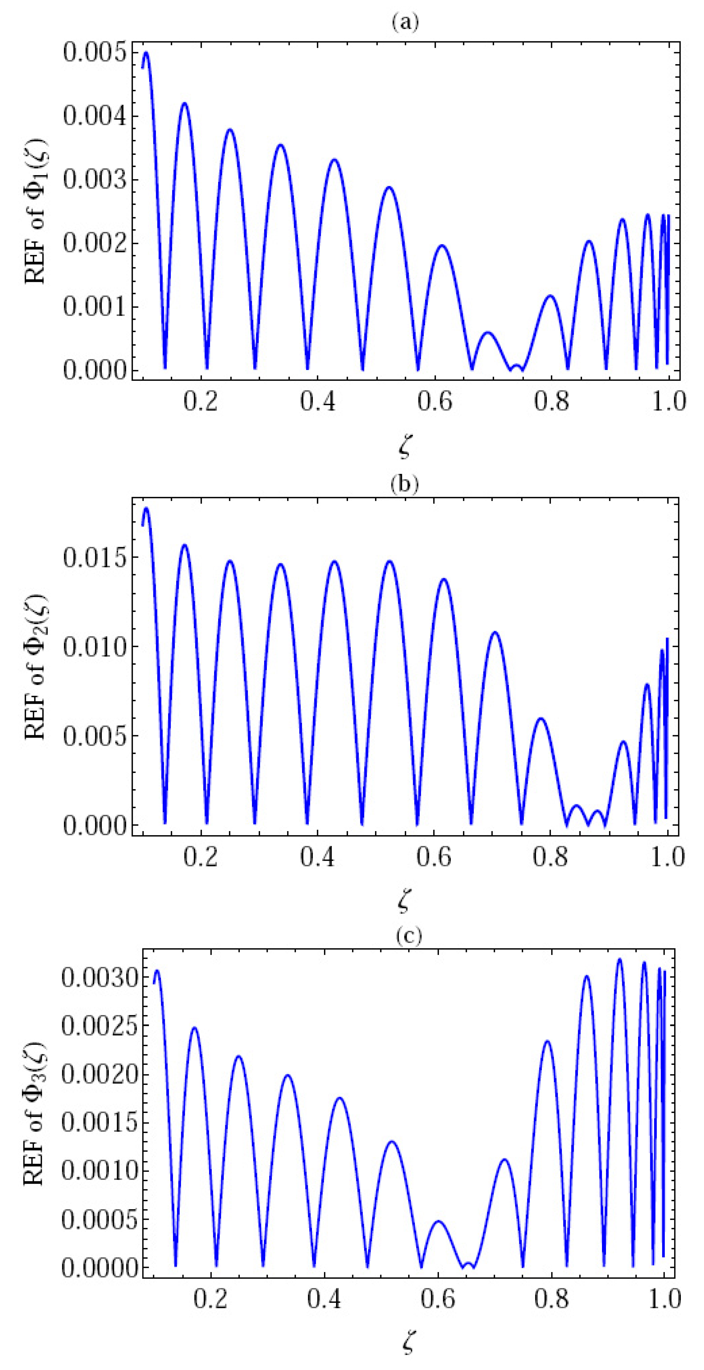
3.1. Convergence Analysis
- The coefficients in the series (10) are bounded, more precisely,
- An error estimate in the -norm is given by
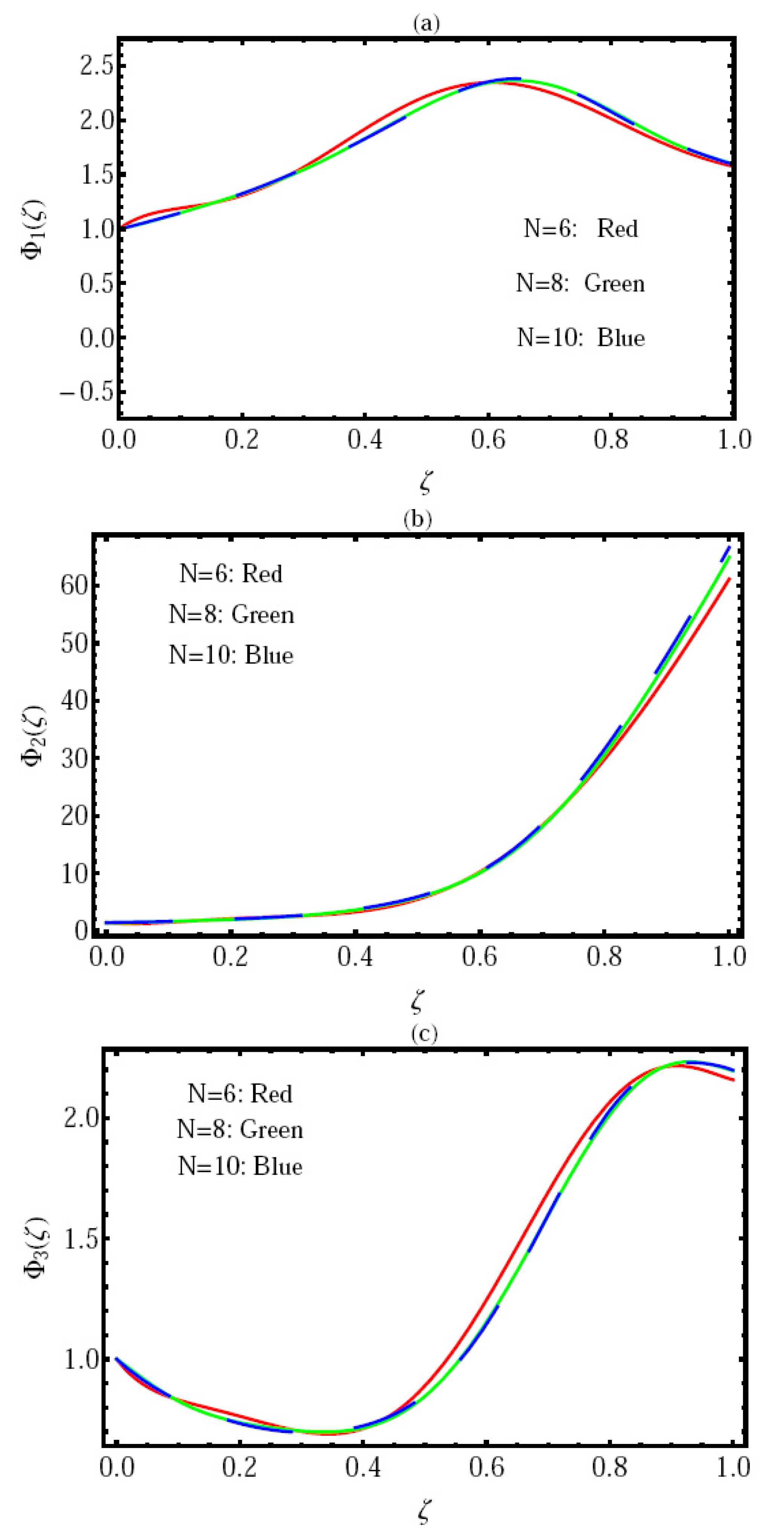
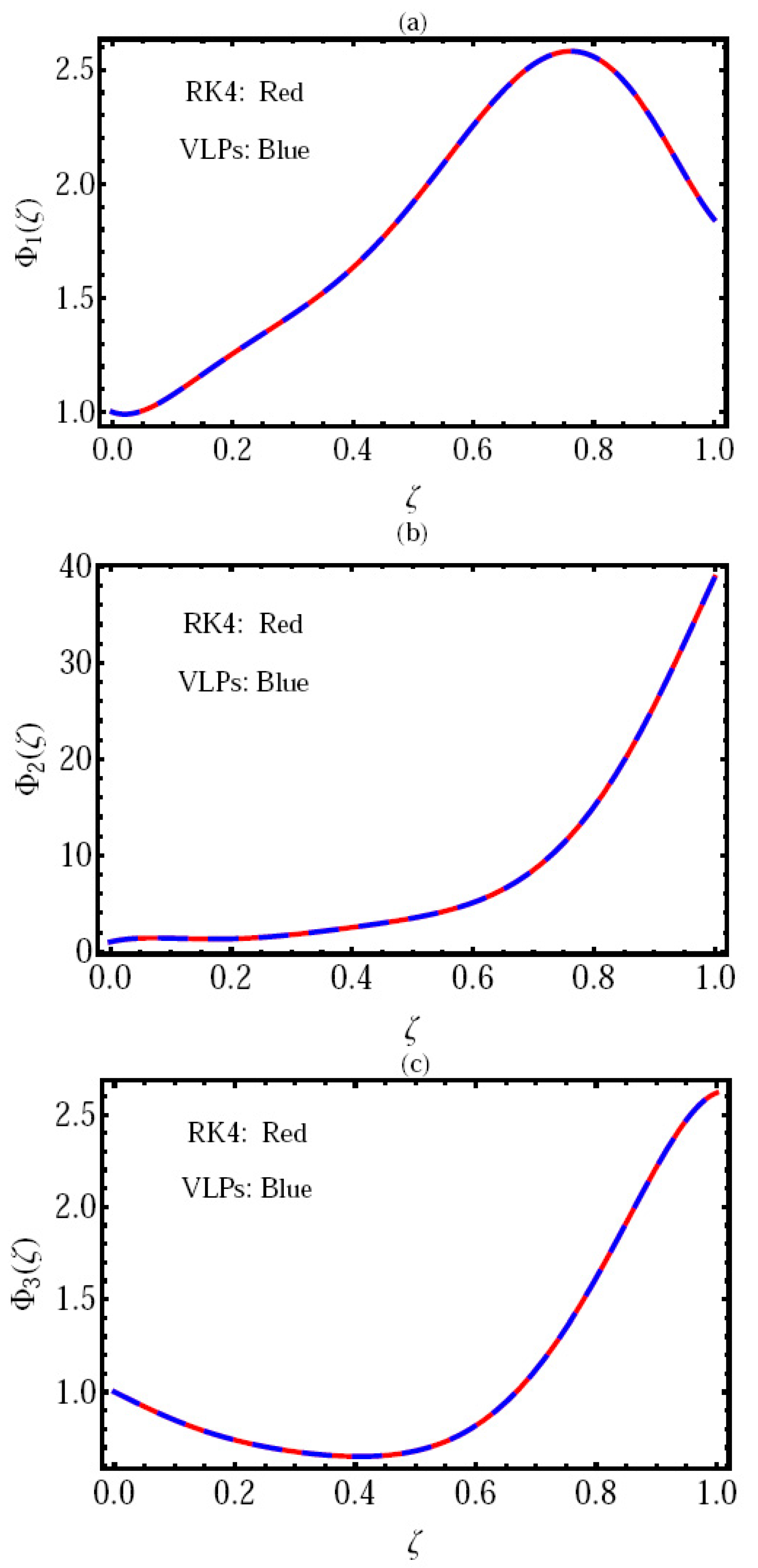
3.2. Computer Simulations
4. Conclusions
- Employing the finite element method for addressing the identical issue: Conducting theoretical investigations into the depth that elucidates the suggested model, incorporating optimal control of the results;
- Adjusting the interpretation of the fractional derivative to alternatives such as the Atangana–Baleanu–Caputo model or a variable-order model.
Author Contributions
Funding
Institutional Review Board Statement
Informed Consent Statement
Data Availability Statement
Conflicts of Interest
References
- Kilbas, S.G.; Kilbas, A.A.; Marichev, O.I. Fractional Integrals and Derivatives: Theory and Applications; Gordon & Breach: Philadelphia, PA, USA, 1993. [Google Scholar]
- Khader, M.M.; Saad, K.M. On the numerical evaluation for studying the fractional KdV, KdV-Burger’s, and Burger’s equations. Eur. Phys. J. Plus 2018, 133, 335. [Google Scholar] [CrossRef]
- Kumar, S.; Nisar, K.S.; Kumar, R.; Cattani, C.; Samet, B. A new Rabotnov fractional-exponential function-based fractional derivative for diffusion equation under external force. Math. Methods Appl. Sci. 2020, 47, 4460–4471. [Google Scholar] [CrossRef]
- Yang, X.J.; Abdel-Aty, M.; Cattani, C. A new general fractional-order derivative with Rabotnov fractional-exponential kernel applied to model the anomalous heat transfer. Therm. Sci. 2019, 23, 1677–1681. [Google Scholar] [CrossRef]
- Gao, W.; Ghanbari, B.; Baskonus, H.M. New numerical simulations for some real-world problems with Atangana-Baleanu fractional derivative. Chaos Solitons Fractals 2019, 128, 34–43. [Google Scholar] [CrossRef]
- Morales-Delgado, V.F.; Gomez-Aguilar, J.F.; Saad, K.M.; Escobar-Jimenez, R.F. Application of the Caputo-Fabrizio and Atangana-Baleanu fractional derivatives to the mathematical model of cancer chemotherapy effect. Math. Methods Appl. Sci. 2019, 42, 1167–1193. [Google Scholar] [CrossRef]
- Toufik, M.; Atangana, A. New numerical approximation of fractional derivative with non-local and non-singular kernel: Application to chaotic models. Eur. Phys. J. Plus 2017, 132, 444. [Google Scholar] [CrossRef]
- Kumar, D.; Singh, J.; Baleanu, D. On the analysis of vibration equation involving a derivative with Mittag-Leffler law. Math. Methods Appl. Sci. 2020, 43, 443–457. [Google Scholar] [CrossRef]
- Abd-Elhameed, W.M.; Youssri, Y.H. Connection formulae between generalized Lucas polynomials and some Jacobi polynomials: Application to certain types of fourth-order BVPs. Int. J. Appl. Comput. Math. 2020, 6, 45. [Google Scholar] [CrossRef]
- Agarwal, F.; El-Sayed, A.A. Vieta–Lucas polynomials for solving a fractional-order mathematical physics model. Adv. Differ. Equ. 2020, 2020, 626. [Google Scholar] [CrossRef]
- Samardzija, N.; Greller, L.D. Explosive route to chaos through a fractal torus in a generalized Lotka–Volterra model. Bull. Math. Biol. 1988, 50, 465–491. [Google Scholar] [CrossRef]
- Diethelm, K. An algorithm for the numerical solution of differential equations of fractional order. Electron. Trans. Numer. Anal. 1997, 5, 1–6. [Google Scholar]
- Khader, M.M.; Babatin, M.M. Numerical treatment for solving fractional SIRC model and influenza A. Comput. Appl. Math. 2014, 33, 543–556. [Google Scholar] [CrossRef]
- Khader, M.M.; Adel, M. Chebyshev wavelet procedure for solving FLDEs. Acta Appl. Math. 2018, 158, 1–10. [Google Scholar] [CrossRef]
- Horadam, A.F. Vieta Polynomials; The University of New England: Armidale, NSW, Australia, 2000. [Google Scholar]
- Zakaria, M.; Khader, M.M.; Al-Dayel, I.; Al-Tayeb, W. Solving fractional generalized Fisher-Kolmogorov-Petrovsky-Piskunov’s equation using compact finite difference method together with spectral collocation algorithms. J. Math. 2022, 2022, 1901131. [Google Scholar]
- Adel, M.; Sweilam, N.H.; Khader, M.M. Semi-analytical scheme with its stability analysis for solving the fractional-order predator–prey equations by using Laplace-VIM. J. Appl. Math. Comput. Mech. 2023, 22, 5–17. [Google Scholar] [CrossRef]
- El-Hawary, H.M.; Salim, M.S.; Hussien, H.S. Ultraspherical integral method for optimal control problems governed by ordinary differential equations. J. Glob. Optim. 2003, 25, 283–303. [Google Scholar] [CrossRef]
- Snyman, J.A. The LFOPC Leap-Frog algorithm for constrained optimization. Comput. Math. Appl. 2000, 40, 1085–1096. [Google Scholar] [CrossRef]
- Zhou, Z.F.; Shi, Y. An ODE method for solving constrained optimization. Comput. Math. Appl. 1997, 3, 97–102. [Google Scholar] [CrossRef]
- Zongfang, Z. A convergence of ODE method in constrained optimization. J. Math. Anal. Appl. 1998, 218, 297–307. [Google Scholar] [CrossRef]
- Parand, K.; Delkhosh, M. Operational matrices to solve nonlinear Volterra-Fredholm integrodifferential equations of multi-arbitrary order. Gazi Univ. J. Sci. 2016, 29, 895–907. [Google Scholar]


Disclaimer/Publisher’s Note: The statements, opinions and data contained in all publications are solely those of the individual author(s) and contributor(s) and not of MDPI and/or the editor(s). MDPI and/or the editor(s) disclaim responsibility for any injury to people or property resulting from any ideas, methods, instructions or products referred to in the content. |
© 2024 by the authors. Licensee MDPI, Basel, Switzerland. This article is an open access article distributed under the terms and conditions of the Creative Commons Attribution (CC BY) license (https://creativecommons.org/licenses/by/4.0/).
Share and Cite
Khader, M.M.; Macías-Díaz, J.E.; Román-Loera, A.; Saad, K.M. A Note on a Fractional Extension of the Lotka–Volterra Model Using the Rabotnov Exponential Kernel. Axioms 2024, 13, 71. https://doi.org/10.3390/axioms13010071
Khader MM, Macías-Díaz JE, Román-Loera A, Saad KM. A Note on a Fractional Extension of the Lotka–Volterra Model Using the Rabotnov Exponential Kernel. Axioms. 2024; 13(1):71. https://doi.org/10.3390/axioms13010071
Chicago/Turabian StyleKhader, Mohamed M., Jorge E. Macías-Díaz, Alejandro Román-Loera, and Khaled M. Saad. 2024. "A Note on a Fractional Extension of the Lotka–Volterra Model Using the Rabotnov Exponential Kernel" Axioms 13, no. 1: 71. https://doi.org/10.3390/axioms13010071