Design of Flotation Circuits Using Tabu-Search Algorithms: Multispecies, Equipment Design, and Profitability Parameters


Abstract
:1. Introduction
2. Background
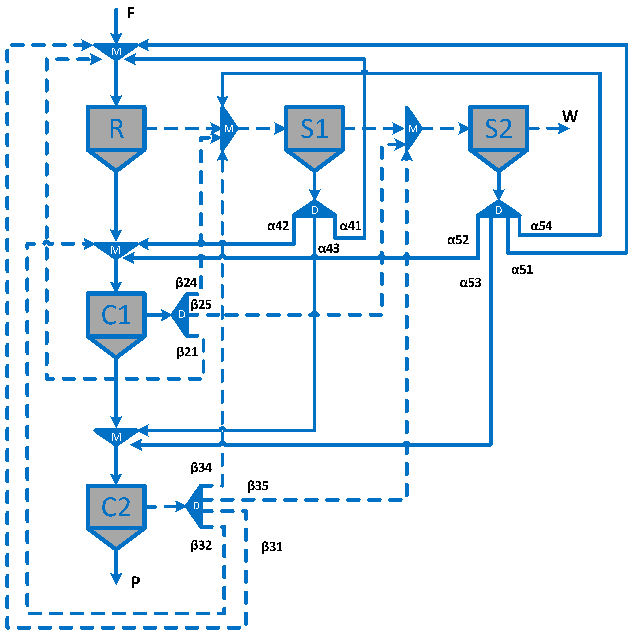
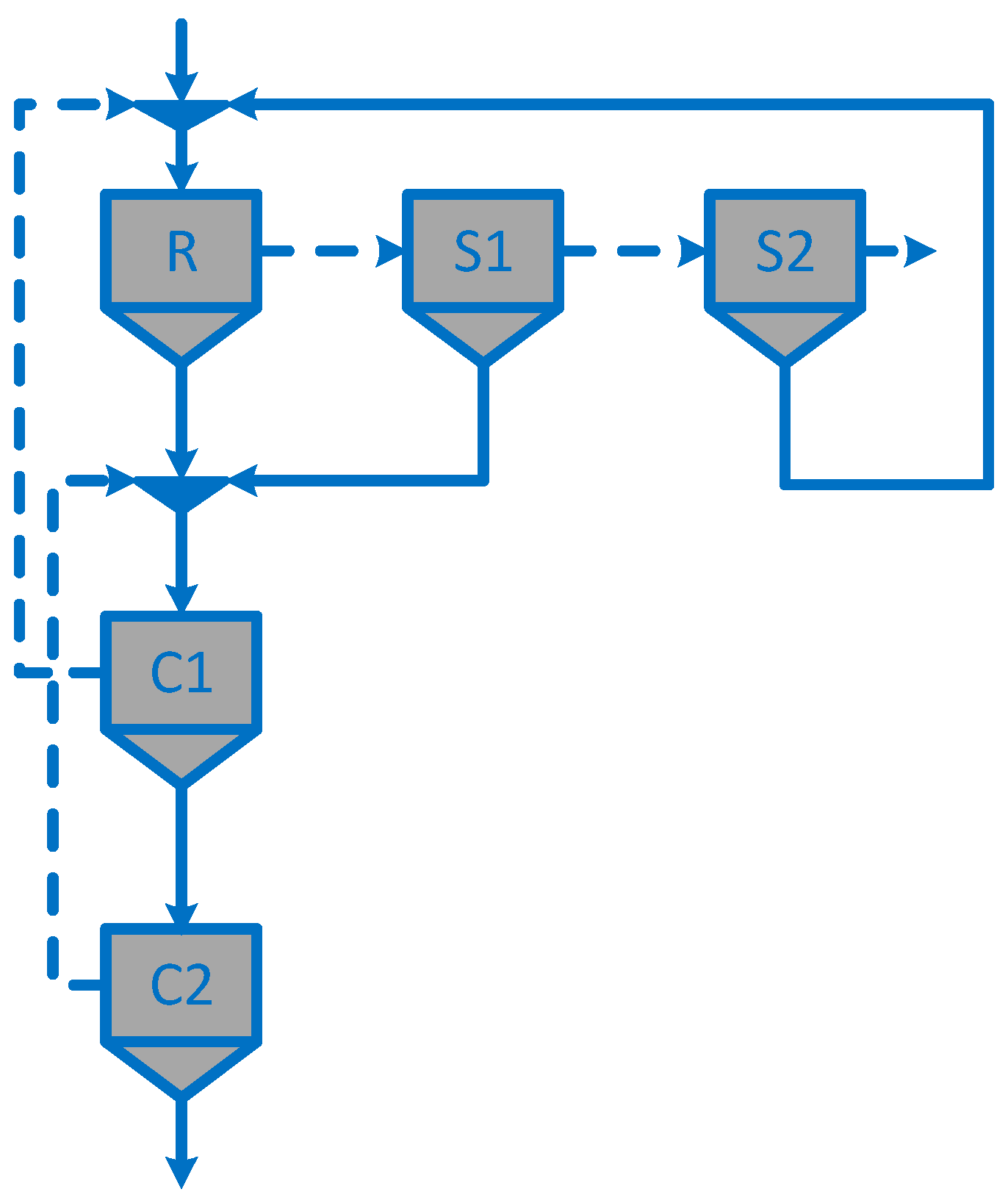
2.1. Superstructure
2.2. Mathematical Model
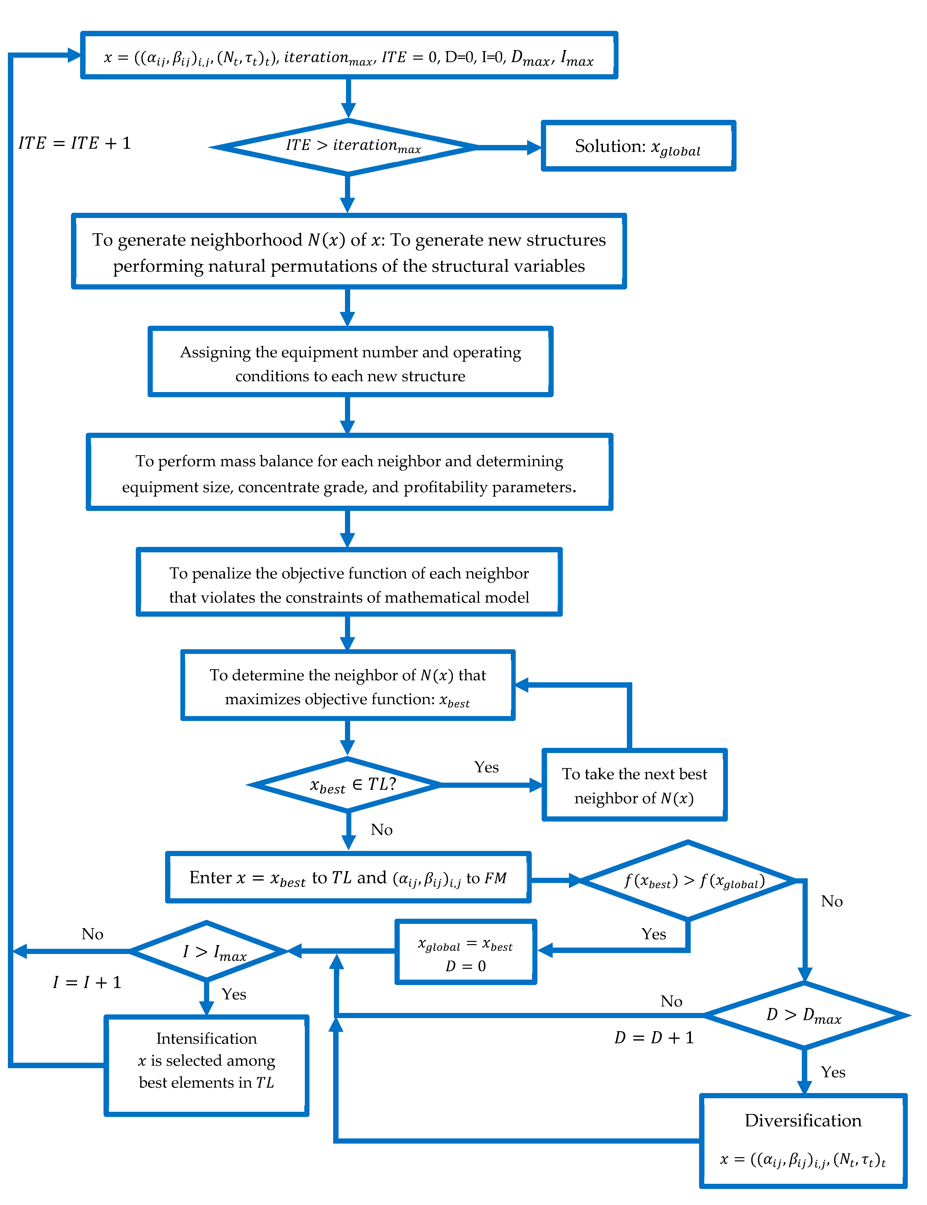
2.3. Optimization Technique: Tabu-Search Algorithm
3. Applications
3.1. Maximization of Revenues
3.2. Maximization of the Net Present Worth
3.3. Benchmarking between the Tabu-Search Algorithm and the Baron Solver
3.4. Comparison with Another Approach
4. Discussion and Conclusions
Author Contributions
Acknowledgments
Conflicts of Interest
Nomenclature
| Cleaner stage | |
| Re-cleaner stage | |
| Concentrate stream of the flotation stage | |
| Mass flow of species in concentrate | |
| Mass flow of species in the concentrate stream from stage to stage | |
| Operating cost of flotation stage | |
| Annual depreciation | |
| Gas factor | |
| Annual cash flows | |
| Lang factor | |
| Lang factor for working capital | |
| Frequency matrix | |
| Grade | |
| Number of hours per year of plant operation | |
| Capital cost | |
| Fixed capital cost | |
| Working capital cost | |
| Mass flow of species in feed streams of stage | |
| Maximum rate constant of the species in flotation stage | |
| Mass flow of species fed to the flotation circuit | |
| Number of flotation cell in stage | |
| Neighborhood of | |
| Life time of the project | |
| Number of rows of Tabu list | |
| Final concentrate | |
| Profits before taxes | |
| Kilowatt-hours cost | |
| Fraction of metal paid | |
| Rougher stage | |
| Recovery of stage for species | |
| Maximum recovery at infinite time of stage for species | |
| Refinery charge | |
| Tax rate | |
| Scavenger stage | |
| Re-scavenger stage | |
| Tail stream of the flotation stage | |
| Mass flow of the species in tail | |
| Mass flow of species in the tail stream from stage to stage | |
| Tabu list | |
| Treatment charge | |
| Cell volumen in stage | |
| Final tail | |
| Net present worth | |
| Best neighbor of | |
| Greek symbols | |
| Decision variables | |
| Decision variables | |
| Penalty parameter | |
| Pulp density | |
| Grade deduction | |
| Cell residence time in stage |
Appendix A
References
- Hu, W.; Hadler, K.; Neethling, S.J.; Cilliers, J.J. Determining flotation circuit layout using genetic algorithms with pulp and froth models. Chem. Eng. Sci. 2013, 102, 32–41. [Google Scholar] [CrossRef]
- Cisternas, L.A.; Lucay, F.A.; Acosta-Flores, R.; Gálvez, E.D. A quasi-review of conceptual flotation design methods based on computational optimization. Miner. Eng. 2018, 117, 24–33. [Google Scholar] [CrossRef]
- Mendez, D.A.; Gálvez, E.D.; Cisternas, L.A. State of the art in the conceptual design of flotation circuits. Int. J. Miner. Process. 2009, 90, 1–15. [Google Scholar] [CrossRef]
- Talbi, E.G. Metaheuristics: From Design to Implementation; John Wiley & Sons: Hoboken, NJ, USA, 2009; ISBN 9780470278581. [Google Scholar]
- Lin, M.H.; Tsai, J.F.; Yu, C.S. A review of deterministic optimization methods in engineering and management. Math. Probl. Eng. 2012, 2012, 756023. [Google Scholar] [CrossRef]
- Glover, F. Future paths for integer programming and links to artificial intelligence. Comput. Oper. Res. 1986, 13, 533–549. [Google Scholar] [CrossRef]
- Osman, I.H.; Laporte, G. Metaheuristics: A bibliography. Ann. Oper. Res. 1996, 63, 511–623. [Google Scholar] [CrossRef]
- Price, K.; Storn, R.M.; Lampinen, J.A. Differential Evolution: A Practical Approach to Global Optimization (Natural Computing Series); Springer: Berlin/Heidelberg, Germany, 2005. [Google Scholar]
- Holland, J.H. Adaptation in Natural and Artificial Systems. MIT Press: Cambridge, MA, USA, 1975. [Google Scholar]
- Moscato, P. On Evolution, Search, Optimization, Genetic Algorithms and Martial Arts: Towards Memetic Algorithms. Caltech Concurrent Computation Program; C3P Report. 1989. Available online: http://citeseer.ist.psu.edu/viewdoc/download?doi=10.1.1.27.9474&rep=rep1&type=pdf (accessed on 31 January 2019).
- Farmer, J.D.; Packard, N.H.; Perelson, A.S. The immune system, adaptation, and machine learning. Phys. D Nonlinear Phenom. 1986, 22, 187–204. [Google Scholar] [CrossRef]
- Kirkpatrick, S.; Gelatt, C.D.; Vecchi, M.P. Optimization by simulated annealing. Science 1983, 220, 671–680. [Google Scholar] [CrossRef] [PubMed]
- Dorigo, M. Optimization, Learning and Natural Algorithms. Ph.D. Thesis, Dipartimento di Elettronica, Politecnico di Milano, Milan, Italy, 1992. [Google Scholar] [CrossRef]
- Kennedy, J.; Eberhart, R. Particle Swarm Optimization. In Proceedings of the IEEE International Conference on Neural Networks, Perth, WA, Australia, 27 November–1 December 1995; Volume IV, pp. 1942–1948. [Google Scholar]
- Glover, F.; Laguna, M. Tabu Search. In Handbook of Combinatorial Optimization; Du, D.Z., Pardalos, P.M., Eds.; Springer: Boston, MA, USA, 1998; pp. 2093–2229. ISBN 978-1-4613-0303-9. [Google Scholar]
- Glover, F. Tabu Search-Part I. ORSA J. Comput. 1989, 1, 190–206. [Google Scholar] [CrossRef]
- Han, S.; Li, J.; Liu, Y. Tabu search algorithm optimized ANN model for wind power prediction with NWP. Energy Procedia 2011, 12, 733–740. [Google Scholar] [CrossRef]
- Ting, C.K.; Li, S.T.; Lee, C. On the harmonious mating strategy through tabu search. Inf. Sci. 2003, 156, 189–214. [Google Scholar] [CrossRef]
- Soto, M.; Sevaux, M.; Rossi, A.; Reinholz, A. Multiple neighborhood search, tabu search and ejection chains for the multi-depot open vehicle routing problem. Comput. Ind. Eng. 2017, 107, 211–222. [Google Scholar] [CrossRef]
- Lin, B.; Miller, D.C. Application of tabu search to model indentification. In Proceedings of the AIChE Annual Meeting, Los Angeles, CA, USA, 12–17 November 2000. [Google Scholar]
- Kulturel-Konak, S.; Smith, A.E.; Coit, D.W. Efficiently solving the redundancy allocation problem using tabu search. IIE Trans. (Inst. Ind. Eng.) 2003, 35, 515–526. [Google Scholar] [CrossRef]
- Kis, T. Job-shop scheduling with processing alternatives. Eur. J. Oper. Res. 2003, 151, 307–332. [Google Scholar] [CrossRef]
- Pan, Q.K.; Fatih Tasgetiren, M.; Liang, Y.C. A discrete particle swarm optimization algorithm for the no-wait flowshop scheduling problem. Comput. Oper. Res. 2008, 35, 2807–2839. [Google Scholar] [CrossRef]
- Mandani, F.; Camarda, K. Multi-objective Optimization for Plant Design via Tabu Search. Comput. Aided Chem. Eng. 2018, 43, 543–548. [Google Scholar]
- Mehrotra, S.P.; Kapur, P.C. Optimal-Suboptimal Synthesis and Design of Flotation Circuits. Sep. Sci. 1974, 9, 167–184. [Google Scholar] [CrossRef]
- Reuter, M.A.; van Deventer, J.S.J.; Green, J.C.A.; Sinclair, M. Optimal design of mineral separation circuits by use of linear programming. Chem. Eng. Sci. 1988, 43, 1039–1049. [Google Scholar] [CrossRef]
- Reuter, M.A.; Van Deventer, J.S.J. The use of linear programming in the optimal design of flotation circuits incorporating regrind mills. Int. J. Miner. Process. 1990, 28, 15–43. [Google Scholar] [CrossRef]
- Schena, G.; Villeneuve, J.; Noël, Y. A method for a financially efficient design of cell-based flotation circuits. Int. J. Miner. Process. 1996, 46, 1–20. [Google Scholar] [CrossRef]
- Schena, G.D.; Zanin, M.; Chiarandini, A. Procedures for the automatic design of flotation networks. Int. J. Miner. Process. 1997, 52, 137–160. [Google Scholar] [CrossRef]
- Maldonado, M.; Araya, R.; Finch, J. Optimizing flotation bank performance by recovery profiling. Miner. Eng. 2011, 24, 939–943. [Google Scholar] [CrossRef]
- Cisternas, L.A.; Méndez, D.A.; Gálvez, E.D.; Jorquera, R.E. A MILP model for design of flotation circuits with bank/column and regrind/no regrind selection. Int. J. Miner. Process. 2006, 79, 253–263. [Google Scholar] [CrossRef]
- Cisternas, L.A.; Gálvez, E.D.; Zavala, M.F.; Magna, J. A MILP model for the design of mineral flotation circuits. Int. J. Miner. Process. 2004, 74, 121–131. [Google Scholar] [CrossRef]
- Calisaya, D.A.; López-Valdivieso, A.; de la Cruz, M.H.; Gálvez, E.E.; Cisternas, L.A. A strategy for the identification of optimal flotation circuits. Miner. Eng. 2016, 96–97, 157–167. [Google Scholar] [CrossRef]
- Acosta-Flores, R.; Lucay, F.A.; Cisternas, L.A.; Galvez, E.D. Two-phase optimization methodology for the design of mineral flotation plants, including multispecies and bank or cell models. Miner. Metall. Process. 2018, 35, 24–34. [Google Scholar] [CrossRef]
- Guria, C.; Verma, M.; Mehrotra, S.P.; Gupta, S.K. Multi-objective optimal synthesis and design of froth flotation circuits for mineral processing, using the jumping gene adaptation of genetic algorithm. Ind. Eng. Chem. Res. 2005, 44, 2621–2633. [Google Scholar] [CrossRef]
- Guria, C.; Verma, M.; Gupta, S.K.; Mehrotra, S.P. Simultaneous optimization of the performance of flotation circuits and their simplification using the jumping gene adaptations of genetic algorithm. Int. J. Miner. Process. 2005, 77, 165–185. [Google Scholar] [CrossRef]
- Ghobadi, P.; Yahyaei, M.; Banisi, S. Optimization of the performance of flotation circuits using a genetic algorithm oriented by process-based rules. Int. J. Miner. Process. 2011, 98, 174–181. [Google Scholar] [CrossRef]
- Pirouzan, D.; Yahyaei, M.; Banisi, S. Pareto based optimization of flotation cells configuration using an oriented genetic algorithm. Int. J. Miner. Process. 2014, 126, 107–116. [Google Scholar] [CrossRef]
- Cisternas, L.A.; Jamett, N.; Gálvez, E.D. Approximate recovery values for each stage are sufficient to select the concentration circuit structures. Miner. Eng. 2015, 83, 175–184. [Google Scholar] [CrossRef]
- Sepúlveda, F.D.; Lucay, F.; González, J.F.; Cisternas, L.A.; Gálvez, E.D. A methodology for the conceptual design of flotation circuits by combining group contribution, local/global sensitivity analysis, and reverse simulation. Int. J. Miner. Process. 2017, 164, 56–66. [Google Scholar] [CrossRef]
- Yianatos, J.B.; Henríquez, F.D. Short-cut method for flotation rates modelling of industrial flotation banks. Miner. Eng. 2006, 19, 1336–1340. [Google Scholar] [CrossRef]
- Green, J.C.A. The optimisation of flotation networks. Int. J. Miner. Process. 1984, 13, 83–103. [Google Scholar] [CrossRef]
- Cisternas, L.A.; Lucay, F.; Gálvez, E.D. Effect of the objective function in the design of concentration plants. Miner. Eng. 2014, 63, 16–24. [Google Scholar] [CrossRef]
- Ruhmer, W. Handbook on the Estimation of Metallurgical Process Cost, 2nd ed.; Mintek: Randburg, South Africa, 1991. [Google Scholar]
- Peters, M.S.; Timmerhaus, K.D.; West, R.E. Plant Design and Economics for Chemical Engineers, 4th ed.; McGraw-Hill Publishing Company: New York, NY, USA, 1991; ISBN 0070496137. [Google Scholar]
- Masuda, K.; Kurihara, K.; Aiyoshi, E. A penalty approach to handle inequality constraints in particle swarm optimization. In Proceedings of the IEEE International Conference on Systems, Man and Cybernetics, Istanbul, Turkey, 10–13 October 2010. [Google Scholar]
- Gogna, A.; Tayal, A. Metaheuristics: Review and application. J. Exp. Theor. Artif. Intell. 2013, 25, 503–526. [Google Scholar] [CrossRef]
- Gendreau, M.; Potvin, J.-Y. Variable Nneighborhood search (chapter). In Handbook of Metaheuristics; Springer: Berlin, Germany, 2010. [Google Scholar] [CrossRef]
- López, E.; Salas, Ó.; Murillo, Á. A deterministic algorithm using tabu search. Revista de Matemática Teoría y Aplicaciones 2014, 21, 127–144. [Google Scholar] [CrossRef]
- De los cobos, S.G.; Goddard, J.; Gutiérrez, M.; Martínez, A. Búsqueda y Exploración Estocástica, 1st ed.; Universidad Autonoma Metropolitana: Mexico City, Mexico, 2010; ISBN 9786074772395. [Google Scholar]
- Jamett, N.; Cisternas, L.A.; Vielma, J.P. Solution strategies to the stochastic design of mineral flotation plants. Chem. Eng. Sci. 2015, 134, 850–860. [Google Scholar] [CrossRef] [Green Version]
- Lin, B.; Chavali, S.; Camarda, K.; Miller, D.C. Using Tabu search to solve MINLP problems for PSE. Comput. Aided Chem. Eng. 2003, 15, 541–546. [Google Scholar] [CrossRef]
- Fouskakis, D.; Draper, D. Stochastic optimization: A review. Int. Stat. Rev. 2002, 70, 315–349. [Google Scholar] [CrossRef]


| Species | Copper Grade wt % | Feed (t/h) |
|---|---|---|
| Chalcopyrite fast (Cpf) | 0.35 | 15 |
| Chalcopyrite slow (Cpy) | 0.25 | 8 |
| Chalcocite fast (Cf) | 0.1 | 5 |
| Chalcocite slow (Cs) | 0.07 | 3 |
| Pyrite (P) | 0.0 | 4 |
| Silica (S) | 0.0 | 200 |
| Gangue (G) | 0.0 | 300 |
| Stage\Species | Cpf | Cpy | Cf | Cs | P | S | G | Cpg | Cpy | Cf | Cs | P | S | F |
|---|---|---|---|---|---|---|---|---|---|---|---|---|---|---|
| R | 1.85 | 1.50 | 1.00 | 0.70 | 0.80 | 0.60 | 0.30 | 0.90 | 0.85 | 0.85 | 0.75 | 0.80 | 0.60 | 0.20 |
| C1 | 1.30 | 1.00 | 0.80 | 0.40 | 0.70 | 0.30 | 0.20 | 0.75 | 0.70 | 0.70 | 0.60 | 0.60 | 0.50 | 0.15 |
| C2 | 1.30 | 1.00 | 0.80 | 0.40 | 0.70 | 0.30 | 0.20 | 0.70 | 0.65 | 0.65 | 0.50 | 0.60 | 0.50 | 0.15 |
| S1 | 1.85 | 1.50 | 1.00 | 0.70 | 0.80 | 0.60 | 0.30 | 0.90 | 0.85 | 0.85 | 0.75 | 0.80 | 0.60 | 0.20 |
| S2 | 1.85 | 1.50 | 1.00 | 0.70 | 0.80 | 0.60 | 0.30 | 0.90 | 0.85 | 0.85 | 0.75 | 0.80 | 0.60 | 0.20 |
| Case | 1 | 2 | 3 | 4 | 5 | |||||
|---|---|---|---|---|---|---|---|---|---|---|
| Algorithm | Tabu | Baron | Tabu | Baron | Tabu | Baron | Tabu | Baron | Tabu search | Baron |
| Species | Cpf, Cps, S, G | Cpf, Cps, P, S, G | Cpf, Cps, Cf, P, S, G | Cpf, Cps, Cf, Cs, P, S, G | Cpf, Cps, Cf, Cs, Bof, P, S, G | |||||
| Revenue, USD/year | 132,318,860 | 132,323,459 | 132,852,410 | 132,854,057 | 130,981,546 | 130,981,549 | 130,960,079 | 130,958,748 | 129,185,242 | 130,335,529 |
| Net present worth, USD | 612,961,580 | 612,702,132 | 618,316,980 | 617,392,845 | 598,070,573 | 598,081,544 | 595,475,455 | 599,377,620 | 671,113,149 | 692,374,613 |
| Profit before taxes, USD/year | 94,235,451 | 94,208,659 | 94,972,404 | 94,849,038 | 92,078,958 | 92,080,433 | 91,716,855 | 92,213,521 | 101,068,398 | 103,931,519 |
| Total capital investment, USD | 52,137,292 | 52,317,036 | 51,261,610 | 51,471,333 | 52,917,663 | 52,915,338 | 53,265,087 | 52,005,813 | 24,608,590 | 20,166,465 |
| Total annual cost, USD/year | 35,259,307 | 35,280,960 | 35,103,337 | 35,216,989 | 36,036,215 | 36,034,869 | 36,358,032 | 35,928,246 | 26,783,878 | 25,311,660 |
| , | 182.822 | 182.54 | 181.825 | 185.596 | 195.500 | 195.46 | 197.704 | 197.60 | 119.350 | 111.037 |
| , | 21.222 | 20.31 | 22.805 | 22.872 | 22.442 | 22.44 | 22.712 | 22.63 | 25.841 | 20.083 |
| , | 7.761 | 7.15 | 8.973 | 8.800 | 9.964 | 9.96 | 9.984 | 9.98 | 14.138 | 10.287 |
| , | 163.211 | 163.17 | 163.697 | 163.700 | 165.782 | 165.78 | 167.565 | 167.59 | 159.679 | 101.602 |
| , | 153.893 | 153.88 | 153.971 | 153.972 | 154.464 | 154.46 | 155.908 | 155.91 | 151.817 | 155.590 |
| , min | 5.000 | 5.000 | 4.900 | 5.000 | 5.000 | 5.000 | 5.000 | 5.000 | 3.300 | 3.000 |
| , min | 3.130 | 3.000 | 3.000 | 3.000 | 3.000 | 3.000 | 3.000 | 3.000 | 4.300 | 3.000 |
| , min | 3.320 | 3.000 | 3.070 | 3.000 | 3.000 | 3.000 | 3.000 | 3.000 | 4.400 | 3.000 |
| , min | 5.000 | 5.000 | 5.000 | 5.000 | 5.000 | 5.000 | 5.000 | 5.000 | 4.400 | 3.000 |
| , min | 5.000 | 5.000 | 5.000 | 5.000 | 5.000 | 5.000 | 5.000 | 5.000 | 4.800 | 4.920 |
| 15.000 | 15.000 | 14.000 | 14.000 | 15.000 | 15.000 | 15.000 | 14.000 | 3.000 | 3.000 | |
| 4.000 | 5.000 | 5.000 | 5.000 | 3.000 | 3.000 | 3.000 | 3.000 | 3.000 | 3.000 | |
| 3.000 | 3.000 | 3.000 | 3.000 | 3.000 | 3.000 | 3.000 | 3.000 | 3.000 | 3.000 | |
| 15.000 | 15.000 | 15.000 | 15.000 | 15.000 | 15.000 | 15.000 | 15.000 | 9.000 | 3.000 | |
| 15.000 | 15.000 | 15.000 | 15.000 | 15.000 | 15.000 | 15.000 | 15.000 | 10.000 | 13.000 | |
| Grade Cu | 0.3123 | 0.312 | 0.274 | 0.274 | 0.257 | 0.257 | 0.257 | 0.257 | 0.250 | 0.250 |
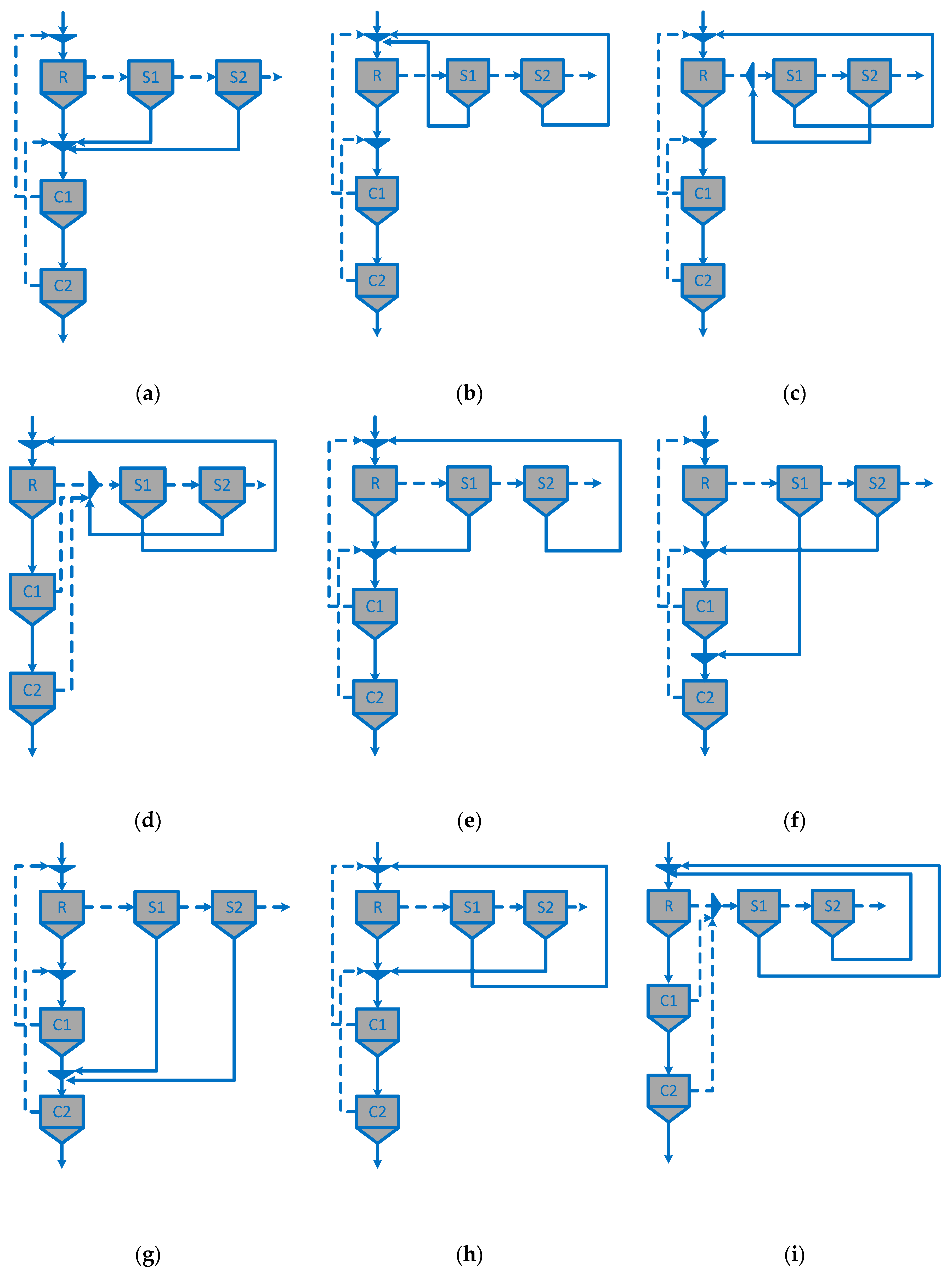
| Circuit structure | Figure 4 | Figure 4 | Figure 4 | Figure 4 | Figure 3 | Figure 3 | Figure 3 | Figure 3 | Figure 5d | Figure 5c |
| Time, s | 46.610 | 233.000 | 176.580 | 423.030 | 287.670 | 9026.190 | 601.630 | 14,640.00 | 433.930 | 10,257.020 |
| Iterations of algorithm | 1000 | - | 1000 | - | 1500 | - | 2000 | - | 3000 | - |
| Neighborhood size | 40 | - | 130 | - | 150 | - | 170 | - | 60 | - |
| Iterations of diversification | 50 | - | 20 | - | 30 | - | 30 | - | 20 | - |
| Iteration of intensification | 10 | - | 40 | - | 40 | - | 50 | - | 50 | - |
| No. rows of Tabu list | 100 | - | 50 | - | 50 | - | 50 | - | 50 | - |
| Case | 1 | 2 | 3 | 4 | 5 | 6 | ||||||
|---|---|---|---|---|---|---|---|---|---|---|---|---|
| Algorithm | Tabu | Baron | Tabu | Baron | Tabu | Baron | Tabu | Baron | Tabu | Baron | Tabu | Baron |
| Species | Cpf, Cps, S, G | Cpf, Cps, P, S, G | Cpf, Cps, Cf, P, S, G | Cpf, Cps, Cf, Cs, P, S, G | Cpf, Cps, Cf, Cs, Bof, P, S, G | Cpf, Cps, Cf, Cs, Bof, Bos, P, S, G | ||||||
| Net present worth, USD | 735,935,440 | 735,938,754 | 737,697,720 | 737,697,912 | 726,139,400 | 726,139,411 | 724,828,320 | 724,828,404 | 723,842,180 | 723,842,865 | 719,710,450 | 719,712,493 |
| Revenue, USD/year | 130,918,800 | 130,920,451 | 131,435,920 | 131,433,456 | 129,853,889 | 129,853,889 | 129,830,340 | 129,830,357 | 129,839,150 | 129,840,240 | 129,548,420 | 129,551,233 |
| Profit before taxes, USD/year | 109,609,160 | 109,606,145 | 109,882,230 | 109,881,842 | 108,168,025 | 108,168,032 | 107,977,400 | 107,977,414 | 107,833,120 | 107,833,404 | 107,267,450 | 107,268,177 |
| Total capital inv., USD | 8,162,377 | 8,108,261 | 8,345,130 | 8,338,775 | 8,329,184 | 8,329,184 | 8,386,189 | 8,386,191 | 8,415,244 | 8,418,023 | 9,135,362 | 9,141,936 |
| Total annual cost, USD/year | 20,867,504 | 20,875,109 | 21,101,667 | 21,099,930 | 21,234,694 | 21,234,694 | 21,398,690 | 21,398,690 | 21,550,197 | 21,550,859 | 21,786,145 | 21,787,868 |
| , | 101.244 | 101.240 | 103.058 | 103.070 | 105.819 | 105.820 | 106.847 | 106.850 | 111.845 | 111.807 | 111.390 | 111.325 |
| , | 15.985 | 17.190 | 18.905 | 18.700 | 19.595 | 19.600 | 19.847 | 19.840 | 25.510 | 25.520 | 21.292 | 21.620 |
| , | 6.619 | 8.390 | 8.112 | 8.110 | 9.578 | 9.580 | 9.600 | 9.600 | 10.266 | 10.412 | 10.252 | 10.260 |
| , | 93.280 | 93.280 | 93.795 | 93.800 | 94.817 | 94.820 | 95.722 | 95.720 | 97.236 | 97.225 | 99.287 | 99.265 |
| , | 90.073 | 90.070 | 90.219 | 90.220 | 90.615 | 90.620 | 91.412 | 91.410 | 91.901 | 91.898 | 92.295 | 92.322 |
| , min | 3.000 | 3.000 | 3.000 | 3.000 | 3.000 | 3.000 | 3.000 | 3.000 | 3.000 | 3.000 | 3.000 | 3.000 |
| , min | 3.000 | 3.200 | 3.080 | 3.040 | 3.000 | 3.000 | 3.000 | 3.000 | 3.960 | 3.973 | 3.200 | 3.256 |
| , min | 3.000 | 3.730 | 3.000 | 3.000 | 3.000 | 3.000 | 3.000 | 3.000 | 3.000 | 3.051 | 3.000 | 3.000 |
| , min | 3.000 | 3.000 | 3.000 | 3.000 | 3.000 | 3.000 | 3.000 | 3.000 | 3.000 | 3.000 | 3.000 | 3.000 |
| , min | 3.000 | 3.000 | 3.000 | 3.000 | 3.000 | 3.000 | 3.000 | 3.000 | 3.000 | 3.000 | 3.000 | 3.001 |
| 3.000 | 3.000 | 3.000 | 3.000 | 3.000 | 3.000 | 3.000 | 3.000 | 3.000 | 3.000 | 3.000 | 3.000 | |
| 4.000 | 4.000 | 4.000 | 4.000 | 4.000 | 4.000 | 4.000 | 4.000 | 3.000 | 3.000 | 3.000 | 3.000 | |
| 4.000 | 3.000 | 4.000 | 4.000 | 3.000 | 3.000 | 3.000 | 3.000 | 3.000 | 3.000 | 3.000 | 3.000 | |
| 3.000 | 3.000 | 3.000 | 3.000 | 3.000 | 3.000 | 3.000 | 3.000 | 3.000 | 3.000 | 4.000 | 4.000 | |
| 3.000 | 3.000 | 3.000 | 3.000 | 3.000 | 3.000 | 3.000 | 3.000 | 3.000 | 3.000 | 3.000 | 3.000 | |
| Grade Cu | 0.3125 | 0.3130 | 0.276 | 0.276 | 0.2608 | 0.261 | 0.2607 | 0.261 | 0.250 | 0.250 | 0.250 | 0.250 |
| Circuit structure | Figure 5a | Figure 5a | Figure 5a | Figure 5a | Figure 4 | Figure 4 | Figure 4 | Figure 4 | Figure 3 | Figure 3 | Figure 5c | Figure 5c |
| Time, s | 106.260 | 94.200 | 424.720 | 294.920 | 464.990 | 533.400 | 527.610 | 355.200 | 710.040 | 1082.640 | 875.980 | 4299.860 |
| No. rows Tabu list | 50 | - | 50 | - | 50 | - | 50 | - | 50 | - | 50 | - |
| No. iterations of algorithm | 2000 | - | 2000 | - | 2000 | - | 2000 | - | 2000 | - | 2000 | - |
| Iteration of diversification | 30 | - | 30 | - | 30 | - | 30 | - | 30 | - | 30 | - |
| Iteration of intensification | 50 | - | 40 | - | 40 | - | 50 | - | 50 | - | 50 | - |
| Neighborhood size | 70 | - | 130 | - | 150 | - | 170 | - | 190 | - | 210 | - |
| Case | 1 | 2 | 3 | 4 | 5 | 6 | ||||||
|---|---|---|---|---|---|---|---|---|---|---|---|---|
| Algorithm | Tabu | Baron | Tabu | Baron | Tabu | Baron | Tabu | Baron | Tabu | Baron | Tabu | Baron |
| Species | Cpf, S, G | Cpf, Cps, S, G | Cpf, Cps, Pf, S, G | Cpf, Cps, Pf, Ps, S, G | Cpf, Cps, Cf, Pf, Ps, S, G | Cpf, Cps, Cf, Cs, Pf, Ps, S, G | ||||||
| Revenue, USD/year | 26,455,569 | 26,455,571 | 38,755,316 | did not converge after 5 days | 38,568,418 | did not converge after 5 days | 38,567,734 | did not converge after 5 days | 36,714,037 | did not converge after 5 days | There is no solution | There is no solution |
| , min | 5.000 | 5.000 | 5.000 | - | 5.000 | - | 5000 | - | 3.260 | - | - | - |
| , min | 3.000 | 3.000 | 3.090 | - | 3.000 | - | 3000 | - | 3.000 | - | - | - |
| , min | 3.000 | 3.000 | 3.000 | - | 3.000 | - | 3000 | - | 3.000 | - | - | - |
| , min | 5.000 | 5.000 | 5.000 | - | 5.000 | - | 5000 | - | 5.000 | - | - | - |
| , min | 5.000 | 5.000 | 5.000 | - | 5.000 | - | 5000 | - | 3.800 | - | - | - |
| 15.000 | 15.000 | 15.000 | - | 15.000 | - | 15,000 | - | 5.000 | - | - | - | |
| 5.000 | 5.000 | 3.000 | - | 4.000 | - | 4000 | - | 3.000 | - | - | - | |
| 3.000 | 3.000 | 3.000 | - | 3.000 | - | 3000 | - | 3.000 | - | - | - | |
| 15.000 | 15.000 | 15.000 | - | 15.000 | - | 15,000 | - | 6.000 | - | - | - | |
| 15.000 | 15.000 | 15.000 | - | 15.000 | - | 15,000 | - | 6.000 | - | - | - | |
| Grade Cu | 0.345 | 0.345 | 0.304 | - | 0.303 | - | 0.303 | - | 0.250 | - | - | - |
| Circuit structure | Figure 3 | Figure 3 | Figure 3 | - | Figure 4 | - | Figure 4 | - | Figure 5i | - | - | - |
| Time, s | 54.900 | 1961.830 | 120.040 | - | 165.340 | - | 216.390 | - | 472.720 | - | - | - |
| No. rows Tabu list | 100 | - | 50 | - | 50 | - | 100 | - | 50 | - | - | - |
| No. iterations of algorithm | 1000 | - | 1000 | - | 1000 | - | 1000 | - | 1000 | - | - | - |
| Iteration of diversification | 30 | - | 20 | - | 20 | - | 20 | - | 20 | - | - | - |
| Iteration of intensification | 100 | - | 40 | - | 40 | - | 40 | - | 40 | - | - | - |
| Neighborhood size | 90 | - | 110 | - | 130 | - | 150 | - | 170 | - | - | - |
| Algorithm | Tabu Search | Baron | |||
|---|---|---|---|---|---|
| Revenue, USD $1000/year | 49,792 | 49,306 | 49,783 | 49,543 | 49,792 |
| , min | 6.000 | 6.000 | 6.000 | 6.000 | 6.000 |
| , min | 3.020 | 6.000 | 2.349 | 6.000 | 2.978 |
| , min | 0.500 | 0.500 | 0.500 | 0.500 | 0.500 |
| , min | 6.000 | 2.424 | 6.000 | 1.816 | 6.000 |
| , min | 6.000 | 2.424 | 6.000 | 6.000 | 6.000 |
| 15.000 | 15.000 | 15.000 | 15,000 | 15.000 | |
| 8.000 | 8.000 | 8.000 | 8.000 | 8.000 | |
| 5.000 | 2.000 | 6.000 | 2.000 | 5.000 | |
| 15.000 | 15.000 | 15.000 | 15.000 | 15.000 | |
| 15.000 | 15.000 | 15.000 | 10.000 | 15.000 | |
| Grade Cu | 0.222 | 0.220 | 0.222 | 0.222 | 0.222 |
| Circuit structure | Figure 4 | Figure 5g (circuit 1) * | Figure 5a (circuit 2) * | Figure 5f (circuit 3) * | Figure 4 (circuit 4) * |
| Time, s | 798.06 | 605,789.65 | 628,906.07 | 630,906.7 | 80,193.67 |
| Algorithm | Best Design | Secondary Designs | ||
|---|---|---|---|---|
| Revenue, USD/year | 49,792,2192 | 49,698,998 | 49,670,988 | 49,575,119 |
| , min | 6.000 | 4.190 | 4.780 | 3.200 |
| , min | 3.020 | 5.160 | 5.680 | 5.700 |
| , min | 0.500 | 5.390 | 4.260 | 6.000 |
| , min | 6.000 | 5.850 | 5.640 | 5.950 |
| , min | 6.000 | 6.000 | 5.200 | 5.210 |
| 15.000 | 15.000 | 15.000 | 9.000 | |
| 8.000 | 4.000 | 3.000 | 2.000 | |
| 5.000 | 2.000 | 2.000 | 3.000 | |
| 15.000 | 15.000 | 15.000 | 7.000 | |
| 15.000 | 15.000 | 15.000 | 11.000 | |
| Grade Cu | 0.222 | 0.222 | 0.222 | 0.222 |
| Circuit structure | Figure 4 | Figure 5b | Figure 5h | Figure 5e |
| Algorithm | Tabu Search | Baron Solver |
|---|---|---|
| Advantages | The convergence is fast. The algorithm always provides a solution when the mathematical model is well defined. The algorithm is flexible, i.e., it allows the use of other methods, such as linear programming algorithms. The algorithm provides good quality solutions. The algorithm provides secondary designs. | The solver provides a global optimal design when converged. The solver does not need to adjust parameters for providing a solution. The obtained designs do not change if the solver is run again. |
| Disadvantages | Some algorithm parameters, such as neighborhood size and number of iterations of the algorithm, among others, must be adjusted for finding a good quality solution. Penalty parameters must be used for satisfying the constraints of the mathematical model. The obtained designs could change if the algorithm is run again. The algorithm must incorporate diversification and intensification for finding a good quality solution. | Depending on the mathematical model and the number of species, the convergence is slow or the algorithm does not converge. The variables of the model must be bounded for guaranteeing the finding of global optimal design, i.e., experience in circuit design is required. The solver provides a single design. The obtained designs depend on the version of the solver. |
© 2019 by the authors. Licensee MDPI, Basel, Switzerland. This article is an open access article distributed under the terms and conditions of the Creative Commons Attribution (CC BY) license (http://creativecommons.org/licenses/by/4.0/).
Share and Cite
Lucay, F.A.; Gálvez, E.D.; Cisternas, L.A. Design of Flotation Circuits Using Tabu-Search Algorithms: Multispecies, Equipment Design, and Profitability Parameters. Minerals 2019, 9, 181. https://doi.org/10.3390/min9030181
Lucay FA, Gálvez ED, Cisternas LA. Design of Flotation Circuits Using Tabu-Search Algorithms: Multispecies, Equipment Design, and Profitability Parameters. Minerals. 2019; 9(3):181. https://doi.org/10.3390/min9030181
Chicago/Turabian StyleLucay, Freddy A., Edelmira D. Gálvez, and Luis A. Cisternas. 2019. "Design of Flotation Circuits Using Tabu-Search Algorithms: Multispecies, Equipment Design, and Profitability Parameters" Minerals 9, no. 3: 181. https://doi.org/10.3390/min9030181