Review

Bubble Formation and Motion in Liquids—A Review

by
Dominik Kosior
1,
Agata Wiertel-Pochopien
1,
Przemyslaw B. Kowalczuk
2,* and
Jan Zawala
1,*
1
Jerzy Haber Institute of Catalysis and Surface Chemistry, Polish Academy of Sciences, Niezapominajek 8, 30-239 Krakow, Poland
2
Department of Geoscience and Petroleum, Norwegian University of Science and Technology, S.P. Andersens veg 15, 7031 Trondheim, Norway
*
Authors to whom correspondence should be addressed.
Minerals 2023, 13(9), 1130; https://doi.org/10.3390/min13091130
Submission received: 3 July 2023 / Revised: 23 August 2023 / Accepted: 24 August 2023 / Published: 26 August 2023
(This article belongs to the Special Issue Recent Advances in Flotation Process)

Abstract

:
In flotation, a bubble acts as a carrier for attached particles. The properties of the gas–liquid interface of the bubble are one of the main factors determining the bubble motion and flotation efficiency. Monitoring of the bubble motion may deliver interesting information about the state of the gas–liquid interface. In the case of pure liquids, a bubble surface is fully mobile, while the presence of surface-active substances (e.g., surfactants) causes diminishing bubble velocity due to the retardation of the interface fluidity. The theoretical prediction of the terminal velocity value for the bubble has been investigated for over a century, delivering a number of various models describing bubble motion in a liquid. This narrative review is devoted to the motion of the bubble in stagnant liquids and is divided into three main sections describing: (i) experimental techniques for tracking bubble motion, (ii) bubble motion and shape deformation in clean water, and (iii) bubble motion in solutions of surface-active substances.

1. Introduction

Froth flotation is an industrial process, where gas bubbles act as carriers of hydrophobic substances (e.g., minerals, liquid drops) to the froth layer [1,2]. Air bubble–particle interactions during the collision and ‘collection’ of mineral particles by the rising bubbles are an essence of the elementary flotation act. The formation of a stable bubble–grain aggregate can be considered as a result of three sub–processes: (i) collision (encounter), (ii) attachment, and (iii) detachment. For process efficiency, all of those steps need to happen in a very short (millisecond) time frame [3].
Flotation efficiency can be affected by hydrodynamics conditions (i.e., shear forces, turbulence), the presence of substances affecting the stability of the liquid films formed, a degree of dispersion of the gas phase (size and shape of the bubbles), properties of the gas–liquid interface, etc. [3,4]. Despite the complexity of the process, it is possible to focus on the key events and elementary acts of flotation, such as: (i) the dynamics of the bubble collision with various interfaces (i.e., liquid–gas and liquid–solid); (ii) factors affecting the stability of the thin liquid film formed during the bubble collisions (dynamic conditions); (iii) the timescale of the bubble rupture and attachment to the interface; (iv) bubble velocity; and (v) the state of the dynamic adsorption layer over the bubble surface [5,6,7,8,9].
There are three main groups of reagents employed in flotation: (i) collectors, (ii) frothers, and (iii) modifiers (such as activators, depressants, dispersants, and pH regulators) [1,2,10]. Collectors and frothers are surface-active substances (SAS), which are responsible for the modification of the liquid–solid and liquid–gas interfaces, respectively. Collectors are added to increase the hydrophobicity of particles [1,2]. Frothers are responsible for the higher dispersion of the air phase, preventing bubble coalescence, increasing the probability of the formation of bubble–particle aggregates by lowering the rising velocity of bubbles [11,12,13]. Thus, bubble velocity might be of great importance for process efficiency.
In pure liquids, the velocity of rising bubbles depends on the viscosity and density of the continuous phase and the bubble diameter, while in solutions of surface-active substances the bubble rising velocity is lowered as a result of the formation of the motion-induced dynamic architecture of the adsorption layer (DAL) over the bubble surface, which retards the fluidity of the interface. Moreover, the kinetics of the thin liquid film rupture in SAS solutions of different concentrations are changed not only due to the lowering of the bubble impact velocity, but also as a result of (i) the retardation of the film thinning velocity and (ii) the increased stability of the films formed against external disturbances [14,15].
From the experimental point of view, tracking the bubble motion in liquids does not require sophisticated techniques. From the other side, the theoretical prediction of the terminal velocity value for a bubble is a rather complicated task and it has been investigated for over a century. The amount of work conducted on this topic can be realized when reading the literature reviews delivered by Clift et al. [16], Kulkarni and Joshi [17], and Chen et al. [18]. Following recent developments in modeling bubble motion, this paper presents a short review of analytical and semi-analytical models for predicting bubble terminal velocity in ultra-pure water and solutions of surface-active substances. Besides presenting various concepts derived for both ultra-pure and ‘contaminated’ (SAS) systems, two models are emphasized. The first one, was presented by Legendre et al. [19], together with the Moore theory [20,21], gives great agreement with experimental data for ultra-pure water. The other model was proposed by Kowalczuk et al. [22] and allows us to predict bubble terminal velocity in ‘contaminated’ systems for a whole SAS concentration range.

2. Experimental Methods to Study Bubble Motion

The investigation of bubble motion in liquids does not require the implementation of sophisticated experimental methods. Bubble velocity is defined as:
U = ( x i + 1 x i ) + ( y i + 1 y i ) + ( z i + 1 z i ) Δ t
where (xi+1, yi+1, zi+1) and (xi, yi, zi) are the coordinates of the subsequent positions (in three axes) of the bubble and ∆t is the time interval; thus, visual observation is a commonly used technique.
The simplest method of measuring bubble velocity is following a bubble movement between two marks by an observer equipped with a stopwatch [23] (which can be replaced by photodiodes). Probably the only advantage of this method is its simplicity, while a number of disadvantages are presented. To mention few, (i) it is almost impossible to measure local velocity with sufficient accuracy, (ii) to determine terminal velocity it is necessary to place the first (starting) marker above the acceleration/deceleration stages, (iii) to increase measurement accuracy the bubble pathway needs to be elongated, (iv) no data on bubble shape are delivered.
The most common method used for studying bubble rise in liquids is visual observation with a camera. A camera equipped with a proper objective allows us to measure with high accuracy bubble local velocity and shape deformation. An experimental set-up needs to be equipped with components allowing for fast enough image acquisition. These issues can be solved in two ways: (i) a standard camera with acquisition of 10–30 fps and a stroboscopic lamp with a frequency of at least 100 Hz or (ii) a speed–camera with acquisition of >100 fps. Of course, the aforementioned parameters depend on the type of bubble–liquid system studied and should be individually adjusted. A schematic presentation of a typical set-up for tracking bubble rise is shown in Figure 1.
The main weakness of this method is that with one camera it is possible to track the bubble motion in only two axes. In ‘contaminated’ (SAS) liquids, the bubble often rises with either a zig-zag or a spiral path [25,26,27]; thus, an additional camera, placed 90° horizontally to the first camera, might be useful for improved tracking of bubble movement [28]. The smart budget solution allowing us to avoid using the additional camera is the integration of a vision system with a set of mirrors [29,30,31], as presented in Figure 2.
Tracking bubble movement with cameras is the most popular and reliable method. This method allows us to gain data on the bubble velocity, deformation, and path, giving comprehensive information about the air–liquid interface. The main disadvantage is that the collected images need to be processed with computer software to extract data on the bubble movement. The other limitation of the visual method is related to the visibility of the tracked object. Thus, it is necessary that liquid should show a transparency good enough for monitoring the bubble motion.
The determination of bubble velocity on-line and in a non-transparent medium is possible with an ultrasound technique, as presented by Borkowski and Zawala [32]. In this method, the ultrasonic 5 MHz transmitter and receiver are mounted on the bottom of the liquid column. The bubble rising velocity is determined by analyzing the variations in the temporal evolution of a position of the registered signal formed as a result of ultrasonic waves reflected from the rising bubble surface. The authors concluded that the ultrasonic method of determining the rising velocity of a single bubble is reliable, but not as accurate as a visual method. Observed deviation is probably related to the chosen speed of sound in a studied liquid, which is used during the on-line conversion of the signal into the bubble velocity. The main disadvantage is a lack of information on the bubble shape, which is significant for a better description of the state of the dynamic adsorption layer.
The formation of gas bubbles in liquids can be realized either as a result of nucleation in oversaturated liquids or, more commonly, by gas dispersion [33,34]. In dispersion methods, the bubbles are generated as a result of mixing liquid and gas phases with an energy input. Bubbles are commonly produced by sparging, that is, pumping gas through a capillary or a frit into the liquid. In this process, multi-body interactions between the bubbles cause the generated bubbles to be of various diameters. The addition of the surface-active substances can prevent the coalescence of bubbles, which leads to the low scatter of bubble diameter in dispersion. By increasing the SAS concentration, the degree of the bubble coalescence decreases, and at a particular concentration (critical coalescence concentration (CCC)), the coalescence of the bubbles is almost completely prevented [11,34,35,36]. However, in the case of slow bubble formation at a single capillary orifice, where no multi-body interactions are observed, the diameter of formed bubbles (db) can be well controlled and is described by Tate’s law [37]:
d b = ( 6 d c σ c o s θ Δ ρ g ) 1 / 3
where dc is the inner diameter of the capillary, σ is the surface tension, Δρ is the density difference between liquid and gas, g is the gravitational acceleration, and θ is the contact angle between gas and capillary material. As the bubble motion causes the deformation of its shape, due to the resistance of the continuous (viscous) phase, the equivalent diameter (de) is often used in size descriptions of the rising bubbles. The bubble equivalent diameter is defined as a diameter of the sphere with the same volume as the rising bubble. The real shape of the rising bubble can be described with a good approximation as the oblate spheroid of horizontal (dh) and vertical (dv) diameters, which gives a formula for the equivalent diameter in the form:
d e = ( d h 2 d v ) 1 / 3
while the bubble shape can be described using the bubble deformation degree (χ), defined as:
χ = d h / d v
Figure 3 presents a comparison of the bubble diameter for experimental results and theoretical values calculated using Equation (2) as a function of surface-active substance concentration. For all the presented SAS (n-octanol, α-terpineol, and n-cetyltrimethylammonium bromide (CTAB)), a good agreement between the experimental and calculated diameters is observed, even for high solution concentrations.
From a practical point of view, the easiest way of delivering gas to the system is through connection to the gas tank, where the gas flow rate is regulated by controlling the pressure in the line with a pressure regulator. Another popular method is the use of a syringe pump, where the gas flow is regulated by a pumping speed. In both methods, bubbles are produced continuously at equal time intervals on the capillary orifice, which defines the bubble size, as described by Equation (1). In 1993, Oguz and Prosperetti [39] proposed the possibility of controlling bubble size by injecting air into flowing liquid. Nowadays, the proposed idea is realized with the use of microfluidic chips, giving the opportunity to form bubbles in a very wide range of diameters [40,41,42,43,44].
Vejrazka et al. [45] designed a generator for the “on-demand” production of bubbles. The device is equipped with a movable needle, through which air is injected. The moment of bubble detachment is controlled by a rapid needle movement. In order for the instrument to work properly, a few conditions need to be fulfilled: (i) the instantaneous flow rate should not exceed the critical value, (ii) the waiting period between bubbles should not be long compared to the bubbling period, (iii) the needle acceleration should be high enough. The last condition might have a substantial impact on bubble velocity just after detachment. The authors summarized that a relatively small change in the needle acceleration results in an important change in the bubble velocity, and, in the case of high needle acceleration, a bubble can be launched at a velocity which is higher than the terminal one.
Sanada and Abe [46] proposed the application of inducing acoustic pressure waves of different amplitudes into a deformable silicone tube with a cut slitting as a bubble generation orifice to generate bubbles. This technique allows bubbles to be produced with a wide distribution of diameters, from ca. 1 to 10 mm. However, the bubble generation process, i.e., its growth and detachment, at the slitting is rather turbulent, resulting in significant changes in the bubble shape, affecting the adsorption process on the growing bubble. Thus, the authors concluded that this method could be used for studying the motion of bubbles in ultra-pure water, while in solutions of SAS, such initial bubble area oscillations are disadvantageous for the kinetics of DAL formation.
Najafi et al. [47] used a pressure pulse technique to produce a single bubble. In this method, changing the pressure impulse (maximum bubble pressure), taper length, and inclination angle of the micropipette allows bubbles of diameters ranging between 400 and 1200 µm to be generated with very good reproducibility.
A slightly different approach to bubble formation using a ‘bubble-on-demand’ (BoD) generator is presented in Zawala and Niecikowska [48]. In this generator, the main emphasis is placed on the adjustment of bubble detachment frequency, which is controlled by an applied pressure pulse, while the bubble diameter depends on the inner diameter of the capillary used. The need to design such an instrument is related to the other part of the whole set-up, i.e., a bubble trap for controlling the SAS adsorption time over the bubble surface (Figure 4). The duration of the residue of the bubble in such a trap could be adjusted. After the desired adsorption time, the trap is opened, releasing the bubble saturated with the surfactant molecules to a desired degree. Using such an approach, the degree of initial bubble coverage by SAS is precisely controlled [49].

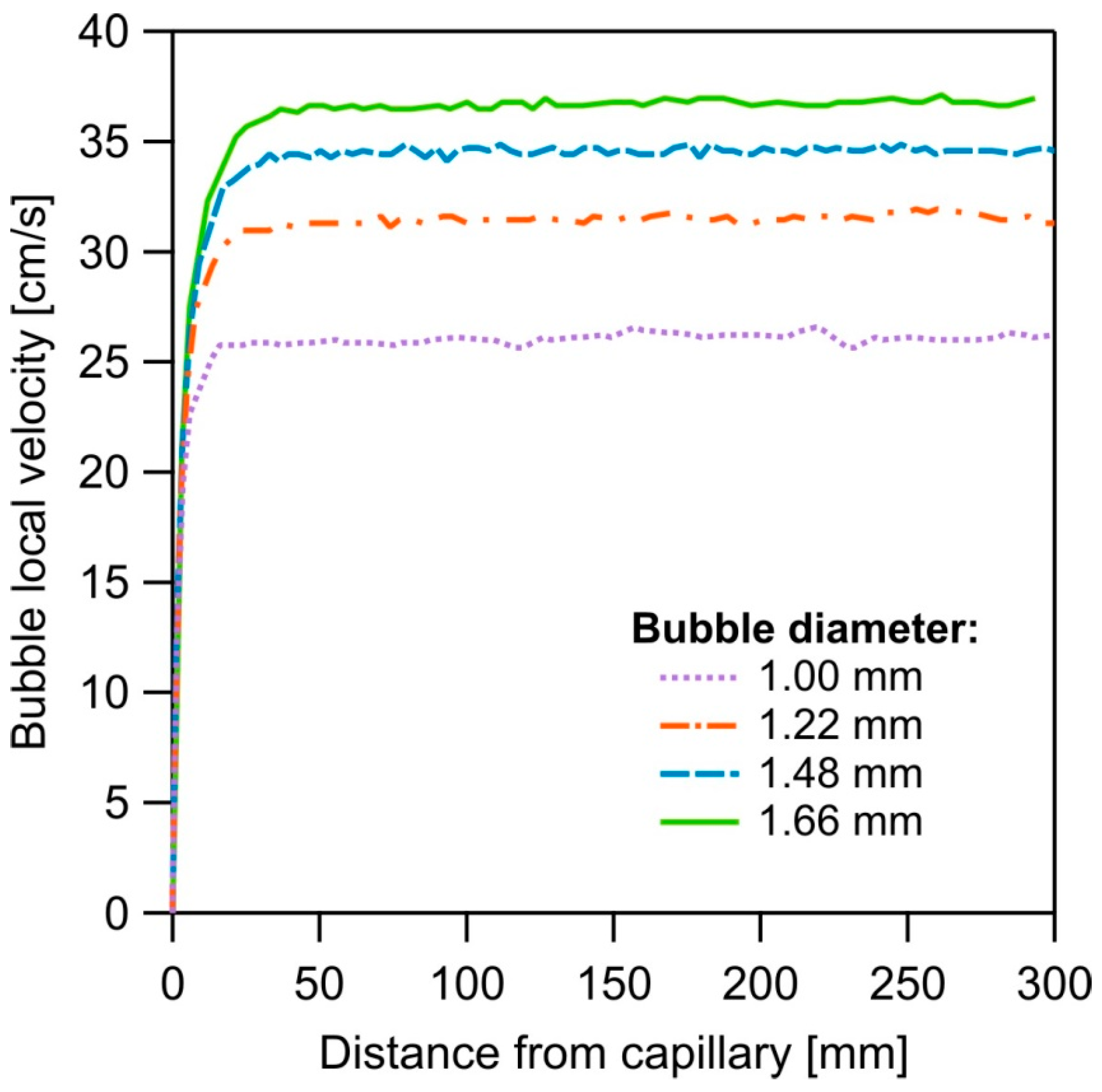
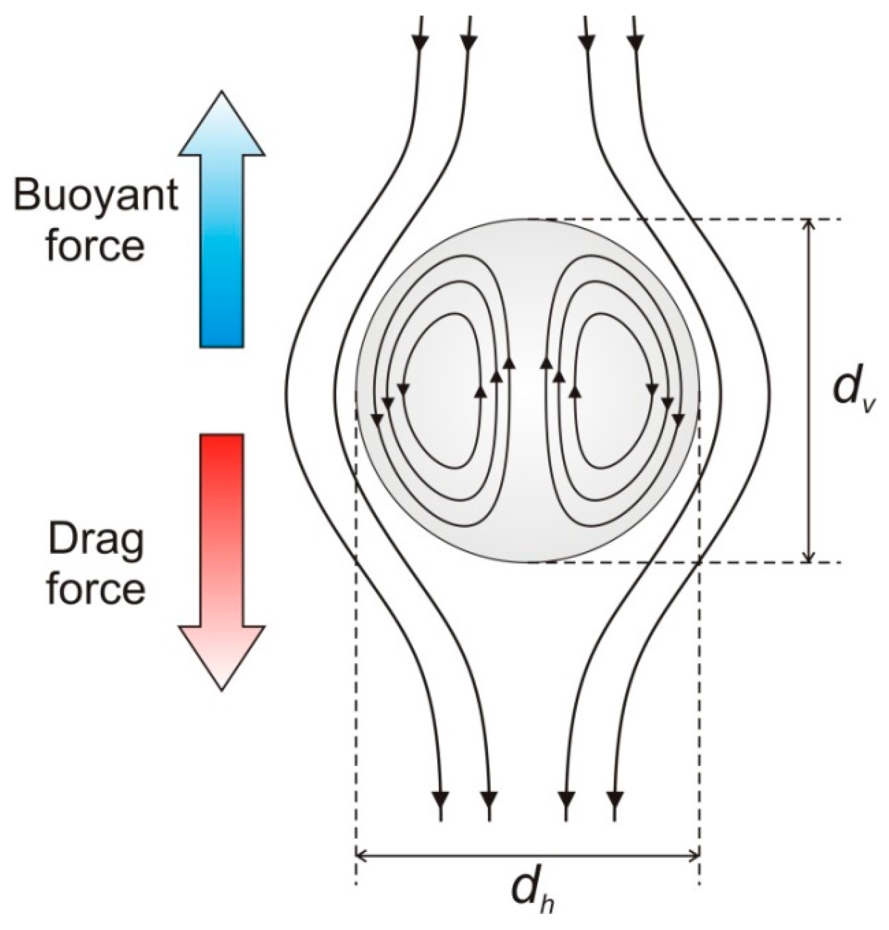
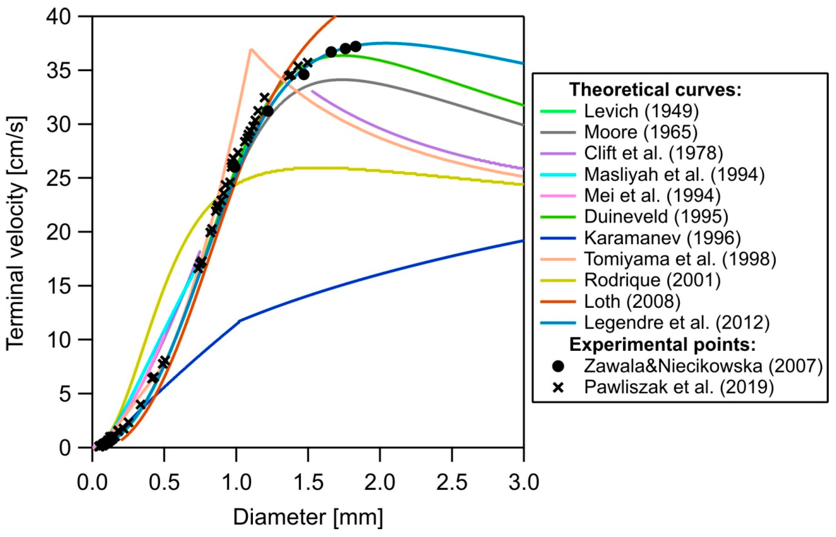
3. Bubble Motion in Pure Liquids

The motion (rising or falling) of a body in liquid with its terminal velocity (UT) is described by the balance between the buoyancy (FB) and the drag force (FD):
F B = Δ ρ V b g
F D = 0.5 C D ρ L U T 2 S b
where CD is the drag coefficient, ρL is the liquid density, and Vb and Sb are the volume and surface of projection on a horizontal plane of the body, respectively. Then, for a spherical body of the diameter db, the equation for terminal velocity can be expressed as:
U T = ( 4 d b Δ ρ g 3 C D ρ L ) 1 / 2
The main problem in the analytical solving of Equation (7) is the determination of the drag coefficient. The CD depends on the conditions of motion, often expressed as a function of the dimensionless Reynolds number (Re) [16]:
R e = d b U T ρ L η L
where ηL is the liquid viscosity. In fluid mechanics, the Reynolds number gives a measure of the ratio of inertial forces to viscous drag and is often used for the description of flow conditions. It is assumed that a bubble moves under creeping flow conditions when Re ≪ 1, a spherical regime for Re < 20, an ellipsoidal regime for 20 < Re < 4700, and a spherical or ellipsoidal cap regime for Re > 4700 [50].
The Reynolds number, together with the Morton (Mo) and Eovots (Eo) numbers are used for the characterization of the hydrodynamic conditions of the body motion in fluid. The Morton and Eovots (also called Bond) numbers present the shape of bubbles or drops moving in a surrounding fluid [16]:
M o = η L 4 g Δ ρ ρ L 2 σ 3
E o = d b 2 g Δ ρ σ
The other, often used, dimensionless numbers are the Weber (We), Archimedes (Ar), and Lyshchenko (Ly) numbers [16]:
W e = d b U T 2 Δ ρ σ
A r = d b 3 g Δ ρ ρ L η L 2
L y = U T 3 ρ L 2 g Δ ρ η L
In the case of a single bubble formed on a capillary orifice, two stages at the profile of the local velocity can be distinguished: (i) an acceleration stage, when the local velocity increases monotonically, and (ii) a terminal stage, when a constant value of the velocity is achieved. Figure 5 presents the local velocity profiles for bubbles of various diameters as a function of the distance from the capillary orifice. It can be observed that the bubble accelerates rapidly and, after ca. 30–40 mm (depending on the bubble size), the velocity of the bubble starts to be constant. The establishment of the terminal velocity is a consequence of the balance between the drag force and buoyancy.
One of the very first models of the CD, known as Stokes’ law, was obtained by solving the Navier–Stokes equation for a symmetrical solid sphere falling in liquid under creeping flow conditions [52]:
C D = 24 Re
which, together with Equations (7) and (8), gives:
U T = d b 2 g Δ ρ 18 η L
In the early 20th century, Hadamard [53] and Rybczynski [54] independently, showed that the terminal velocity of a fluid sphere is up to 50% higher than the velocity of a rigid sphere of the same size and density. This effect is related to the smaller viscous drag exerted by the liquid phase at the liquid–gas interface and the internal gas circulation induced inside a bubble, as presented schematically in Figure 6. Thus, the equation for terminal velocity takes the form [53,54]:
U T = d b 2 g Δ ρ 6 η L η L + η G 2 η L + 3 η G d b 2 g Δ ρ 12 η L
where ηG is the gas viscosity.
It is interesting to mention that Pawliszak et al. [56] showed that the terminal velocities of bubbles of 215–550 μm in diameter deviate from the theoretical ones predicted for a fully mobile water—air interface, while for bubbles of below 180 μm in diameter good compliance with the Stokes’ model is observed. This shift from full mobility to an immobile water—air interface is associated with the sensitivity of tiny (db < 500 μm) bubbles to any surface-active impurities in water. Vakarelski et al. [57] confirmed, by carrying out similar experiments in perfluorocarbon liquids, that for the clean continuous phase the bubble is at the mobile liquid—air interface, giving higher terminal velocity than that predicted by the Stokes’ law, which follows Equation (16).
Levich [58] and Ackeret [59] independently elaborated a model for the potential flow of spherical drops and bubbles in clean water, where the expression for the CD for Re < 50 and db < 0.5 mm is given as:
C D = 48 Re
Bubbles of large diameters have non-spherical shapes, which influences the drag coefficient. For such an oblate spheroid, Moore [20,21] obtained, considering the dissipation of energy on the boundary layer, the following relation of the CD:
C D = 48 R e G ( χ ) [ 1 + H ( χ ) R e + O ( 1 R e ) ]
where G(χ) and H(χ) are functions of the bubble deformation degree (χ):
G ( χ ) = 1 3 χ 4 / 3 ( χ 2 1 ) 3 / 2 χ 2 1 ( 2 χ 2 ) s 1 χ ( χ 2 s 1 χ χ 2 1 ) 2
H ( χ ) = 0.0195 χ 4 0.2134 χ 3 + 1.7026 χ 1.5732
Both functions, G(χ) and H(χ), were simplified for χ < 2 by Loth [50]:
G ( χ ) = 0.1287 + 0.4256 χ + 0.4466 χ 2
H ( χ ) = 0.8886 + 0.5693 χ 0.4563 χ 2
The deformation can be found from the relationship between the Weber number and χ. For small distortions, i.e., χ < 1.1, this is [21]:
χ = 1 + 9 64 W e + O ( W e 2 )
while, for moderate and great deformations (χ > 1.1):
W e = 4 χ 4 / 3 ( χ 3 + χ 2 ) ( χ 2 s 1 χ χ 2 1 ) 2 ( χ 2 1 ) 3
For χ < 2, Equations (23) and (24) can be approximated by a simple relationship:
χ = 1 + 9 64 W e 0.0089 W e 2 + 0.0287 W e 3
The Moore model [20,21] is said to be applicable for a wide range of the Reynolds number, 100 < Re < 10,000, but a comparison of the prediction with experimental data [16,60] showed that this model underestimates values of the bubble terminal velocities for bubbles of db > 1.2 mm. Thus, Duineveld [60] proposed the following formula:
χ = ( a 1 W e 0 W e ) 1 2
where We0 and a1 are 4.412 and 4.39, respectively. The main limitation of Equation (26) is that for WeWe0, the χ is increasing indefinitely.
Based on data for ultra-pure water over a range of Reynolds numbers from 0.2 to 5000, Loth [50] proposed an approximate correlation for the aspect ratio of ‘uncontaminated’ bubbles as:
χ = [ 1 ( 1 E min ) tanh ( c E W e ) ] 1
where:
E min = 0.250 + 0.55 exp ( 0.09 Re )
c E = 0.165 + 0.55 exp ( 0.30 Re )
Legendre et al. [19] proposed a simple formula closely describing the bubble deformation in water for χ < 3:
χ = ( 1 9 64 W e ) 1
In general, the Weber number, which is defined as the ratio of continuous-fluid stresses (causing deformation) to surface tension stresses (resisting deformation), describes bubble geometry qualitatively by the following relationships [50]:
  • We ≪ 1—bubble shape tends to a spherical geometry;
  • We ~ 1—moderate deviations, oblate spheroid is observed;
  • We ≫ 1—large bubble shape distortion occurs; spherical cap and oblate ellipsoidal cap are observed.
In their monograph, Clift et al. [16] reviewed most of the known models and compared them with experimental data. They emphasized the influence of bubble deformation on the drag coefficient for bubbles rising in clean water, which resulted in the presentation of two equations, for two separate regimes:
  • for Re < 150
C D = 14.9 R e 0.78
  • for Re > 565:
U T = ( 2.14 σ d b ρ L + 0.505 d b g ) 1 / 2
The other semi-analytical formula for the CD, which fits with experimental data for Re < 130 in clean water, was proposed by Masliyah et al. [61]:
C D = 16 R e ( 1 + 0.077 R e 0.65 )
After analyzing the available experimental data and the correlations for the motion of rising gas bubbles, Karamanev [62,63] proposed a semi-analytical equation linking the bubble rising velocity and its geometry. Moreover, the drag coefficient was described in a more convenient way—in terms of the Archimedes number (Ar). Using these considerations, the terminal velocity of the bubble can be calculated as follows:
U T = d e d h 4 g d b 3 C D
and the drag coefficient is expressed as:
C D = 432 A r ( 1 + 0.047 A r 2 / 3 ) + 0.517 1 + 154 A r 1 / 3
for Ar < 13,000, and CD = 0.95 for Ar > 13,000. The term de/dh is related to the changes in the bubble area projected on a horizontal plane, and can be calculated using the correlation proposed by Clift et al. [16]:
d e d h = ( 1 + 0.163 E o 0.757 ) 1 / 3
for Eo < 40, and de/dh = 0.62 for Eo > 40. This model does not take into account the fluidity of the liquid–air interface, giving rather poor predictions when compared with experimental data, as seen in Figure 7.
Subsequently, Mei et al. [64,65] proposed a theoretical prediction of the terminal velocity based on the numerical solution of their model for the unsteady motions of particles (including droplets and bubbles) in a carrier fluid. For Re < 50, the drag coefficient is given as [65]:
C D = 16 Re { 1 + [ 8 Re + 0.5 ( 1 + 3.315 Re 1 / 2 ) ] 1 }
Rodrigue [66,67] proposed another generalized correlation, which uses the flow number (Fl) and the velocity number (Ve) introduced earlier by Abou-El-Hassan [68]:
F l = g ( ρ L 5 d b 8 σ η L 4 ) 1 / 3
V e = U T ( ρ L 2 d b 2 σ η L ) 1 / 3
Based on the experimental data available, Rodrigue found the following relationship [69]:
V e = F l 12 [ ( 1 + 1.31 10 5 × M o 11 / 20 F l 73 / 33 ) 21 / 176 ( 1 + 0.020 F l 10 / 11 ) 10 / 11 ]
Figure 7. Terminal velocity of an air bubble rising in ultra-pure water as a function of the bubble diameter (points—experimental results [48,56], lines—theoretical models [16,19,20,21,50,55,60,61,63,64,65,66,67,70,71,72]).
Minerals 13 01130 g007
Figure 7 presents a comparison between experimental results and most of the described models within this review for the terminal velocity of bubbles rising in ultra-pure water. As can be seen, most of the models overestimate bubble velocities for db < 1.0 mm, while underestimating bubble velocities for db > 1.0 mm. A good agreement between the experimental data and the Moore model combined with the relationship between the Weber number and χ proposed by Legendre et al. [19] is observed.

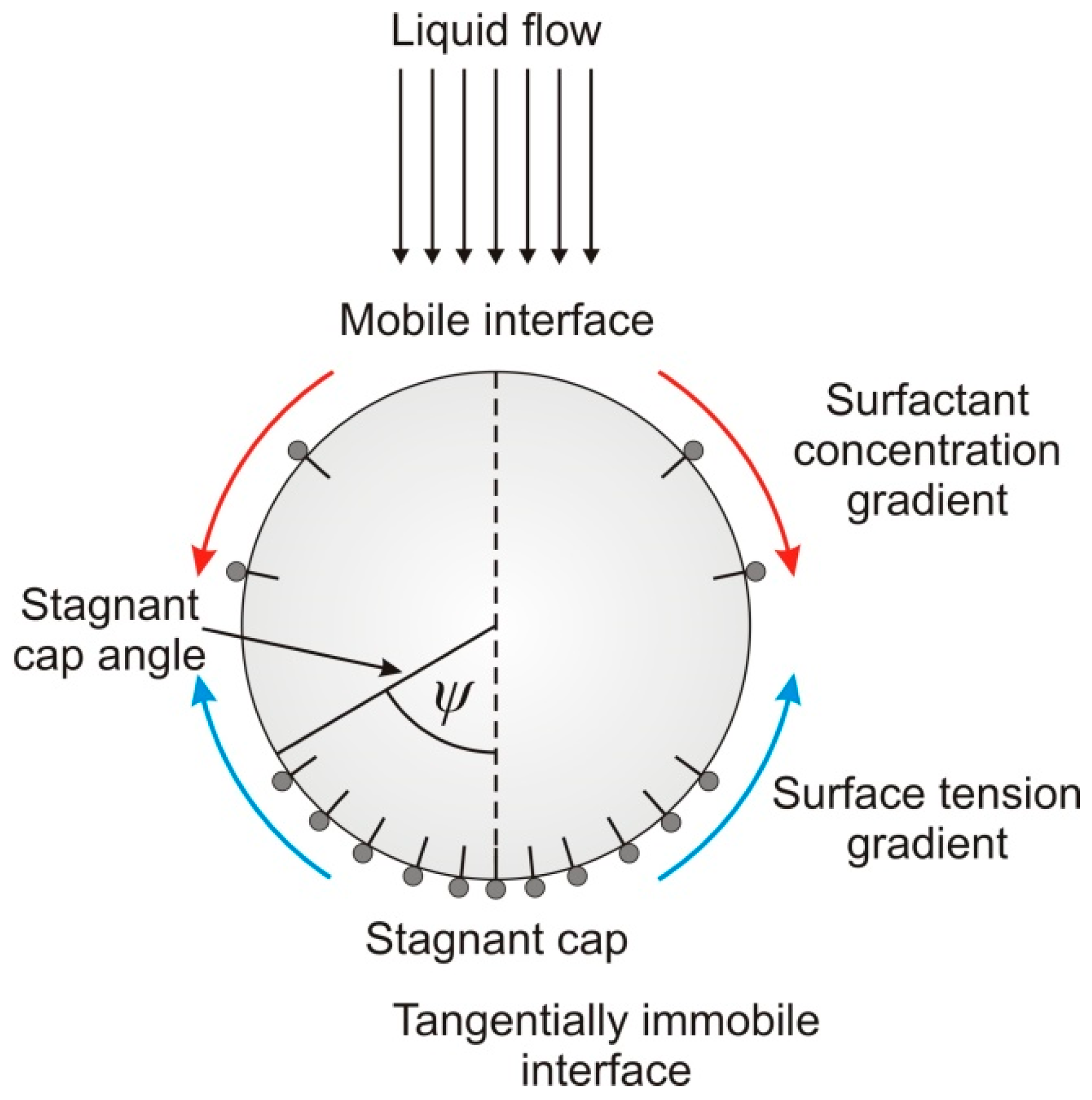
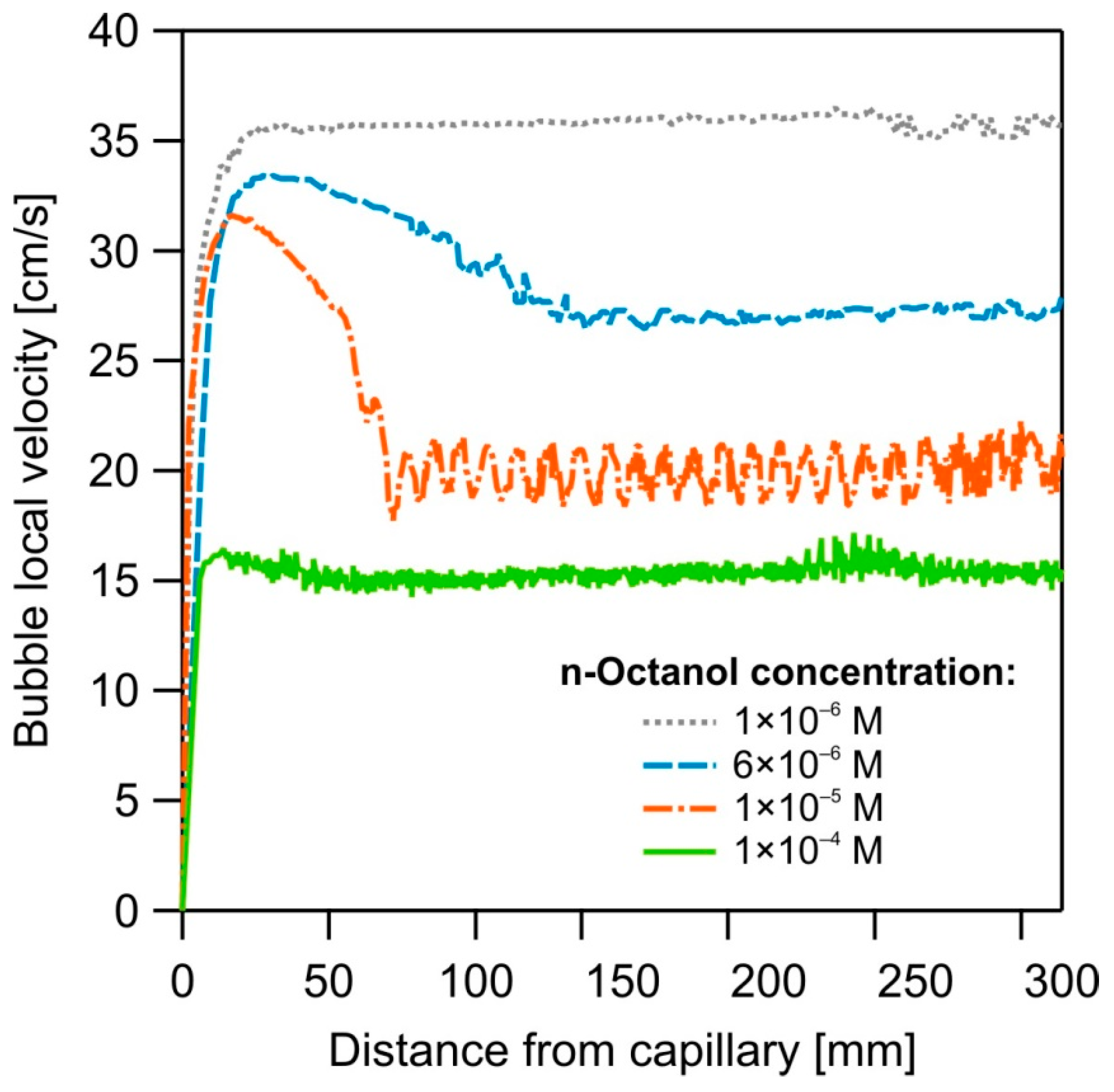
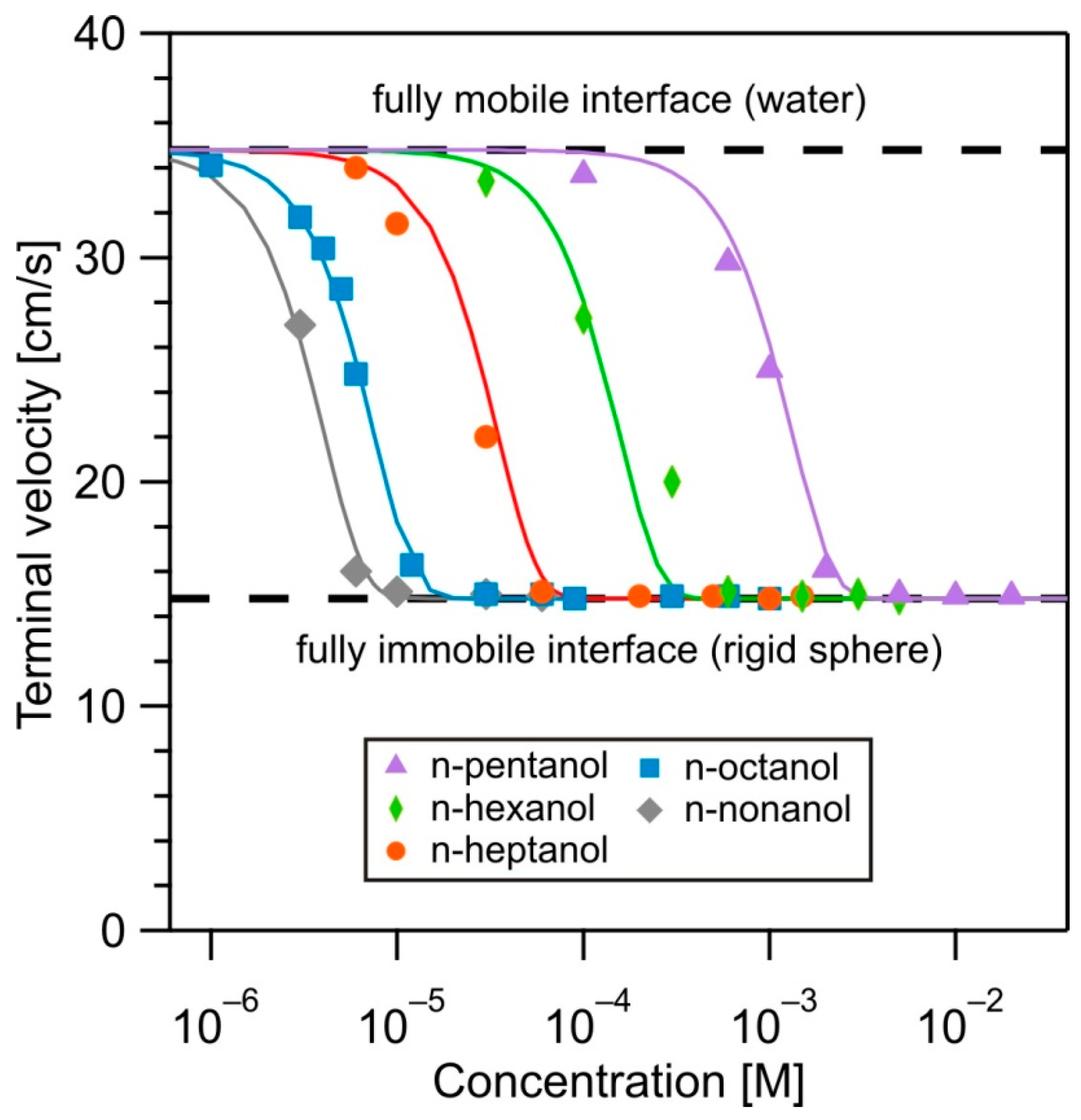
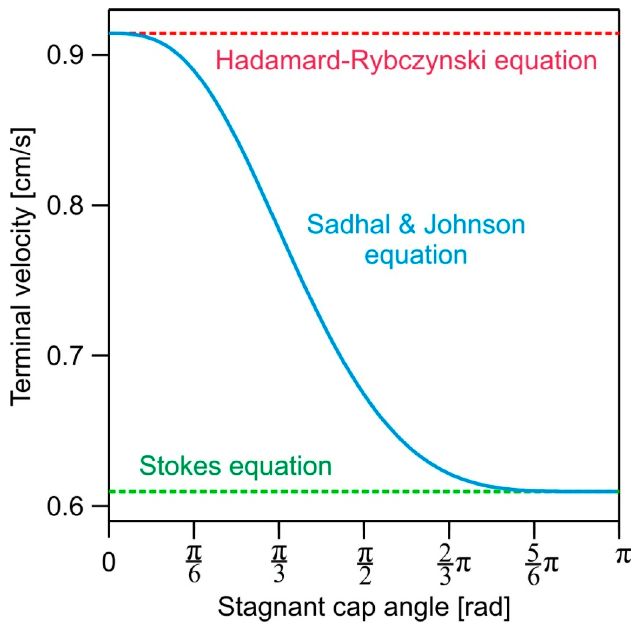
4. Bubble Motion in the Solution of a Surface-Active Substance

The presence of surface-active substances (SAS) and their adsorption at the bubble surface affect (retard) the fluidity of the surface, which leads to a lowering of the bubble velocity [49,73,74,75,76,77,78,79,80]. The mechanism responsible for this effect was described for the first time by Frumkin and Levich [55,81]. They postulated that a bubble detaching from a capillary has uniform adsorption coverage of the SAS molecules over its surface but viscous drag exerted by the liquid on the rising bubble surface induces the uneven distribution of the SAS molecules. Depletion at the upstream part of the bubble and accumulation of the SAS molecules in the rear part of the bubble results in an inducement of the surface tension gradients and a tangential ‘Marangoni’ stress opposing the flow shear stress (Figure 8) [81]. Thus, the formation of this dynamic adsorption layer over the bubble interface is the reason for the retardation of the bubble surface fluidity and internal circulation, which leads to an increase in the drag force towards that of a rigid sphere [82,83,84,85,86].
As seen in Figure 9, in a solution of SAS, up to four bubble motion stages can be determined [49,74,76,79,80]: (i) acceleration, (ii) maximum velocity, (iii) deceleration, and (iv) terminal velocity. All physicochemical parameters (e.g., the value of the initial acceleration, the height and width of the velocity maximum, the period of bubble deceleration and the distance (time) needed for terminal velocity establishment, and bubble shape pulsations) describing the motion of the bubble for each mentioned stage can be used to track the DAL development and the moment of the formation of its full architecture, causing the immobilization of the rising bubble (liquid–gas) interface.
The bubble, detached from the capillary orifice, accelerates and attains its terminal velocity at a distance, which is highly dependent on the type and concentration of SAS (Figure 9). Moreover, the existence of the acceleration/deceleration stage for some concentrations of SAS, before the establishment of the terminal velocity, can be addressed by the formation of the DAL architecture during the initial stage of the bubble motion [24,75,76].
There is also a minimum degree of adsorption coverage (concentration), different for various SAS, which is sufficient for the full immobilization of the bubble surface [24,75,76]. A further increase in the SAS coverage, above this ‘threshold’ coverage, does not practically affect the bubble terminal velocity, as seen in Figure 10. The full retardation of the bubble surface mobility means that its motion is similar to that of a solid sphere of identical dimensions and density.
The terminal velocity of the bubble in solutions of SAS, often called ‘contaminated’ liquids, was the topic of many research studies, mainly focused on bubbles with fully immobilized surfaces, whose motion showed some similarities to the falling of rigid spheres. In the case of a rise in the laminar flow conditions, the drag coefficient can be described using the Stokes equation (Equation (14)), but even for such small velocities, deviations, first noted by Oseen [87], were observed. Ossen, after simplifying the Navier–Stokes equation by linearization, showed that the drag coefficient becomes larger compared to Equation (14) and for Re < 0.1 it can be calculated from [87]:
C D = 24 R e ( 1 + 3 16 R e )
In the case of a higher Reynolds number (for Re < 800), Schiller and Naumann proposed the following formula [88]:
C D = 24 R e ( 1 + 0.15 R e 0.687 )
Clift et al. [16] collected and analyzed data for ‘contaminated’ liquids, similarly as for bubbles’ motion in pure liquids, and presented the following relationship for bubble terminal velocities:
U T = η L ρ L d b M o 0.149 ( J C 0.857 )
where:
J C = 0.94 H C 0.757
for 2 < HC < 59.3, and
J C = 3.42 H C 0.441
for HC > 59.3, and HC is described as:
H C = 4 3 E o M o 0.149
Karamanev [63] assumed that Equation (35), used for the clean water system, can be used for an estimation of the CD in the case of a free rising sphere in ‘contaminated’ liquids. If the bubble in ‘contaminated’ liquid has a spherical shape, then there is no need to add a geometrical term in the formula for bubble terminal velocity. Thus, the terminal velocity of a free rising sphere should be calculated from Equations (7) and (34) for Ar < 1.18·106db2, and CD = 0.95 for Ar > 1.18·106db2.
Nguyen et al. [89] also showed that the terminal velocity of a settling solid sphere can be directly predicted on the basis of the Archimedes and Lyaschenko numbers, but in a more straightforward way than that proposed by Karamanev [63]. Later, using a similar derivation [90], the formulas for bubble terminal velocity in the ‘contaminated’ system were presented. Nguyen [90] assumed that for Re < 130, the bubble’s shape is spherical and the bubble drag coefficient is equal to that of a solid particle. The following correlation for bubble terminal velocity was proposed:
U T = d b 2 g Δ ρ 18 η L [ 1 + A r / 96 ( 1 + 0.079 A r 0.749 ) 0.755 ] 1
When Ar is small, the second part of Equation (48) converges to unity, transforming the equation to the Stokes law.
For Re > 130, Nguyen [90] proposed, similarly to Karamanev, that CD = 0.95, but in their formula for the bubble terminal velocity there are additional numerical parameters (a,b) describing the shape of rising bubble:
U T = g η L ρ L 3 ( 4 a 2 M o 0.46 b 2.85 ) 1 / ( 2 2 b ) A r 2 b + 1 6 6 b
The values of a and b depend on the Archimedes number and they are collected in the work of Nguyen [90].
Ng et al. [91,92] predicted the CD with the use of the solution of the Oseen law, and for 0.2 < Re < 20,000 the following formula was derived:
C D = 24 R e ( 7 6 R e 0.15 + 0.02 R e )
Figure 11 presents comparisons of experimental data and the velocity values predicted from the models for bubble motion in clean and ‘contaminated’ water (i.e., in the presence of various SAS (n-pentanol, n-hexanol, n-octanol, n-nonanol, n-octyltrimethylammonium bromide (OTAB), and n-octylsulphate sodium salt (OctylS-Na)). The existing models describe relatively well the boundary cases (i.e., ultra-pure and fully ‘contaminated’ systems), while proper predictions for the UT for intermediate states (i.e., the case of the partial immobilization of the bubble surface) are not covered by the models proposed. This issue was addressed in the work of Davis and Acrivos [93]. They proposed a model for the creeping flow of a ‘contaminated’ bubble that postulates the existence of a stagnant cap over the rear of the bubble, the size of which influences the drag force acting on the rising bubble. Later, Sadhal and Johnson [94] derived an analytical solution for the spherical stagnant cap. In their model, the bottom part of the rising bubble is completely covered with SAS, resulting in a tangentially immobile air–liquid interface, while the top part is free of SAS, giving a fully mobile boundary condition. They proposed a simple formula for the drag force of a ‘contaminated’ bubble:
F D = 2 π d b η L [ 1 4 π ( 2 ψ + sin ψ sin 2 ψ 1 3 sin 3 ψ ) + 1 ]
where ψ is the stagnant cap angle (see Figure 8). For the limiting case of ultra-pure water, i.e., ψ = 0, Equation (50) gives the Hadamard–Rybczynski equation. Similarly, for a fully ‘contaminated’ bubble surface, i.e., ψ = π, Equation (50) transforms into the Stokes equation.
Figure 12 presents bubble terminal velocity calculated using the Sadhal and Johnson model [94] for an air bubble of a diameter equal to 0.1 mm. Assuming that the stagnant cap angle reflects the adsorption coverage, which is related to SAS concentration, then qualitative similarity to data, presented in Figure 10, especially theoretical lines, is seen. Unfortunately, a simple quantitative relationship between SAS adsorption coverage and the size of the stagnant cap is not available in the form of a direct analytical equation and needs to be calculated using numerical procedures [83,85].
Tomiyama et al. [70,71,72] proposed a different approach to the problem of the ‘contaminated’ system. Based on the previous works of Peebles and Garber [95] and Ishii and Chawla [96], they proposed formulas of the CD for three ‘contamination’ regimes:
(A)
for a clean system
C D = m a x { m i n [ 16 R e ( 1 + 0.15 R e 0.687 ) , 48 R e ] , 8 3 E o E o + 4 }
(B)
for a slightly ‘contaminated’ system
C D = m a x { m i n [ 24 R e ( 1 + 0.15 R e 0.687 ) , 72 R e ] , 8 3 E o E o + 4 }
(C)
for a fully ‘contaminated’ system
C D = m a x { 24 R e ( 1 + 0.15 R e 0.687 ) , 8 3 E o E o + 4 }
However, the conditions for a partially ‘contaminated’ system are not clearly described in the paper of Tomiyama et al. [70,71,72]. It is specified that a fully ‘contaminated’ bubble reaches its terminal velocities after covering a distance less than 17 mm from the point of bubble formation [71].
Yan et al. [97] made an attempt to deliver a single equation covering a wide range of fluid parameters (10−3 < Re < 105, 10−2 < Eo < 103, and 10−14 < Mo < 107) for a bubble rising in both pure and ‘contaminated’ liquids. Using nonlinear fitting to the experimental data, they proposed the following correlation:
C D = m a x { min [ 24 R e ( 1 + 0.15 R e 0.687 ) , 72 Re ] , 24 R e ( 1 + 0.15 R e 0.687 ) Re 0.55 E o 0.95 W e 1.10 12.6 ( M o M o * ) 0.048 }
where Mo* is the Mo of water at 293 K (2.6 × 10⁻¹¹).
Based on an analysis of the literature and experimental data for surfactants used as flotation frothers, Kowalczuk et al. [22] introduced the determination of a concentration at the minimum bubble velocity (CMV). Their empirical model allows us to predict the bubble terminal velocity as a function of the surfactant concentration (c) for a wide range of bubble diameters:
U T = U min + ( U max U min ) e 3 ( c / C M V ) 2
In this model, it is necessary to know the maximum (Umax) and minimum (Umin) terminal velocities, as well as the value of the CMV. For the most popular surface active substances, the CMV data are collected in the paper [22]. The values of Umax and Umin can also be estimated using models for bubbles with fully mobile (pure liquid) and fully immobile (rigid sphere) interfaces, respectively.

5. Limitations and Future Directions

Most of the presented models are either empirical, semi-analytical, or analytical solutions derived with many simplifying assumptions. More sophisticated models of bubble motion in solutions of surface-active substance require the numerical solution of the Navier–Stokes equation [82,98], mainly with the implementation of the rear stagnant cap model [73,94,99,100,101] and a finite-rate mass exchange between the interface and bulk fluid [82,83,102,103,104]. Similarly, models describing the motion of a bubble in a stagnant liquid have a limited application in technological processes, where a gas–liquid flow is turbulent [18,105,106]. In such conditions, bubbles tend towards coalescences, breakups, and deformations [16,107,108,109]. Moreover, the motion of a bubble is characterized by its instability with continuous acceleration and deceleration stages [110,111,112]. The prediction of bubble motion becomes even more complicated for bubble swarms (groups of bubbles dispersed in a liquid phase), which are typical for industrial processes [113,114,115]. In this situation, advanced numerical methods, i.e., computational fluid dynamics (CFD), need to be implemented [116]. Particular attention should be paid to two CFD methods: direct numerical solutions (DNS) [112,117] and discrete element methods (DEM) [118]. The former technique allows us to resolve the turbulent fluid motion [119,120], but the price is high: most of the time it demands a computing power which can be assured by supercomputers only [120]. The discrete element method, which is less demanding in terms of computing resources, is implemented in the study of bubble–solid particles interactions, especially in terms of flotation processes [121,122,123,124]. The further development of DNS and DEM is rather inevitable, as both methods deliver significant and often satisfactory outcomes.

6. Conclusions

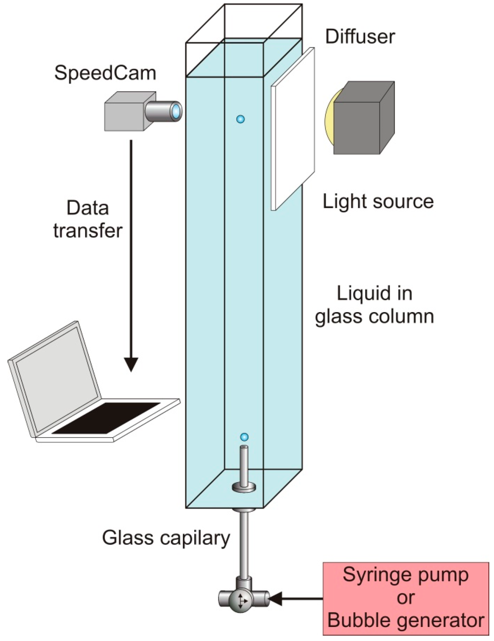
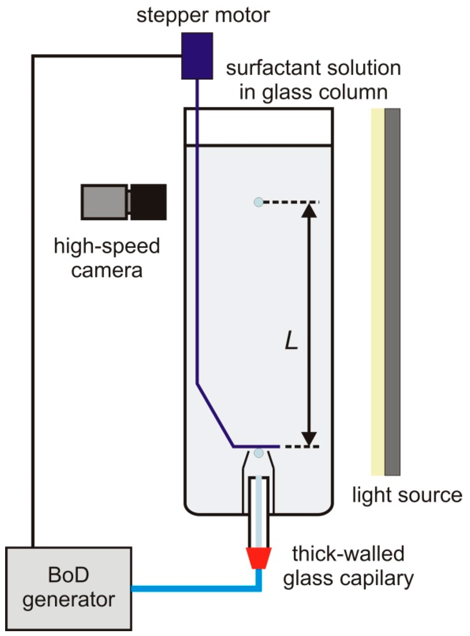
  • Experimental methods to study bubble motion: visual observation (with use of cameras) is still the most reliable method for tracking bubbles. This method delivers the most comprehensive information about bubble motion, i.e., velocity, deformation, and path.
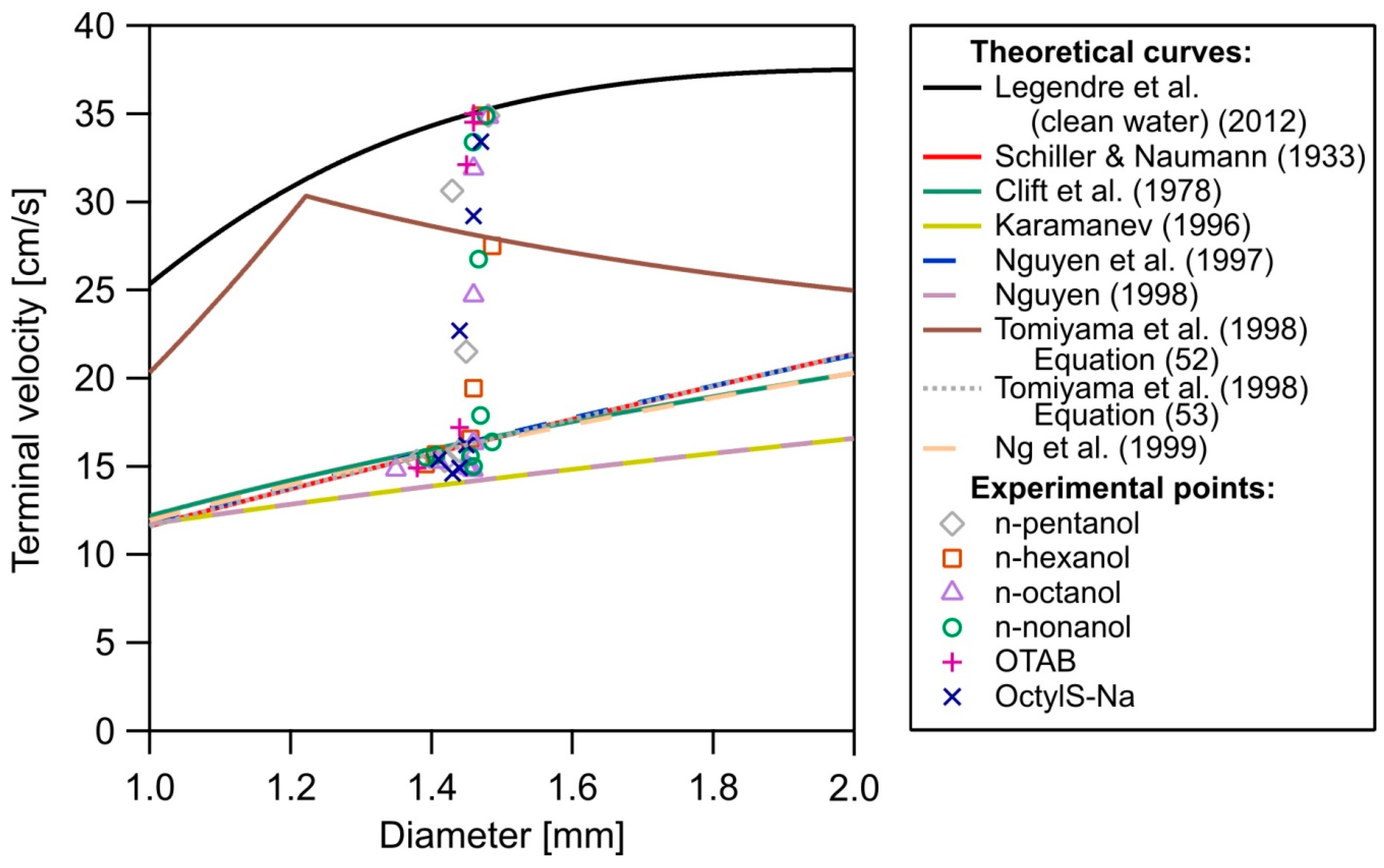
  • Bubble motion in water: it was shown that predictions of the model proposed by Moore [20,21], supplemented by recent semi-empirical formulas (Legendre et al. [19]) describing the geometrical parameters of the rising bubble (deformation ratio), agree almost perfectly with experimental data for pure liquids.
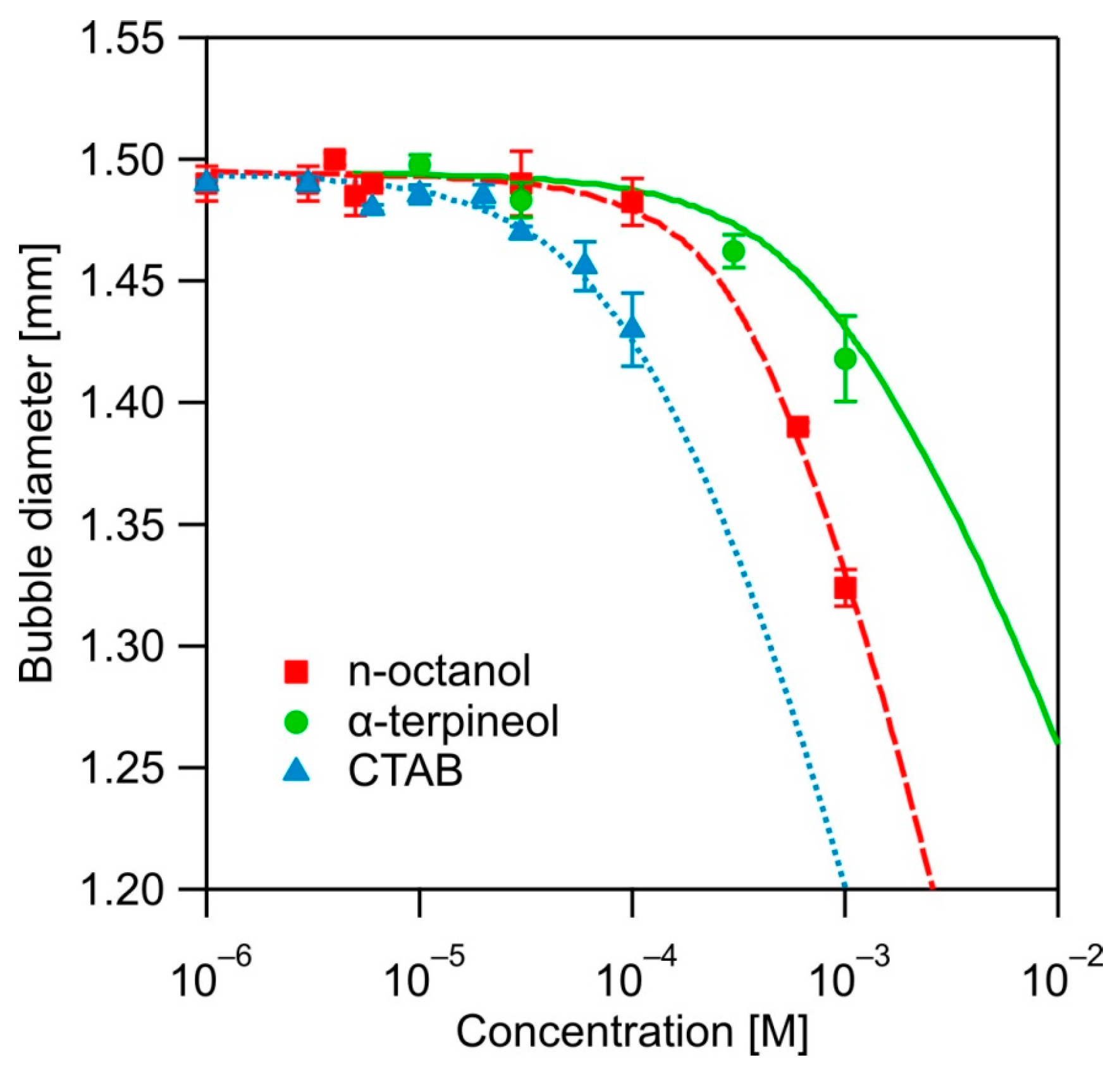
  • Bubble motion in liquid in the presence of surface-active substances (SAS): for SAS solutions, existing models describe relatively well the boundary case of fully ‘contaminated’ systems. It was shown that the semi-empirical model proposed by Kowalczuk et al. [22] is a very convenient tool for the description and prediction of bubble terminal velocities as a function of surfactant concentration for a wide range of bubble diameters.

Author Contributions

Conceptualization, D.K., A.W.-P., P.B.K. and J.Z.; software, D.K. and J.Z.; validation D.K. and A.W.-P.; formal analysis, D.K. and A.W.-P.; data curation, D.K., P.B.K. and J.Z.; writing—original draft preparation, D.K.; writing—review and editing, D.K., A.W.-P., P.B.K. and J.Z.; visualization, D.K. and A.W.-P.; supervision, P.B.K. and J.Z.; project administration, J.Z.; funding acquisition, J.Z. All authors have read and agreed to the published version of the manuscript.

Funding

This research was funded by Polish National Science Centre (NCN) grant number 2021/43/B/ST8/00053.

Data Availability Statement

Data available on request.

Acknowledgments

Partial financial support from the Polish National Science Centre (NCN grant no. 2021/43/B/ST8/00053) is acknowledged with gratitude.

Conflicts of Interest

The authors declare no conflict of interest.

References

  1. Leja, J. Surface Chemistry of Froth Flotation; Plenum Press: New York, NY, USA; London, UK, 1982. [Google Scholar]
  2. Nguyen, A.V.; Schulze, H.J. Colloidal Science of Flotation; Surfactant Science; CRC Press: Boca Raton, FL, USA, 2004. [Google Scholar]
  3. Nguyen, A.V.; Schulze, H.J.; Ralston, J. Elementary Steps in Particle-Bubble Attachment. Int. J. Miner. Process. 1997, 51, 183–195. [Google Scholar] [CrossRef]
  4. Fuerstenau, D.W. Pradip Zeta Potentials in the Flotation of Oxide and Silicate Minerals. Adv. Colloid Interface Sci. 2005, 114, 9–26. [Google Scholar] [CrossRef] [PubMed]
  5. Drzymala, J. Characterization of Materials by Hallimond Tube Flotation. Part 1: Maximum Size of Entrained Particles. Int. J. Miner. Process. 1994, 42, 139–152. [Google Scholar] [CrossRef]
  6. Zawala, J.; Drzymala, J.; Malysa, K. Natural Hydrophobicity and Flotation of Fluorite. Physicochem. Probl. Miner. Process. 2007, 41, 5–11. [Google Scholar]
  7. Firouzi, M.; Nguyen, A.V.; Hashemabadi, S.H. The Effect of Microhydrodynamics on Bubble–Particle Collision Interaction. Miner. Eng. 2011, 24, 973–986. [Google Scholar] [CrossRef]
  8. Brabcová, Z.; Karapantsios, T.; Kostoglou, M.; Basařová, P.; Matis, K. Bubble–Particle Collision Interaction in Flotation Systems. Colloids Surf. A Physicochem. Eng. Asp. 2015, 473, 95–103. [Google Scholar] [CrossRef]
  9. Xing, Y.; Gui, X.; Pan, L.; Pinchasik, B.-E.; Cao, Y.; Liu, J.; Kappl, M.; Butt, H.-J. Recent Experimental Advances for Understanding Bubble-Particle Attachment in Flotation. Adv. Colloid Interface Sci. 2017, 246, 105–132. [Google Scholar] [CrossRef]
  10. Drzymala, J. Mineral Processing, Foundations of Theory and Practice of Minerallurgy; Oficyna Wydawnicza PWr.: Wroclaw, Poland, 2007. [Google Scholar]
  11. Grau, R.A.; Laskowski, J.S.; Heiskanen, K. Effect of Frothers on Bubble Size. Int. J. Miner. Process. 2005, 76, 225–233. [Google Scholar] [CrossRef]
  12. Melo, F.; Laskowski, J.S. Fundamental Properties of Flotation Frothers and Their Effect on Flotation. Miner. Eng. 2006, 19, 766–773. [Google Scholar] [CrossRef]
  13. Laskowski, J.S. A New Approach to Classification of Flotation Collectors. Can. Metall. Q. 2010, 49, 397–404. [Google Scholar] [CrossRef]
  14. Ralston, J. Thin Films and Froth Flotation. Adv. Colloid Interface Sci. 1983, 19, 1–26. [Google Scholar] [CrossRef]
  15. Albijanic, B.; Ozdemir, O.; Nguyen, A.V.; Bradshaw, D. A Review of Induction and Attachment Times of Wetting Thin Films between Air Bubbles and Particles and Its Relevance in the Separation of Particles by Flotation. Adv. Colloid Interface Sci. 2010, 159, 1–21. [Google Scholar] [CrossRef]
  16. Clift, R.; Grace, J.R.; Weber, M.E. Bubbles, Drops, and Particles; Academic Press: New York, NY, USA, 1978. [Google Scholar]
  17. Kulkarni, A.A.; Joshi, J.B. Bubble Formation and Bubble Rise Velocity in Gas−Liquid Systems:  A Review. Ind. Eng. Chem. Res. 2005, 44, 5873–5931. [Google Scholar] [CrossRef]
  18. Chen, Y.; Wang, L.; Chang, H.; Zhang, Q. A Review of Drag Coefficient Models in Gas-Liquid Two-Phase Flow. ChemBioEng Rev. 2023, 10, 311–325. [Google Scholar] [CrossRef]
  19. Legendre, D.; Zenit, R.; Velez-Cordero, J.R. On the Deformation of Gas Bubbles in Liquids. Phys. Fluids 2012, 24, 043303. [Google Scholar] [CrossRef]
  20. Moore, D.W. The Boundary Layer on a Spherical Gas Bubble. J. Fluid Mech. 1963, 16, 161–176. [Google Scholar] [CrossRef]
  21. Moore, D.W. The Velocity of Rise of Distorted Gas Bubbles in a Liquid of Small Viscosity. J. Fluid Mech. 1965, 23, 749–766. [Google Scholar] [CrossRef]
  22. Kowalczuk, P.B.; Zawala, J.; Drzymala, J. Concentration at the Minimum Bubble Velocity (CMV) for Various Types of Flotation Frothers. Minerals 2017, 7, 118. [Google Scholar] [CrossRef]
  23. Zawala, J.; Swiech, K.; Malysa, K. A Simple Physicochemical Method for Detection of Organic Contaminations in Water. Colloids Surf. A Physicochem. Eng. Asp. 2007, 302, 293–300. [Google Scholar] [CrossRef]
  24. Malysa, K.; Krasowska, M.; Krzan, M. Influence of Surface Active Substances on Bubble Motion and Collision with Various Interfaces. Adv. Colloid Interface Sci. 2005, 114, 205–225. [Google Scholar] [CrossRef]
  25. Saffman, P.G. On the Rise of Small Air Bubbles in Water. J. Fluid Mech. 1956, 1, 249–275. [Google Scholar] [CrossRef]
  26. Brücker, C. Structure and Dynamics of the Wake of Bubbles and Its Relevance for Bubble Interaction. Phys. Fluids 1999, 11, 1781–1796. [Google Scholar] [CrossRef]
  27. Mougin, G.; Magnaudet, J. Wake-Induced Forces and Torques on a Zigzagging/Spiralling Bubble. J. Fluid Mech. 2006, 567, 185–194. [Google Scholar] [CrossRef]
  28. Ju, E.; Cai, R.; Sun, H.; Fan, Y.; Chen, W.; Sun, J. Dynamic Behavior of an Ellipsoidal Bubble Contaminated by Surfactant near a Vertical Wall. Korean J. Chem. Eng. 2022, 39, 1165–1181. [Google Scholar] [CrossRef]
  29. Lunde, K.; Perkins, R.J. Shape Oscillations of Rising Bubbles. Appl. Sci. Res. 1997, 58, 387–408. [Google Scholar] [CrossRef]
  30. Zhang, T.; Qian, Y.; Yin, J.; Zhang, B.; Wang, D. Experimental Study on 3D Bubble Shape Evolution in Swirl Flow. Exp. Therm. Fluid Sci. 2019, 102, 368–375. [Google Scholar] [CrossRef]
  31. Luo, Y.; Wang, Z.; Zhang, B.; Guo, K.; Zheng, L.; Xiang, W.; Liu, H.; Liu, C. Experimental Study of the Effect of the Surfactant on the Single Bubble Rising in Stagnant Surfactant Solutions and a Mathematical Model for the Bubble Motion. Ind. Eng. Chem. Res. 2022, 61, 9514–9527. [Google Scholar] [CrossRef]
  32. Borkowski, M.; Zawala, J. Influence of Temperature on Rising Bubble Dynamics in Water and N-Pentanol Solutions. Minerals 2021, 11, 1067. [Google Scholar] [CrossRef]
  33. Malysa, K. Wet Foams: Formations, Properties and Mechanical Stability. Adv. Colloid Interface Sci. 1992, 40, 37–83. [Google Scholar] [CrossRef]
  34. Cho, Y.S.; Laskowski, J.S. Bubble Coalescence and Its Effect on Dynamic Foam Stability. Can. J. Chem. Eng. 2002, 80, 299–305. [Google Scholar] [CrossRef]
  35. Cho, Y.S.; Laskowski, J.S. Effect of Flotation Frothers on Bubble Size and Foam Stability. Int. J. Miner. Process. 2002, 64, 69–80. [Google Scholar] [CrossRef]
  36. Kowalczuk, P.B. Determination of Critical Coalescence Concentration and Bubble Size for Surfactants Used as Flotation Frothers. Ind. Eng. Chem. Res. 2013, 52, 11752–11757. [Google Scholar] [CrossRef]
  37. Tate, T. On the Magnitude of a Drop of Liquid Formed under Different Circumstances. Philos. Mag. 1864, 27, 176–180. [Google Scholar] [CrossRef]
  38. Kosior, D. Nanostructures and Stability of Thin Liquid Layers. Ph.D. Thesis, Jerzy Haber Institute of Catalysis and Surface Chemistry, Polish Academy of Sciences, Krakow, Poland, 2013. [Google Scholar]
  39. Oguz, H.N.; Prosperetti, A. Dynamics of Bubble Growth and Detachment from a Needle. J. Fluid Mech. 1993, 257, 111–145. [Google Scholar] [CrossRef]
  40. Garstecki, P.; Gitlin, I.; DiLuzio, W.; Whitesides, G.M.; Kumacheva, E.; Stone, H.A. Formation of Monodisperse Bubbles in a Microfluidic Flow-Focusing Device. Appl. Phys. Lett. 2004, 85, 2649–2651. [Google Scholar] [CrossRef]
  41. Martinez, C.J. Bubble Generation in Microfluidic Devices. Bubble Sci. Eng. Technol. 2009, 1, 40–52. [Google Scholar] [CrossRef]
  42. Niecikowska, A.; Krasowska, M.; Ralston, J.; Malysa, K. Role of Surface Charge and Hydrophobicity in the Three-Phase Contact Formation and Wetting Film Stability under Dynamic Conditions. J. Phys. Chem. C 2012, 116, 3071–3078. [Google Scholar] [CrossRef]
  43. Wielhorski, Y.; Abdelwahed, A.B.; Arquis, E.; Glockner, S.; Bréard, J. Numerical Simulation of Bubble Formation and Transport in Cross-Flowing Streams. J. Comput. Multiph. Flows. 2014, 6, 299–312. [Google Scholar] [CrossRef]
  44. Fu, T.; Ma, Y. Bubble Formation and Breakup Dynamics in Microfluidic Devices: A Review. Chem. Eng. Sci. 2015, 135, 343–372. [Google Scholar] [CrossRef]
  45. Vejražka, J.; Fujasová, M.; Stanovsky, P.; Ruzicka, M.C.; Drahoš, J. Bubbling Controlled by Needle Movement. Fluid Dyn. Res. 2008, 40, 521–533. [Google Scholar] [CrossRef]
  46. Sanada, T.; Abe, K. Generation of Single Bubbles of Various Sizes Using a Slitting Elastic Tube. Rev. Sci. Instrum. 2013, 84, 085106. [Google Scholar] [CrossRef]
  47. Najafi, A.S.; Xu, Z.; Masliyah, J. Single Micro-Bubble Generation by Pressure Pulse Technique. Chem. Eng. Sci. 2008, 63, 1779–1787. [Google Scholar] [CrossRef]
  48. Zawala, J.; Niecikowska, A. “Bubble-on-Demand” Generator with Precise Adsorption Time Control. Rev. Sci. Instrum. 2017, 88, 095106. [Google Scholar] [CrossRef] [PubMed]
  49. Kosior, D.; Zawala, J. Initial Degree of Detaching Bubble Adsorption Coverage and the Kinetics of Dynamic Adsorption Layer Formation. Phys. Chem. Chem. Phys. 2018, 20, 2403–2412. [Google Scholar] [CrossRef] [PubMed]
  50. Loth, E. Quasi-Steady Shape and Drag of Deformable Bubbles and Drops. Int. J. Multiph. Flow 2008, 34, 523–546. [Google Scholar] [CrossRef]
  51. Zawala, J. Formation and Rupture of Liquid Films Formed at Various Interfaces by the Colliding Bubble. Ph.D. Thesis, Jerzy Haber Institute of Catalysis and Surface Chemistry Polish Academy of Sciences, Krakow, Poland, 2008. [Google Scholar]
  52. Stokes, G.G. On the Effect of the Internal Friction of Fluids on the Motion of Pendulums. Trans. Camb. Philos. Soc. 1851, 9, 9–106. [Google Scholar]
  53. Hadamard, J.S. Mouvement Permanent Lent d’une Sphère Liquide et Visqueuse Dans Un Liquide Visqueux. Compt. Rend. Acad. Sci. 1911, 152, 1735–1752. [Google Scholar]
  54. Rybczynski, W. On the Translatory Motion of a Fluid Sphere in a Viscous Medium. Bull. Int. Acad. Sci. Crac. Sci. Math. Nat. 1911, Series A, 40–46. [Google Scholar]
  55. Levich, V.G. Physicochemical Hydrodynamics; Prentice-Hall Inc.: Englewood Cliffs, NJ, USA, 1962. [Google Scholar]
  56. Pawliszak, P.; Ulaganathan, V.; Bradshaw-Hajek, B.H.; Manica, R.; Beattie, D.A.; Krasowska, M. Mobile or Immobile? Rise Velocity of Air Bubbles in High-Purity Water. J. Phys. Chem. C 2019, 123, 15131–15138. [Google Scholar] [CrossRef]
  57. Vakarelski, I.U.; Manica, R.; Li, E.Q.; Basheva, E.S.; Chan, D.Y.C.; Thoroddsen, S.T. Coalescence Dynamics of Mobile and Immobile Fluid Interfaces. Langmuir 2018, 34, 2096–2108. [Google Scholar] [CrossRef]
  58. Levich, V.G. Motion of Gaseous Bubbles with High Reynolds Numbers. Zhn. Eksp. Teor. Fiz 1949, 19, 18–24. (In Russian) [Google Scholar]
  59. Ackeret, J. Über exakte Lösungen der Stokes-Navier-Gleichungen inkompressibler Flüssigkeiten bei veränderten Grenzbedingungen. J. Appl. Math. Phys. (ZAMP) 1952, 3, 259–271. [Google Scholar] [CrossRef]
  60. Duineveld, P.C. The Rise Velocity and Shape of Bubbles in Pure Water at High Reynolds Number. J. Fluid Mech. 1995, 292, 325–332. [Google Scholar] [CrossRef]
  61. Masliyah, J.; Jauhari, R.; Gray, M. Drag Coefficients for Air Bubble Rising along an Inclined Surface. Chem. Eng. Sci. 1994, 49, 1905–1911. [Google Scholar] [CrossRef]
  62. Karamanev, D.G. Rise of Gas Bubbles in Quiescent Liquids. AIChE J. 1994, 40, 1418–1421. [Google Scholar] [CrossRef]
  63. Karamanev, D.G. Equations for Calculations of the Terminal Velocity and Drag Coefficient of Solid Spheres and Gas Bubbles. Chem. Eng. Commun. 1996, 147, 75–84. [Google Scholar] [CrossRef]
  64. Mei, R.; Klausner, J.F. Unsteady Force on a Spherical Bubble at Finite Reynolds Number with Small Fluctuations in the Free-stream Velocity. Phys. Fluids A Fluid Dyn. 1992, 4, 63–70. [Google Scholar]
  65. Mei, R.; Klausner, J.F.; Lawrence, C.J. A Note on the History Force on a Spherical Bubble at Finite Reynolds Number. Phys. Fluids 1994, 6, 418–420. [Google Scholar] [CrossRef]
  66. Rodrigue, D. Drag Coefficient-Reynolds Number Transition for Gas Bubbles Rising Steadily in Viscous Fluids. Can. J. Chem. Eng. 2001, 79, 119–123. [Google Scholar]
  67. Rodrigue, D. Generalized Correlation for Bubble Motion. AIChE J. 2001, 47, 39–44. [Google Scholar]
  68. Abou-El-Hassan, M.E. A Generalized Bubble Rise Velocity Correlation. Chem. Eng. Commun. 1983, 22, 243–250. [Google Scholar]
  69. Rodrigue, D. A General Correlation for the Rise Velocity of Single Gas Bubbles. Can. J. Chem. Eng. 2004, 82, 382–386. [Google Scholar]
  70. Tomiyama, A.; Kataoka, I.; Zun, I.; Sakaguchi, T. Drag Coefficient of Single Bubbles under Normal and Micro Gravity Conditions. JSME Int. J. B Fluids Therm. Eng. 1998, 41, 472–479. [Google Scholar]
  71. Tomiyama, A.; Celata, G.P.; Hosokawa, S.; Yoshida, S. Terminal Velocity of Single Bubbles in Surface Tension Force Dominant Regime. Int. J. Multiph. Flow 2002, 28, 1497–1519. [Google Scholar]
  72. Myint, W.; Hosokawa, S.; Tomiyama, A. Terminal Velocity of Single Drops in Stagnant Liquid. J. Fluid Sci. Technol. 2006, 1, 72–81. [Google Scholar]
  73. Fdhila, R.B.; Duineveld, P.C. The Effect of Surfactant on the Rise of a Spherical Bubble at High Reynolds and Peclet Numbers. Phys. Fluids 1996, 8, 310–321. [Google Scholar]
  74. Sam, A.; Gomez, C.O.; Finch, J.A. Axial Velocity Profiles of Single Bubbles in Water/Frother Solutions. Int. J. Miner. Process. 1996, 47, 177–196. [Google Scholar]
  75. Krzan, M.; Malysa, K. Profiles of Local Velocities of Bubbles in N-Butanol, n-Hexanol and n-Nonanol Solutions. Colloids Surf. A Physicochem. Eng. Asp. 2002, 207, 279–291. [Google Scholar]
  76. Krzan, M.; Zawala, J.; Malysa, K. Development of Steady State Adsorption Distribution over Interface of a Bubble Rising in Solutions of N-Alkanols (C5, C8) and n-Alkyltrimethylammonium Bromides (C8, C12, C16). Colloids Surf. A Physicochem. Eng. Asp. 2007, 298, 42–51. [Google Scholar]
  77. Navarra, A.; Acuna, C.; Finch, J.A. Impact of Frother on the Terminal Velocity of Small Bubbles. Int. J. Miner. Process. 2009, 91, 68–73. [Google Scholar]
  78. Rafiei, A.A.; Robbertze, M.; Finch, J.A. Gas Holdup and Single Bubble Velocity Profile. Int. J. Miner. Process. 2011, 98, 89–93. [Google Scholar]
  79. Ulaganathan, V.; Krzan, M.; Lotfi, M.; Dukhin, S.S.; Kovalchuk, V.I.; Javadi, A.; Gunes, D.Z.; Gehin-Delval, C.; Malysa, K.; Miller, R. Influence of β-Lactoglobulin and Its Surfactant Mixtures on Velocity of the Rising Bubbles. Colloids Surf. A Physicochem. Eng. Asp. 2014, 460, 361–368. [Google Scholar]
  80. Hamdollahi, E.; Lotfi, M.; Shafiee, M.; Hemmati, A. Investigation of Antibiotic Surface Activity by Tracking Hydrodynamic of a Rising Bubble. J. Ind. Eng. Chem. 2022, 108, 101–108. [Google Scholar]
  81. Dukhin, S.S.; Krezstchmar, G.; Miller, R. Dynamics of Adsorption at Liquid Interfaces: Theory, Experiment, Application; Studies in Interface Science; Elsevier: Amsterdam, The Netherlands, 1995. [Google Scholar]
  82. McLaughlin, J.B. Numerical Simulation of Bubble Motion in Water. J. Colloid Interface Sci. 1996, 184, 614–625. [Google Scholar] [PubMed]
  83. Liao, Y.; McLaughlin, J.B. Bubble Motion in Aqueous Surfactant Solutions. J. Colloid Interface Sci. 2000, 224, 297–310. [Google Scholar]
  84. Zhang, Y.; McLaughlin, J.B.; Finch, J.A. Bubble Velocity Profile and Model of Surfactant Mass Transfer to Bubble Surface. Chem. Eng. Sci. 2001, 56, 6605–6616. [Google Scholar]
  85. Dukhin, S.S.; Kovalchuk, V.I.; Gochev, G.G.; Lotfi, M.; Krzan, M.; Malysa, K.; Miller, R. Dynamics of Rear Stagnant Cap Formation at the Surface of Spherical Bubbles Rising in Surfactant Solutions at Large Reynolds Numbers under Conditions of Small Marangoni Number and Slow Sorption Kinetics. Adv. Colloid Interface Sci. 2015, 222, 260–274. [Google Scholar] [PubMed]
  86. Dukhin, S.S.; Lotfi, M.; Kovalchuk, V.I.; Bastani, D.; Miller, R. Dynamics of Rear Stagnant Cap Formation at the Surface of Rising Bubbles in Surfactant Solutions at Large Reynolds and Marangoni Numbers and for Slow Sorption Kinetics. Colloids Surf. A Physicochem. Eng. Asp. 2016, 492, 127–137. [Google Scholar]
  87. Oseen, C.W. Uber Die Stokessche Formel Und Uber Eine Verwandte Aufgabe in Der Hydrodynamik. Ark. Mat. Astron. Fys. 1910, 6, 20. [Google Scholar]
  88. Schiller, L.; Naumann, A. Fundamental Calculations in Gravitational Processing. Z. Des Vereines Dtsch. Ingenieure 1933, 77, 318–320. [Google Scholar]
  89. Nguyen, A.V.; Stechemesser, H.; Zobel, G.; Schulze, H.J. An Improved Formula for Terminal Velocity of Rigid Sphere. Int. J. Miner. Process. 1997, 50, 53–61. [Google Scholar] [CrossRef]
  90. Nguyen, A.V. Prediction of Bubble Terminal Velocities in Contaminated Water. AIChE J. 1998, 44, 226–230. [Google Scholar] [CrossRef]
  91. Ng, S.; Warszyński, P.; Zembala, M.; Malysa, K. Composition of Bitumen-Air Aggregates Floating to Froth Layer during Processing of Two Different Oil Sands. Physicochem. Probl. Miner. Process. 1999, 33, 143–167. [Google Scholar]
  92. Ng, S.; Warszyński, P.; Zembala, M.; Malysa, K. Bitumen-Air Aggregates Flow to Froth Layer: I. Method of Analysis. Miner. Eng. 2000, 13, 1505–1517. [Google Scholar] [CrossRef]
  93. Davis, R.E.; Acrivos, A. The Influence of Surfactants on the Creeping Motion of Bubbles. Chem. Eng. Sci. 1966, 21, 681–685. [Google Scholar] [CrossRef]
  94. Sadhal, S.S.; Johnson, R.E. Stokes Flow Past Bubbles and Drops Partially Coated with Thin Films. Part 1. Stagnant Cap of Surfactant Film—Exact Solution. J. Fluid Mech. 1983, 126, 237–250. [Google Scholar] [CrossRef]
  95. Peebles, F.N.; Garber, H.J. Studies on the Motion of Gas Bubbles in Liquid. Chem. Eng. Prog. 1953, 49, 88–97. [Google Scholar]
  96. Ishii, M.; Chawla, T.C. Local Drag Laws in Dispersed Two-Phase Flow; Argonne National Lab.: Du Page County, IL, USA, 1979. [Google Scholar]
  97. Yan, X.; Zheng, K.; Jia, Y.; Miao, Z.; Wang, L.; Cao, Y.; Liu, J. Drag Coefficient Prediction of a Single Bubble Rising in Liquids. Ind. Eng. Chem. Res. 2018, 57, 5385–5393. [Google Scholar] [CrossRef]
  98. Ryskin, G.; Leal, L.G. Numerical Solution of Free-Boundary Problems in Fluid Mechanics. Part 1. The Finite-Difference Technique. J. Fluid Mech. 1984, 148, 1–17. [Google Scholar] [CrossRef]
  99. Harper, J.F. The Motion of Bubbles and Drops Through Liquids. Adv. Appl. Mech. 1972, 12, 59–129. [Google Scholar]
  100. Cuenot, B.; Magnaudet, J.; Spennato, B. The Effects of Slightly Soluble Surfactants on the Flow around a Spherical Bubble. J. Fluid Mech. 1997, 339, 25–53. [Google Scholar] [CrossRef]
  101. Mao, Q.; Yang, Q.-J.; Wang, D.-X.; Cao, W. Effect of Soluble Surfactant on the Interface Dynamics of a Rising Droplet. Phys. Fluids 2023, 35, 062112. [Google Scholar]
  102. Sugiyama, K.; Takagi, S.; Matsumoto, Y. Multi-Scale Analysis of Bubbly Flows. Comput. Methods Appl. Mech. Eng. 2001, 191, 689–704. [Google Scholar] [CrossRef]
  103. Liao, Y.; Wang, J.; Nunge, R.J.; McLaughlin, J.B. Comments on “Bubble Motion in Aqueous Surfactant Solutions”. J. Colloid Interface Sci. 2004, 272, 498–501. [Google Scholar] [CrossRef] [PubMed]
  104. Tasoglu, S.; Demirci, U.; Muradoglu, M. The Effect of Soluble Surfactant on the Transient Motion of a Buoyancy-Driven Bubble. Phys. Fluids 2008, 20, 040805. [Google Scholar] [CrossRef]
  105. Balachandar, S.; Eaton, J.K. Turbulent Dispersed Multiphase Flow. Annu. Rev. Fluid Mech. 2010, 42, 111–133. [Google Scholar] [CrossRef]
  106. Salibindla, A.K.R.; Masuk, A.U.M.; Tan, S.; Ni, R. Lift and Drag Coefficients of Deformable Bubbles in Intense Turbulence Determined from Bubble Rise Velocity. J. Fluid Mech. 2020, 894, A20. [Google Scholar] [CrossRef]
  107. Vejražka, J.; Zedníková, M.; Stanovský, P. Experiments on Breakup of Bubbles in a Turbulent Flow. AIChE J. 2018, 64, 740–757. [Google Scholar] [CrossRef]
  108. Chu, P.; Finch, J.; Bournival, G.; Ata, S.; Hamlett, C.; Pugh, R.J. A Review of Bubble Break-Up. Adv. Colloid Interface Sci. 2019, 270, 108–122. [Google Scholar] [CrossRef]
  109. Perrard, S.; Rivière, A.; Mostert, W.; Deike, L. Bubble Deformation by a Turbulent Flow. J. Fluid Mech. 2021, 920, A15. [Google Scholar] [CrossRef]
  110. Hashemi, N.; Ein-Mozaffari, F.; Upreti, S.R.; Hwang, D.K. Experimental Investigation of the Bubble Behavior in an Aerated Coaxial Mixing Vessel through Electrical Resistance Tomography (ERT). Chem. Eng. J. 2016, 289, 402–412. [Google Scholar] [CrossRef]
  111. Feng, J.; Bolotnov, I.A. Interfacial Force Study on a Single Bubble in Laminar and Turbulent Flows. Nucl. Eng. Des. 2017, 313, 345–360. [Google Scholar] [CrossRef]
  112. Mathai, V.; Lohse, D.; Sun, C. Bubbly and Buoyant Particle–Laden Turbulent Flows. Annu. Rev. Condens. Matter Phys. 2020, 11, 529–559. [Google Scholar] [CrossRef]
  113. Shu, S.; Vidal, D.; Bertrand, F.; Chaouki, J. Multiscale Multiphase Phenomena in Bubble Column Reactors: A Review. Renew. Energ. 2019, 141, 613–631. [Google Scholar] [CrossRef]
  114. Alméras, E.; Mathai, V.; Lohse, D.; Sun, C. Experimental Investigation of the Turbulence Induced by a Bubble Swarm Rising within Incident Turbulence. J. Fluid Mech. 2017, 825, 1091–1112. [Google Scholar] [CrossRef]
  115. Risso, F. Agitation, Mixing, and Transfers Induced by Bubbles. Annu. Rev. Fluid Mech. 2018, 50, 25–48. [Google Scholar] [CrossRef]
  116. Prosperetti, A.; Tryggvason, G. Computational Methods for Multiphase Flow; Cambridge University Press: Cambridge, UK, 2009. [Google Scholar]
  117. Mühlbauer, A.; Hlawitschka, M.W.; Bart, H.-J. Models for the Numerical Simulation of Bubble Columns: A Review. Chem. Ing. Tech. 2019, 91, 1747–1765. [Google Scholar] [CrossRef]
  118. Kieckhefen, P.; Pietsch, S.; Dosta, M.; Heinrich, S. Possibilities and Limits of Computational Fluid Dynamics–Discrete Element Method Simulations in Process Engineering: A Review of Recent Advancements and Future Trends. Annu. Rev. Chem. Biomol. Eng. 2020, 11, 397–422. [Google Scholar] [CrossRef]
  119. Feng, J.; Bolotnov, I.A. Evaluation of Bubble-Induced Turbulence Using Direct Numerical Simulation. Int. J. Multiph. Flow 2017, 93, 92–107. [Google Scholar] [CrossRef]
  120. Elghobashi, S. Direct Numerical Simulation of Turbulent Flows Laden with Droplets or Bubbles. Annu. Rev. Fluid Mech. 2019, 51, 217–244. [Google Scholar] [CrossRef]
  121. Hassanzadeh, A.; Firouzi, M.; Albijanic, B.; Celik, M.S. A Review on Determination of Particle–Bubble Encounter Using Analytical, Experimental and Numerical Methods. Miner. Eng. 2018, 122, 296–311. [Google Scholar] [CrossRef]
  122. Wang, G.; Ge, L.; Mitra, S.; Evans, G.M.; Joshi, J.B.; Chen, S. A Review of CFD Modelling Studies on the Flotation Process. Miner. Eng. 2018, 127, 153–177. [Google Scholar] [CrossRef]
  123. Ge, L.; Evans, G.M.; Moreno-Atanasio, R. CFD-DEM Investigation of the Interaction between a Particle Swarm and a Stationary Bubble: Particle-Bubble Collision Efficiency. Powder Technol. 2020, 366, 641–652. [Google Scholar] [CrossRef]
  124. Xia, H.; Zhang, Z.; Liu, J.; Ao, X.; Lin, S.; Yang, Y. Modeling and Numerical Study of Particle-Bubble-Liquid Flows Using a Front-Tracking and Discrete-Element Method. Appl. Math. Model. 2023, 114, 525–543. [Google Scholar] [CrossRef]
Figure 1. Schematic view of a typical experimental set-up for tracking bubble movement [24].
Minerals 13 01130 g001
Figure 2. Schematic top-view of experimental set-ups for tracking bubble movement equipped with mirrors used by: (A) Lunde and Perkins [29] and (B) Zhang et al. [30] and Luo et al. [31].
Minerals 13 01130 g002
Figure 3. Diameter of the bubble as a function of SAS concentration (points—experimental data [38], lines—values calculated according to Equation (2)).
Minerals 13 01130 g003
Figure 4. Schematic view of an experimental set-up for tracking bubble movement with a bubble trap [48].
Minerals 13 01130 g004
Figure 5. Profiles of the local velocities of a bubble of different sizes in distilled water [51].
Minerals 13 01130 g005
Figure 6. Schematic illustration of the motion-induced internal circulations of gas inside a bubble [55].
Minerals 13 01130 g006
Figure 8. Schematic illustration of the inhomogeneous distribution of the SAS molecules at the surface of a rising bubble [55,86].
Minerals 13 01130 g008
Figure 9. Bubble (db = 1.48 mm) local velocity as a function of the distance from the capillary orifice for various n-octanol concentrations [75].
Minerals 13 01130 g009
Figure 10. Bubble (db = 1.48 mm) terminal velocity as a function of SAS (n-alcohols) concentration. Experimental data taken from [51,75,76]. Solid lines calculated using Equation (55).
Minerals 13 01130 g010
Figure 11. Terminal velocity of an air bubble rising in ‘contaminated’ water as a function of the bubble diameter (points—experimental results [51,76], lines—theoretical models [16,19,63,70,71,88,89,90,92]).
Minerals 13 01130 g011
Figure 12. Terminal velocity of an air bubble (db = 0.1 mm, Re < 1) rising in ‘contaminated’ water as a function of the stagnant cap angle.
Minerals 13 01130 g012
Disclaimer/Publisher’s Note: The statements, opinions and data contained in all publications are solely those of the individual author(s) and contributor(s) and not of MDPI and/or the editor(s). MDPI and/or the editor(s) disclaim responsibility for any injury to people or property resulting from any ideas, methods, instructions or products referred to in the content.

