Article

Ensemble Tree Model for Long-Term Rockburst Prediction in Incomplete Datasets

1
Deep Mining Laboratory, Shandong Gold Group Co., Ltd., Laizhou 261442, China
2
School of Resources and Safety Engineering, Central South University, Changsha 410083, China
*
Author to whom correspondence should be addressed.
Minerals 2023, 13(1), 103; https://doi.org/10.3390/min13010103
Submission received: 30 November 2022 / Revised: 25 December 2022 / Accepted: 7 January 2023 / Published: 9 January 2023

Abstract

:
The occurrence of rockburst can seriously impact the construction and production of deep underground engineering. To prevent rockburst, machine learning (ML) models have been widely employed to predict rockburst based on some related variables. However, due to the costs and complicated geological conditions, complete datasets to evaluate rockburst cannot always be obtained in rock engineering. To fill this limitation, this study proposed an ensemble tree model suitable for incomplete datasets, i.e., the histogram gradient boosting tree (HGBT), to build intelligent models for rockburst prediction. Three hundred fourteen rockburst cases were employed to develop the HGBT model. The hunger game search (HGS) algorithm was implemented to optimize the HGBT model. The established HGBT model had an excellent testing performance (accuracy of 88.9%). An incomplete database with missing values was applied to compare the performances of HGBT and other ML models (random forest, artificial neural network, and so on). HGBT received an accuracy of 78.8% in the incomplete database, and its capacity was better than that of other ML models. Additionally, the importance of input variables in the HGBT model was analyzed. Finally, the feasibility of the HGBT model was validated by rockburst cases from Sanshandao Gold Mine, China.

1. Introduction

Rockburst is a ground pressure disaster during rock mass excavation, accompanied by a violent release of energy [1]. Peak particle velocity can be applied to assess the stability of rock mass excavation [2]. Rockburst has been reported in the deep underground engineerings of numerous countries [1,3]. As burial depth, ground stress, and ground temperature increase, so does the frequency of rockburst in rock excavation engineering [4]. Rockburst generally leads to roadway failure, equipment destruction, and casualties, which cause economic losses and adverse social consequences [5]. It has been crucial and challenging to predict and prevent rockburst effectively in deep underground engineering [6].
Many factors affect the occurrence of rockburst, and the rockburst mechanism is very complicated [7,8,9,10,11]. According to the dynamic failure modes, rockburst can be classified as strainburst, fault-slip rockburst, and pillar burst [12]. The fault-slip rockburst is usually more intense than strainburst. Additionally, rockburst assessments can be summarized as long-term and short-term assessments [13,14]. Long-term rockburst assessment is generally conducted in the early stages of engineering design [15]. It is mainly used to determine the long-term propensity of rockburst in different locations. The evaluated results can provide guidance for subsequent excavation or operation. The evaluation of short-term rockburst is usually carried out in the excavation stage [16,17]. Based on the field data, the short-term risk of rockburst can be estimated in the near future. This study aims at the prediction of long-term rockburst.
To ensure the construction safety of deep rock excavation, numerous researchers have conducted investigations on the prediction of long-term rockburst [18,19,20]. The methods to predict long-term rockburst mainly include the single empirical criterion, comprehensive model composed of multiple indexes, numerical simulation, and nonlinear theory [9,13,21,22]. The single empirical criterion considers a single indicator (such as strength, energy, and brittleness indexes) to evaluate the intensity levels of rockburst according to field experiences. It is easy to apply the single empirical criterion on site, but its performance and application are poor [21]. To address the limitation of the single empirical criterion, multiple indicators are considered comprehensively to predict rockburst. The methods to combine multiple indicators include uncertainty theory [23,24], rank-based models [25,26], and machine learning algorithms [27,28,29]. Moreover, numerical simulation is applied to foretell rockburst based on the rockburst mechanism [30,31]. The nonlinear theory is employed for the estimation of rockburst according to the essential nonlinear characteristics of rock damage, deformation, and failure. Catastrophe theory is the typical nonlinear theory for the prediction of rockburst [32].
As artificial intelligence and big data advance, machine learning algorithms have been widely accepted to estimate rockburst [13,33,34,35,36,37,38,39,40,41,42,43]. The ML models only consider the input parameters and rockburst intensity levels and do not give an insight into the rockburst mechanism. Additionally, ML models have better applicability and accuracy when more factors related to the rockburst are considered. However, the performances of ML models are heavily dependent on the quality of datasets.
Linear models [44,45], artificial neural network (ANN) [6,46,47,48,49,50], support vector machine (SVM) [34,51], decision tree (DT) [35,41,46], k-nearest neighbor (KNN) [46,52], ensemble models [53], and Bayesian models [46] are representative ML models for the evaluation of rockburst. It is noted that ensemble models have better robustness and generalization compared to other single models [54,55,56]. Accordingly, ensemble models have been widely applied to evaluate rockburst recently. For example, Zhang et al. [53] combined seven single models by voting to develop an ensemble model for rockburst prediction. The ensemble model had better testing performance than other individual classifier models. Xin et al. [57] applied the stacking strategy to combine KNN and recurrent neural networks (RNN) to assess rockburst. The accuracy of the stacking ensemble model had significant improvement compared to KNN and RNN. Wang et al. [58] used bagging and boosting ensemble trees to foretell rockburst, and they found that the bagging ensemble tree was the best. Shukla et al. [59] used XGBoost to establish intelligent models for rockburst prediction, and XGBoost had a powerful capability. Li et al. [60] applied the bagging, voting, and stacking methods to develop ensemble models and compared their performances. Their findings showed that the ensemble models had superior performances even though the input parameters varied. Li et al. [61] implemented a deep forest (DF) model based on random forest (RF) and complete RF to forecast rockburst. Rockburst cases from the Sanshandao Gold mine in China validated the feasibility of the developed DF model. Ahmad et al. [62] applied the adaptive boosting tree to predict rockburst based on 165 rockburst cases, and they found that the developed ensemble model has satisfactory performance.
As mentioned above, ensemble models have been proven to have superior capabilities in rockburst prediction. Nevertheless, building a powerful ensemble model is still limited by the quality of datasets. Ensemble models cannot obtain satisfying results in incomplete datasets. When ensemble models are implemented to evaluate rockburst in practical rock engineering, there are often missing values in measured datasets due to the difficulty of measuring some parameters and costs. In particular, rockburst is prone to occur in the deep strata. However, the environment in deep strata is more complex than that in shallow strata, and it is challenging to obtain a complete dataset in deep strata. For instance, it is difficult to obtain intact rock blocks due to core disking in deep rock masses with high in-situ stress [63,64]. Some parameters, such as uniaxial compressive strength (UCS), cannot be measured in broken rock blocks, as shown in Figure 1. UCS represents the property of intact rock and is an essential parameter to evaluate rockburst. Accordingly, it is meaningful to develop an ensemble model suitable for incomplete datasets to predict rockburst. To fill this gap, this study applies the histogram gradient boosting tree (HGBT) to evaluate rockburst. HGBT is an ensemble model based on DT, and it supports datasets with missing values [65].
In the following sections of this study, the theory and structure of HGBT are described. For modeling, real rockburst cases are compiled to establish a database, and statistical analysis is performed on the database. The HGBT model is developed according to the compiled database. The performance and superiority of the HGBT are analyzed. Finally, the developed HGBT model is validated by rockburst cases from an engineering field.

2. Methodology

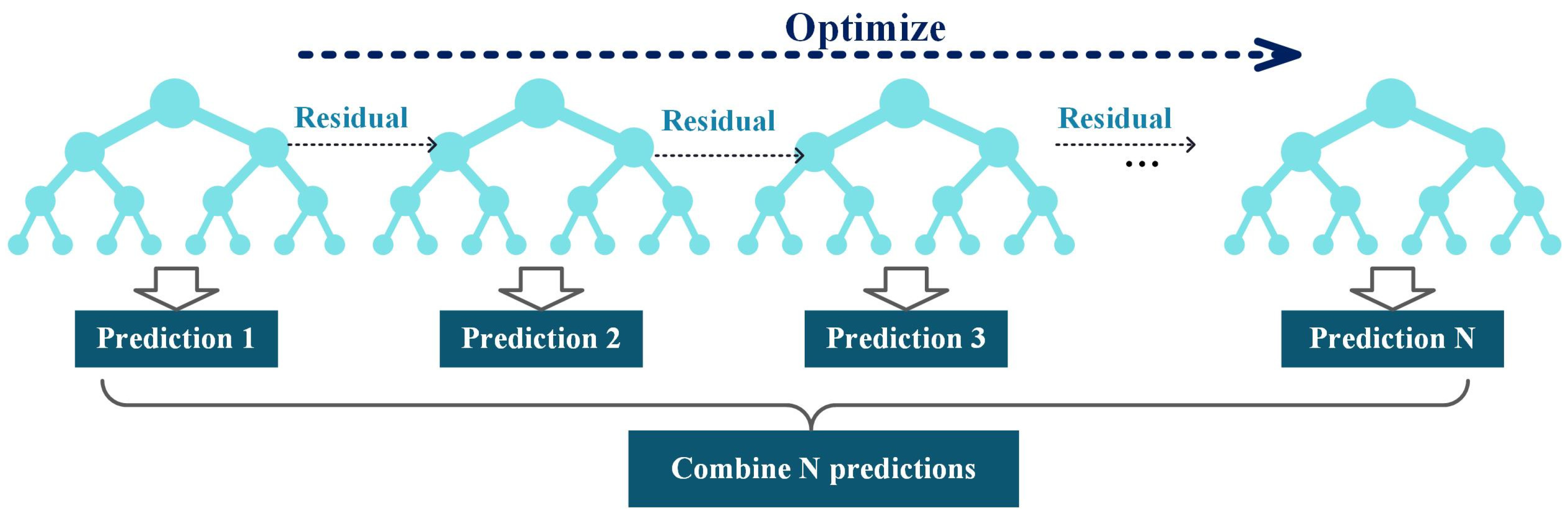
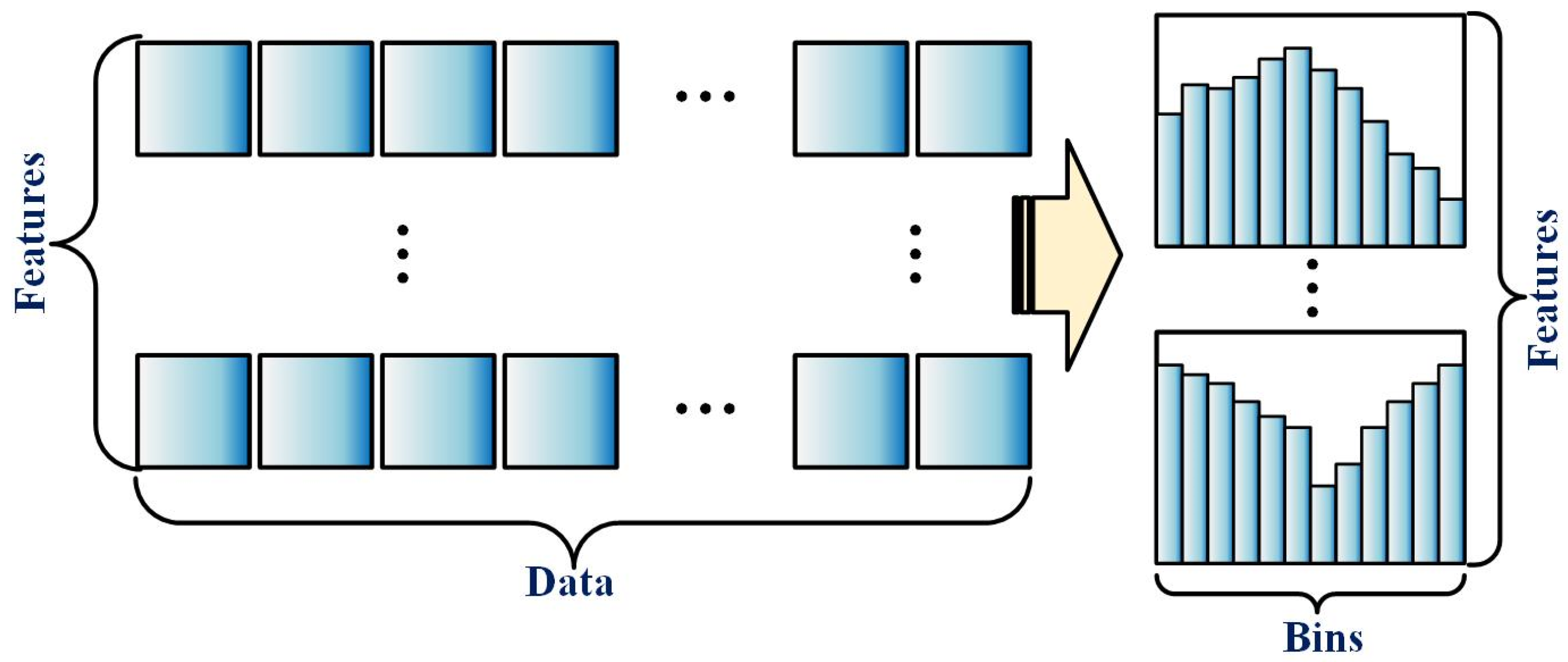
2.1. Histogram Gradient Boosting Tree

Boosting is a strategy to combine multiple weak models to generate a strong model. HGBT belongs to the boosting model, and it is the development of gradient boosting trees (GBT). GBT uses the negative gradient value of the loss function of the current model as an approximation of the residual to fit the classification and regression trees (CART) [55]. The CART generated by each iteration is linearly combined through the addition model to obtain the final classifier. The GBT model has high prediction accuracy and strong robustness, and it can flexibly process various types of data and avoid the over-fitting problem to a certain extent. Figure 2 shows the schematic diagram used to build the GBT model.
HGBT employs the histogram-based algorithm to build the GBT model [65]. The histogram-based algorithm first discretizes the continuous values into multiple integers and constructs a histogram. When traversing the data, statistics are accumulated in the histogram based on the discretized values as indexes. After traversing the data once, the histogram accumulates the required statistics and then traverses to find the optimal segmentation point according to the discrete value of the histogram. Figure 3 shows the schematic diagram of the histogram-based algorithm. The HGBT has a faster computation speed compared to the traditional GBT model. The HGBT model is suitable for incomplete datasets. The HGBT model learns from the data that the sample has missing values during training and thus divides the sample with missing values in accordance with the potential gain at the split point. For inference, the sample with missing values is divided based on the learned rules.

2.2. Hunger Games Search

Hunger game search (HGS) algorithm is introduced to optimize the hyperparameters of the HGBT. HGS [66] was proposed based on starvation-driven activity and the behavior of animals. Animals rely on their sensory knowledge to survive under specific rules and interact with the environment. Animal survival, reproduction, and food opportunities are provided by their numerical logic rules. Hunger is the most important factor in animal life because it directly affects the body balance, behavior, decision, and action. Therefore, animals constantly seek food to maintain this balance and alternate between exploration, defense, and competition activities according to needs. The mathematical model of HGS is as follows
(1)
Approach food
Social animals often cooperate with each other in foraging, but a few individuals might not participate in cooperation. Equation (1) depicts the individual cooperative communication and foraging behavior.
A ( s + 1 ) = Game 1 : A ( s ) ( 1 + r a n d n ( 1 ) ) , a 1 < l Game 2 : M 1 A b + R M 2 A b A ( s ) , a 1 > l , a 2 > E   Game 3 : M 1 A b R M 2 A b A ( s ) , a 1 > l , a 2 < E
E = s e c h ( | F ( i ) B F | )
s e c h ( x ) = 2 e x + e x
where R r a n d [ c , c ] , r a n d ( 1 ) depicts a random value obeying Gaussian distribution, M 1 and M 2 stand for weight of hunger, A b is the location of the optimal individual, A ( s ) is the location of every individual, F ( i ) depicts the fitness of the individual, and B F is the current optimal fitness.
(2)
Hunger role
At this stage, the hunger characteristics of the individual in the search are mathematically simulated by Equation (1). Equations (4) and (5) show the formulas to calculate M 1 and M 2 .
M 1 ( l ) =   hungry ( i ) N   SHungry × a 4 , a 3 < l 1 , a 3 > l
M 2 ( l ) = ( 1 exp ( hungry ( i ) SHungry ) ) × a 5 × 2
where hungry represents the hunger value of each individual, N represents the number of individuals, SHungry represents the sum of all individual hunger, and a 3 , a 4 , a 5 [ 0 , 1 ] .

3. Database

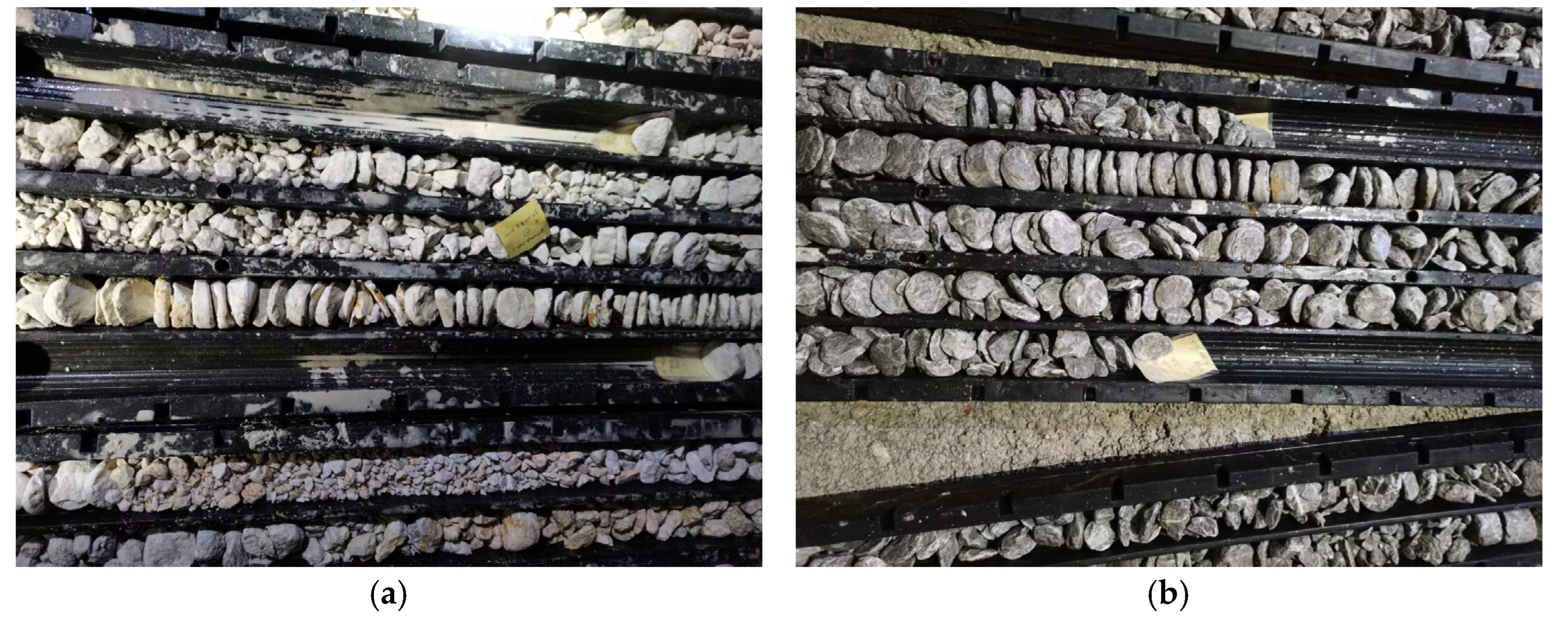
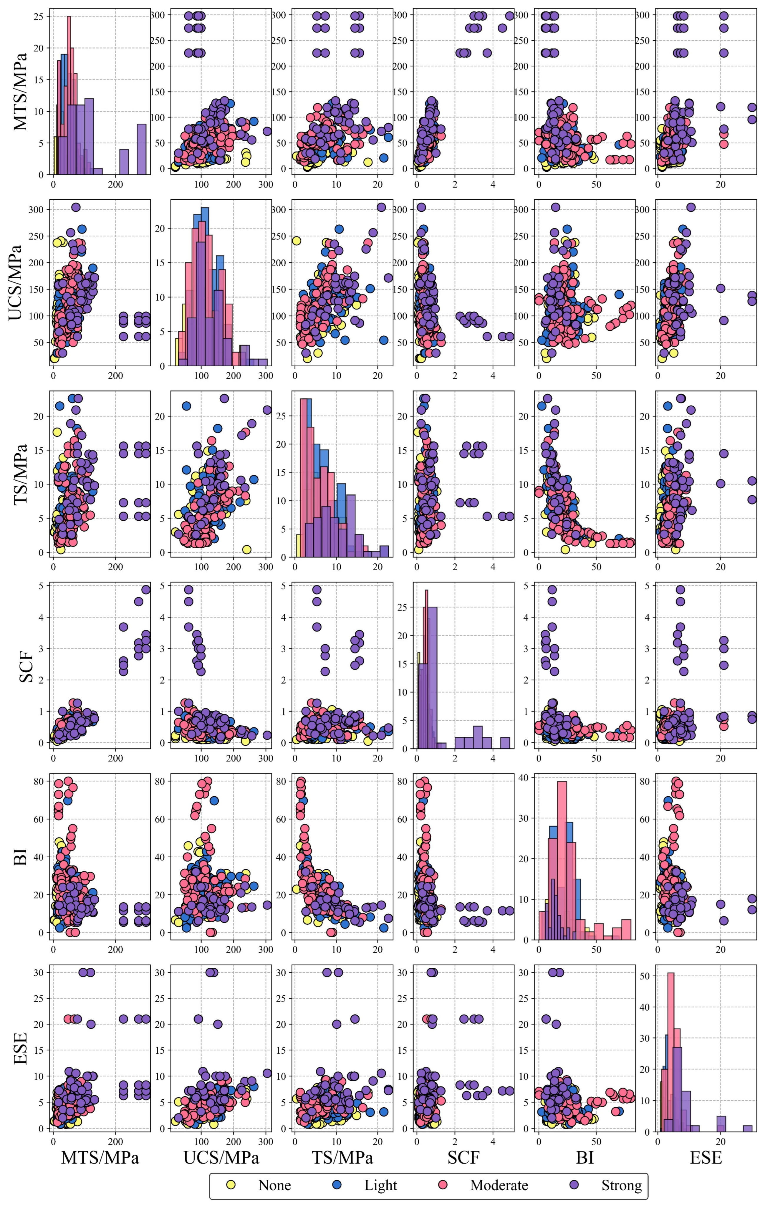
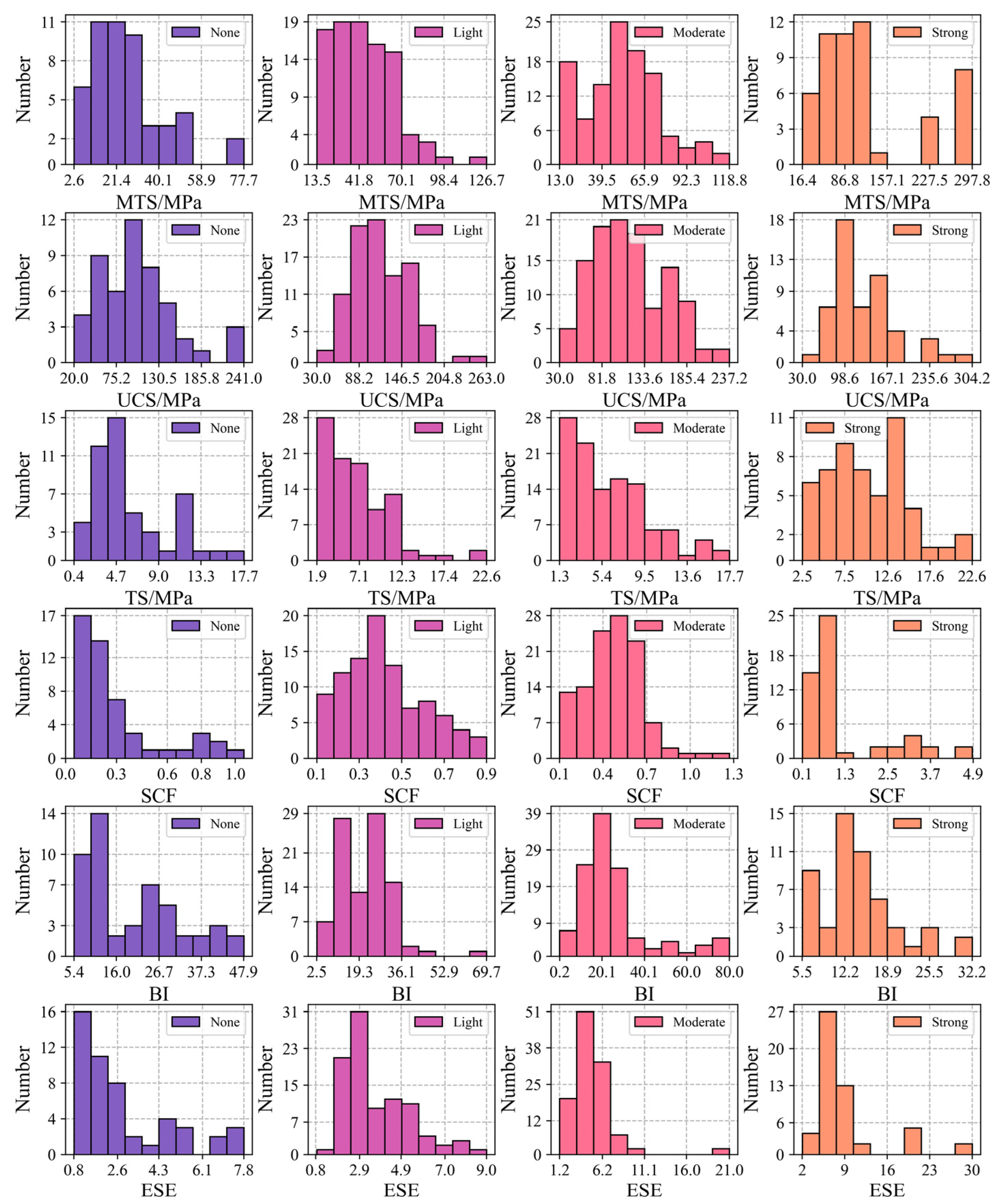
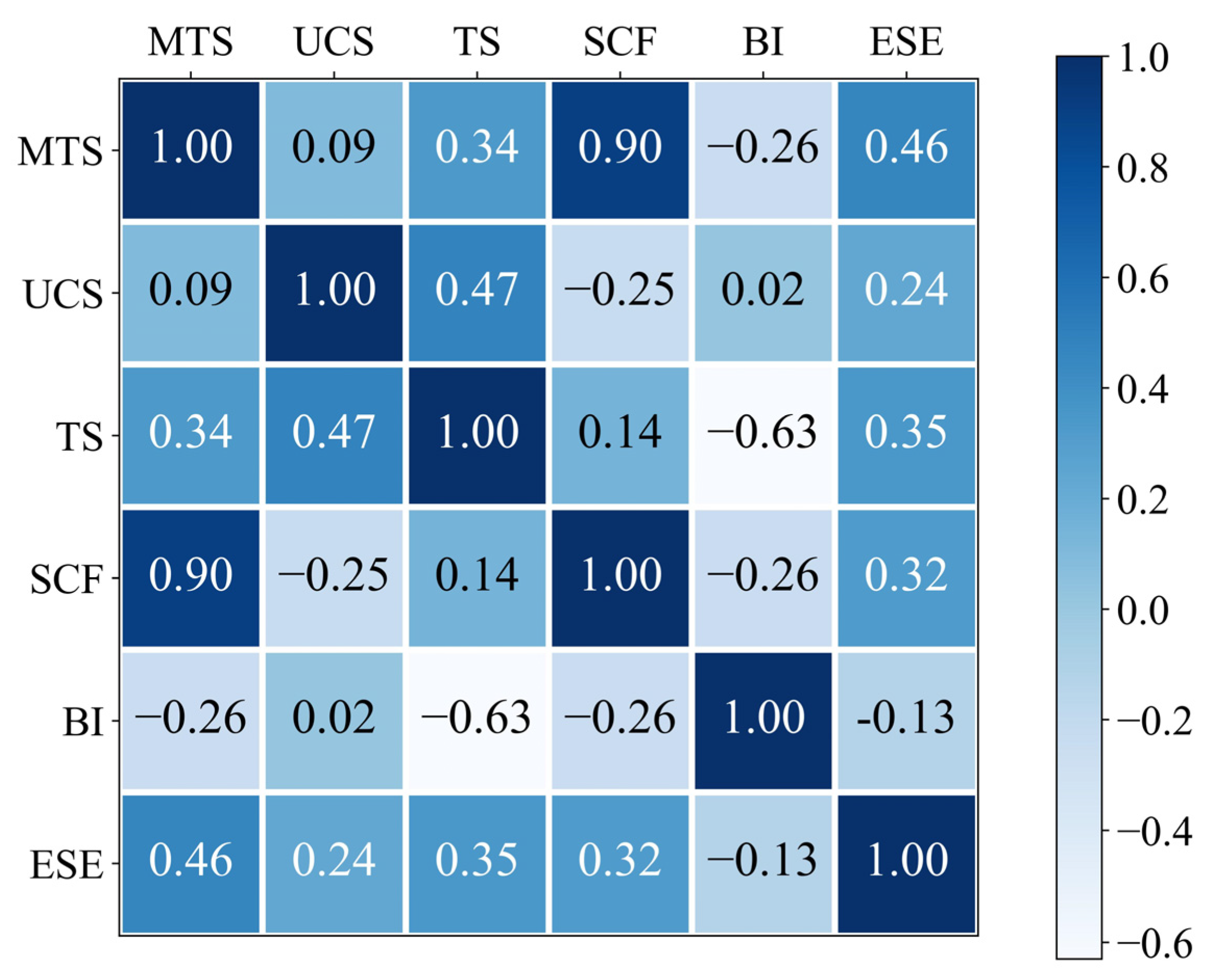
3.1. Data Collection and Description

This study applied the database collected by Li et al. [50], and there were 314 rockburst cases in the database. According to Russenes criteria [67], the intensity levels of rockburst can be classified into none (50 datasets), light (96 datasets), moderate (115 datasets), and strong (53 datasets). Maximum tangential stress (MTS), UCS, tensile strength (TS), stress concentration factor (SCF, i.e., MTS/UCS), brittleness index (BI, i.e., UCS/TS), and elastic strain energy (ESE) were chosen as input variables to develop intelligent models. MTS depicts the strata stress characteristic of rockburst. UCS and TS are the main characteristics of intact rock that impact rockburst. ESE is a measure of the rock’s ability to store elastic energy. SCF and BI are experiential criteria used to evaluate rockburst [6]. These six variables can describe rockburst from different perspectives [6]. Figure 4 shows the scatter distribution of datasets with four intensity levels of rockburst. The range of each variable is shown, and the relationship between any two variables is presented. The distribution of strong rockburst is obviously different from others. Moreover, there are some outliers in the database. These outliers are not processed because the source of the outliers is unknown. Figure 5 shows the histogram distribution of the database. The correlation among the six parameters is calculated, as shown in Figure 6. It can be found that MTS has a strong positive correlation with SCF, and BI has a strong negative correlation with TS. The correlation between other variables is weak.

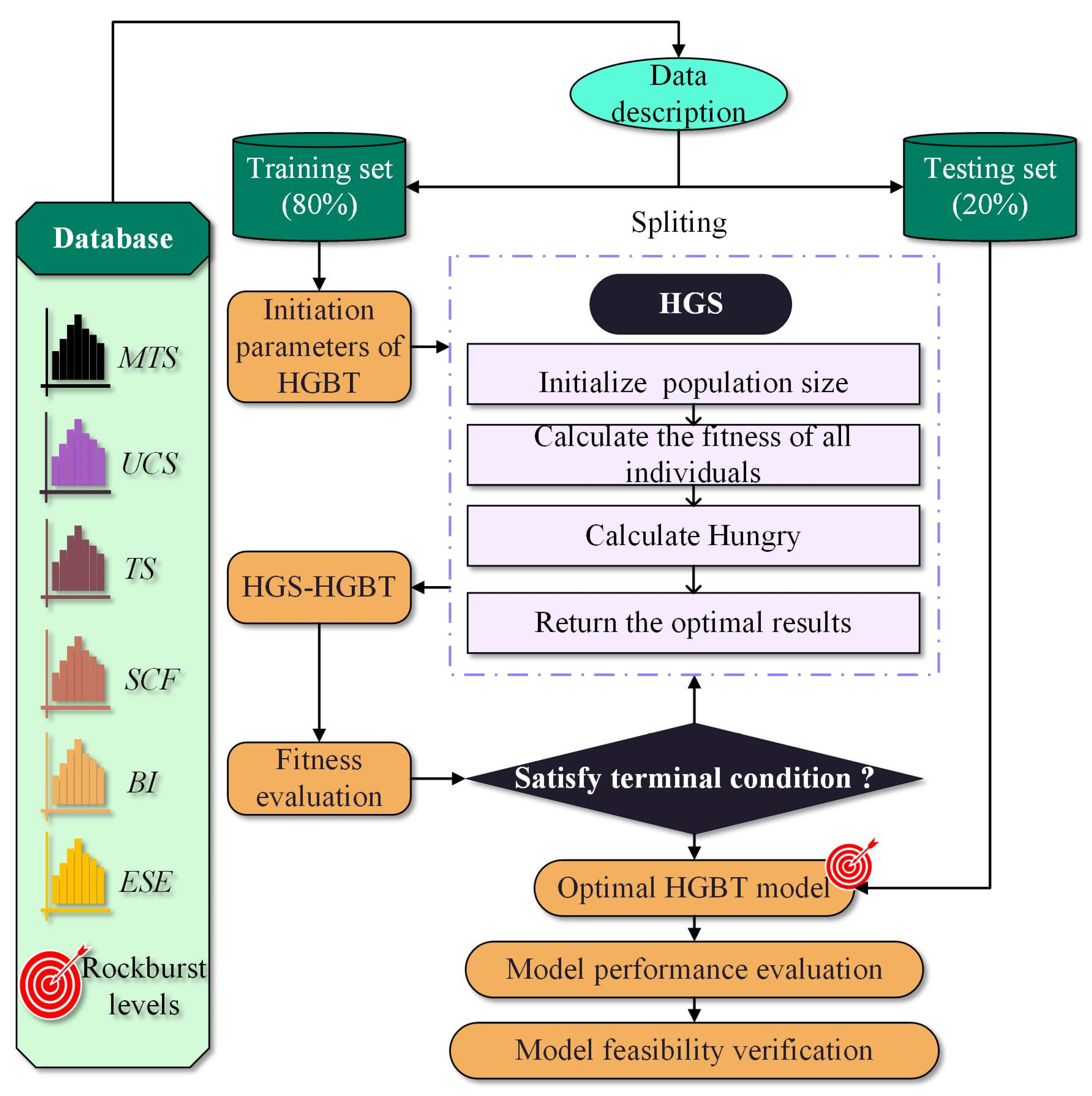
3.2. Step-by-Step Study Flowchart
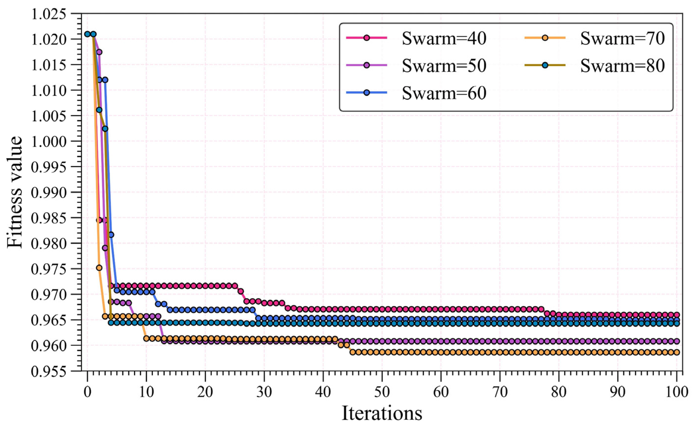
In this study, HGBT and HGS are implemented to build ensemble models suitable for incomplete datasets for rockburst prediction. According to Figure 7, the database is randomly divided into training (80%) and testing (20%) parts. The training datasets are applied to develop the HGBT model. The HGS algorithm is employed to optimize the hyperparameters of the HGBT. The optimal HGBT model is obtained when the termination condition is satisfied. The testing datasets are used to assess the capability of the HGBT model. Finally, rockburst cases from the engineering field are employed to validate the feasibility of the developed HGBT model.

4. Modeling

MTS, UCS, TS, SCF, BI, and ESE in training datasets were normalized (Equation (6)) and input to the HGBT model. Python library, Scikit-learn [68], was applied to develop the histogram gradient boosting tree (HGBT) model. HGS was applied to optimize the parameters of the HGBT model for predicting rockburst intensity levels. The number of swarms affected the performance of models and running time. Population sizes were set to 40, 50, 60, 70, and 80 when optimization techniques were performed. The computation time was 3252.18 s (the CPU was Intel(R) Core(TM) i7-10875H). Figure 8 shows the fitness variation with the increase of iterations. Accuracy (ACC), Kappa, and Matthews correlation coefficient (MCC) were applied to evaluate the performances of developed models. The three classification indicators can be calculated according to Figure 9. When accuracy, Kappa, and MCC were closer to 1, the developed models had more excellent performance.
V = V V ¯ σ
where V ¯ represents the mean value and σ stands for the standard deviation.
Table 1 lists the ACC, Kappa, and MCC of the developed models in the training and testing sets. Rank systems are introduced to compare the optimized HGBT models with different swarm sizes. Training and test performances are ranked separately. HGS-HGBT models with different swarm sizes are ranked according to their performances in each classification indicator, and better performance is associated with a high rank. The ranks of three classification indicators are summed to get the total rank. Table 1 presents the rank systems of these hybrid models. The HGS-HGBT models with different swarm sizes have the same training performances. The HGS-HGBT model with swarm sizes of 80 is the best in terms of testing capacity. To consider the training and testing performances, the total ranks in training and testing sets are summed to obtain the final rank. The final rank is applied to select models, and a higher final rank is accompanied by a better comprehensive performance. Figure 10 displays the final rank of the five hybrid models. The HGS-HGBT model with swarm sizes of 80 is the optimal model according to the final rank. It receives an accuracy of 0.89, Kappa of 0.84, and MCC of 0.85 in testing datasets.

5. Discussion

5.1. Performance Evaluation of HGBT in Incomplete Datasets

The HGBT model was developed and chosen based on the collected database. To analyze the superiority of HGBT, an additional database with missing values was collected. The database with missing values was from Afraei et al. [9]. Table 2 presents the database. These datasets with missing values were input into the HGBT model, and the accuracy was computed. Additionally, these missing values were filled by 0 and the mean, median, and most frequent values of training datasets. RF, gradient boosting machine (GBM), adaptive gradient boosting (AdaBoost), XGBoost, SVM, ANN, and KNN were also developed by training datasets. The incomplete database was completed by four different methods and then was applied to evaluate these models. Figure 11 exhibits the accuracy of HGBT and other models in completed databases by four different methods. HGBT received an accuracy of 77.78% in the incomplete database. In the other seven models, AdaBoost and KNN had the best performance in the databases filled with 0 and the most frequent value, and ANN had the optimal capability in databases filled with the mean value and median value. HGBT had higher accuracy than AdaBoost, KNN, and ANN. The results suggested that HGBT had a huge advantage in rockburst prediction with incomplete datasets. The developed HGBT was more suitable for field application, considering the cost and difficulty of measuring datasets.

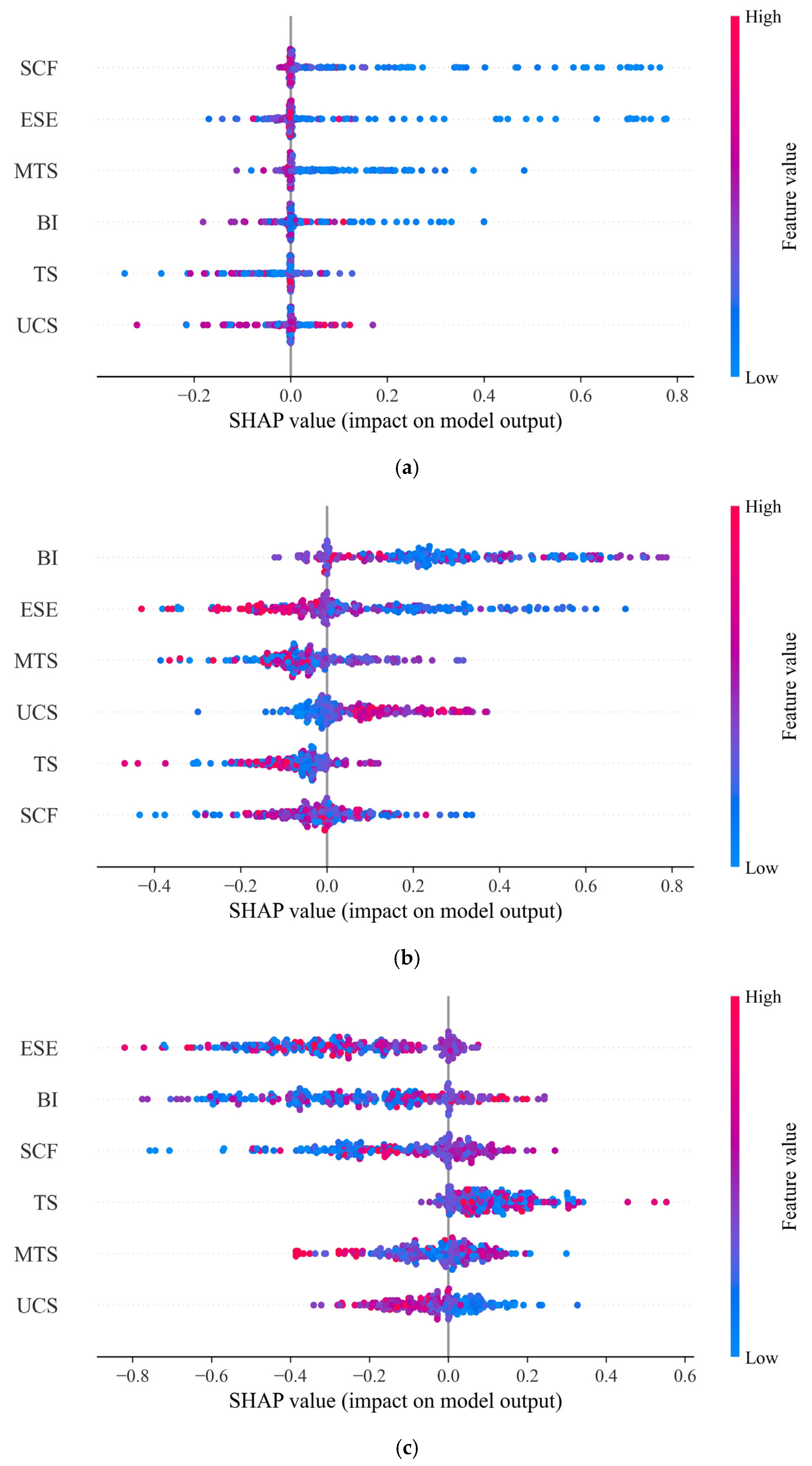
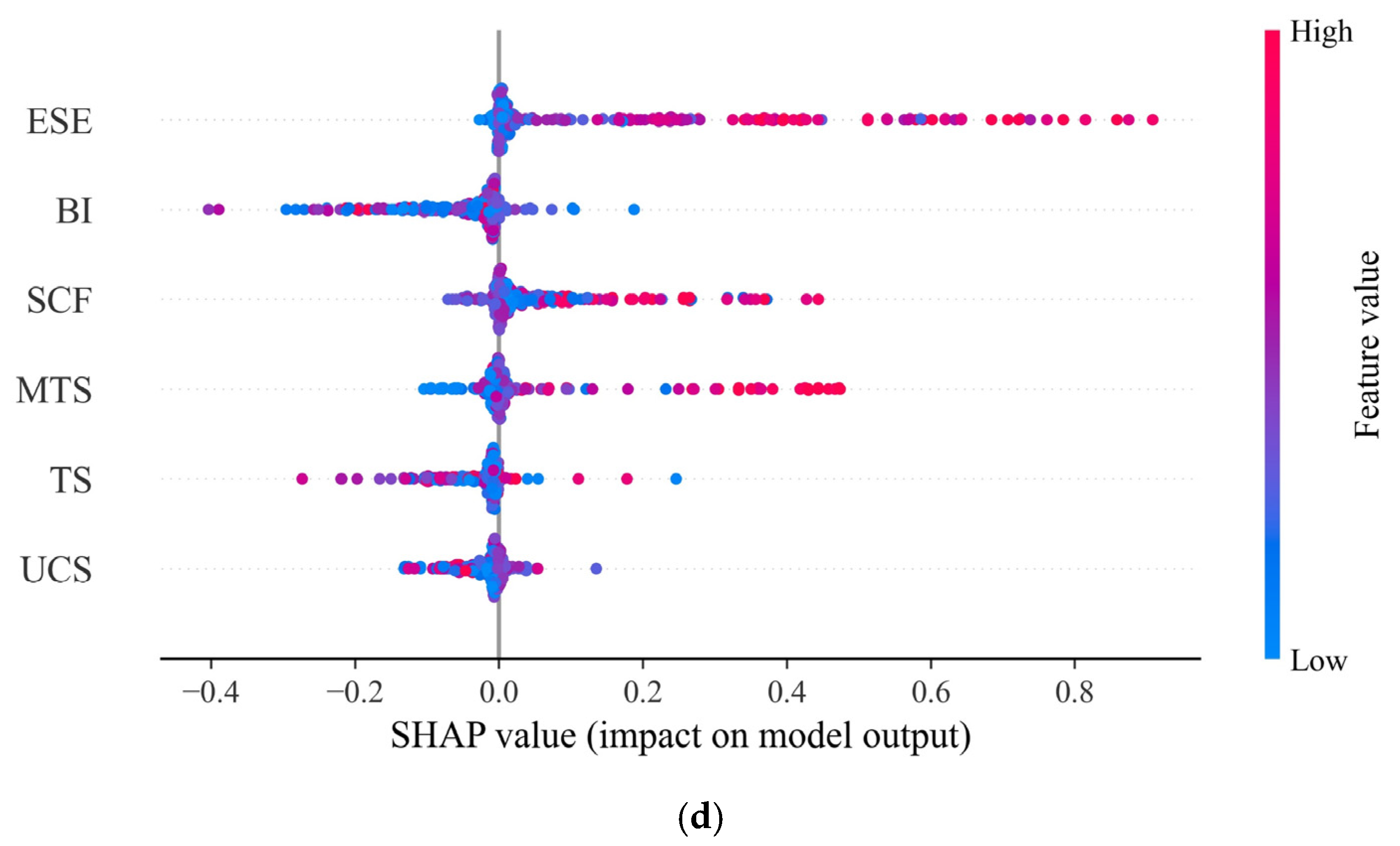
5.2. Model Interpretation

The rockburst mechanism was very complex, and the rockburst events were related to multiple factors. This study considered six factors to evaluate rockburst intensity levels. The analysis of essential factors and their influence on rockburst grades was conducive to predicting and preventing rockburst. To determine the influence of the input parameters, Shapley additive explanation (SHAP) was introduced to explain the established HGBT model. SHAP was mainly used to account for the predicted process of an individual, and it was developed according to the optimal Shapley in game theory [69]. In SHAP, the predicted process of a sample was derived by calculating the contribution of each feature to the predicted result. Shapley value was calculated, and it depicted the average division of prediction between features. A detailed introduction to SHAP can be found in Lundberg and Lee [69].
The importance of variables can be obtained by SHAP, and the variable with the larger absolute value of Shapley is more important. Figure 12 presents an overview diagram of SHAP to explain the HGBT in rockburst evaluation with different intensity levels. The overview diagram of SHAP combines the importance of parameters and their impact on rockburst intensity levels. In the figure, the vertical axis exhibits the six input variables, and the horizontal axis stands for the Shapley value. Each point depicts a sample and the Shapley value of the sample. The color variations of points from blue to red represent the value variations of variables from low to high. The overlapping points vibrate on the ordinate, and the variables are sorted from top to bottom according to their importance. According to this law, SCF and BI are essential for the prediction of none and light rockbursts, respectively. ESE is crucial for the prediction of four types of rockburst, especially for moderate and strong rockburst. The results are consistent with previous studies [47,50,52,53,60,61], which suggests that the developed HGBT model was reasonable. Moreover, it is noted that the occurrence of strong rockburst is associated with large ESE. Some measures to reduce ESE can be applied to alleviate rockburst, such as borehole pressure relief, smooth blasting, and energy-absorbing anchors.

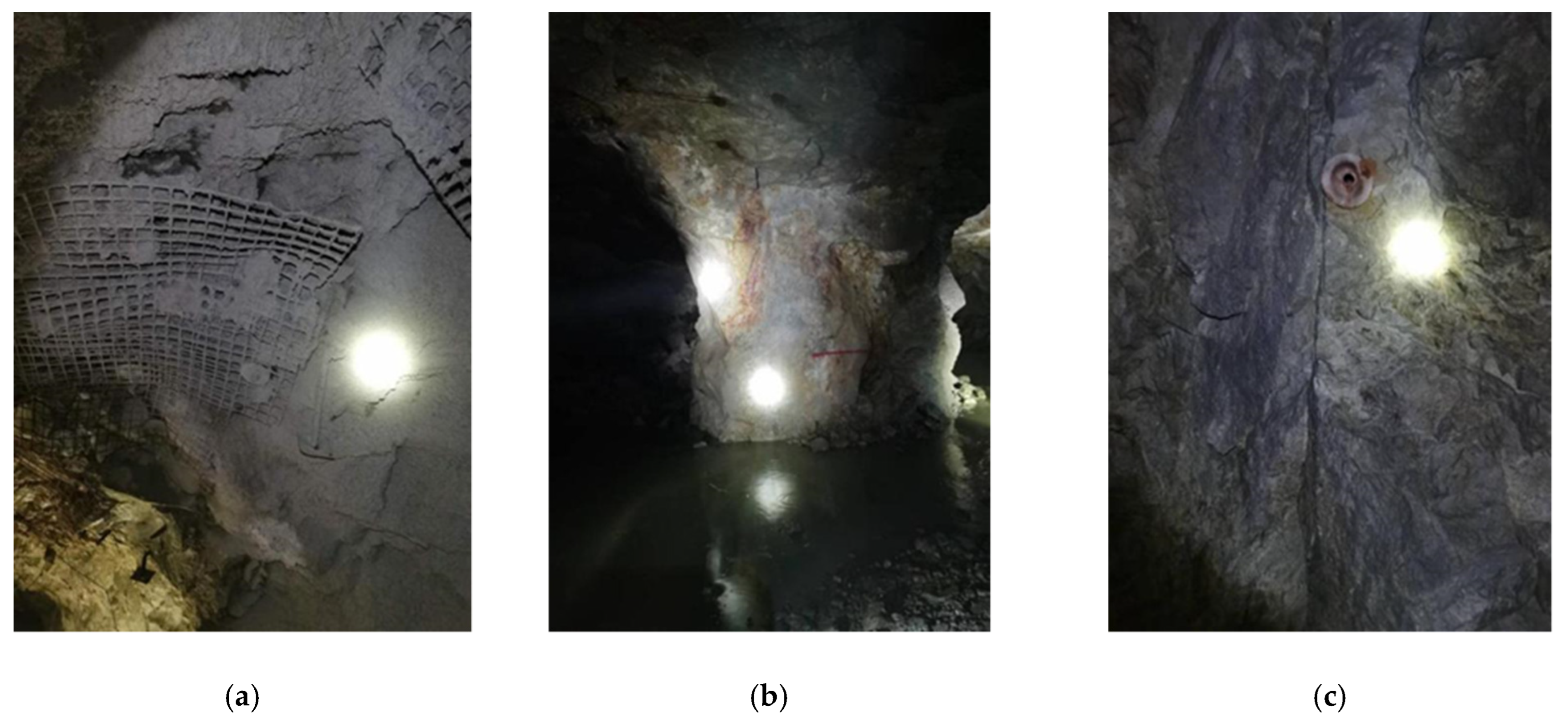
5.3. Model Feasibility Verification

To validate the model feasibility, the developed HGBT model was implemented to evaluate the rockburst in Sanshandao Gold Mine, Shandong, China. Sanshandao Gold Mine is a typical submarine-mining metal mine. As one of the largest gold mines in China, Sanshandao Gold Mine has reached a mining depth of more than kilometers. The depth of proven exploitable resources in Sanshandao Gold Mine is below 1500 m, and the exploitable depth is 1225 m. Deep mining is faced with a harsh environment of high temperature, high ground pressure, and high seepage, which is obviously different from shallow mining. Due to the influence of high ground pressure, rockburst becomes a major factor limiting deep mining in Sanshandao Gold Mine. The rockburst propensity of rock masses at depths below 700 m is high, and rockburst events with different intensity levels have been reported in Sanshandao Gold Mine. The typical rockburst disasters of Sanshandao Gold Mine are shown in Figure 13. To prevent rockburst and ensure production safety, site investigations and rock tests were conducted. Nine datasets, including MTS, UCS, TS, SCF, BI, and ESE, were measured, and the rockburst intensity levels were determined according to failure conditions in the field and Russenes criteria. Table 3 compiles these measured rockburst datasets. HGBT received an accuracy of 100% in these datasets. The results indicated that the developed HGBT had satisfactory engineering practicability.

6. Conclusions

The HGBT model, an ensemble model based on decision trees, was implemented to build intelligent models for rockburst prediction. An incomplete database was applied to validate the application of HGBT in datasets with missing values. HGBT had a higher accuracy compared to the combination of other models and strategies of completing missing values. The results suggested that the developed HGBT model had a significant advantage in incomplete datasets, which was more suitable for application in engineering sites. Moreover, SHAP was introduced to interpret the developed HGBT model. The key parameters affecting different rockburst grades were determined. ESE was the crucial variable for the prediction of moderate and strong rockburst. The happening of strong rockburst was associated with large ESE. Finally, real rockburst cases were collected in Sanshandao Gold Mine, China. These datasets were applied to verify the feasibility of the developed HGBT model. The evaluated results of the HGBT model matched the real rockburst events on site, which demonstrated the great feasibility of the HGBT model.
Six factors reflecting the characteristics of strata stress and rock properties were considered to evaluate rockburst in this study. However, some other factors, such as rock mass structure, blasting disturbance, and excavation method, also had an influence on rockburst. In the future, considering more related variables is beneficial to predict rockburst efficiently and precisely. Additionally, collecting more rockburst cases to increase the database size can improve the robustness of intelligent models.

Author Contributions

Conceptualization, H.L. and G.Z.; methodology, H.L.; software, H.L.; validation, P.X.; investigation, P.X.; writing—original draft preparation, H.L.; writing—review and editing, P.X., G.Z. and Y.Y.; visualization, H.L. All authors have read and agreed to the published version of the manuscript.

Funding

This research received no external funding.

Data Availability Statement

The data presented in this study are available on request from the corresponding author.

Conflicts of Interest

The authors declare no conflict of interest.

References

  1. Keneti, A.; Sainsbury, B.-A. Review of published rockburst events and their contributing factors. Eng. Geol. 2018, 246, 361–373. [Google Scholar] [CrossRef]
  2. Skrzypkowski, K. A new design of support for burst-prone rock mass in underground ore mining. E3S Web Conf. 2018, 71, 00006. [Google Scholar] [CrossRef]
  3. Shirani Faradonbeh, R.; Taheri, A.; Karakus, M. The propensity of the over-stressed rock masses to different failure mechanisms based on a hybrid probabilistic approach. Tunn. Undergr. Space Technol. 2022, 119, 104214. [Google Scholar] [CrossRef]
  4. Wang, J.-A.; Park, H. Comprehensive prediction of rockburst based on analysis of strain energy in rocks. Tunn. Undergr. Space Technol. 2001, 16, 49–57. [Google Scholar] [CrossRef]
  5. Chen, B.-R.; Feng, X.-T.; Li, Q.-P.; Luo, R.-Z.; Li, S. Rock Burst Intensity Classification Based on the Radiated Energy with Damage Intensity at Jinping II Hydropower Station, China. Rock Mech. Rock Eng. 2015, 48, 289–303. [Google Scholar] [CrossRef]
  6. Zhou, J.; Li, X.; Shi, X. Long-term prediction model of rockburst in underground openings using heuristic algorithms and support vector machines. Saf. Sci. 2012, 50, 629–644. [Google Scholar] [CrossRef]
  7. Lee, S.M.; Park, B.S.; Lee, S.W. Analysis of rockbursts that have occurred in a waterway tunnel in Korea. Int. J. Rock Mech. Min. Sci. 2004, 41, 911–916. [Google Scholar] [CrossRef]
  8. Manouchehrian, A.; Cai, M. Numerical modeling of rockburst near fault zones in deep tunnels. Tunn. Undergr. Space Technol. 2018, 80, 164–180. [Google Scholar] [CrossRef]
  9. Afraei, S.; Shahriar, K.; Madani, S.H. Developing intelligent classification models for rock burst prediction after recognizing significant predictor variables, Section 1: Literature review and data preprocessing procedure. Tunn. Undergr. Space Technol. 2019, 83, 324–353. [Google Scholar] [CrossRef]
  10. Afraei, S.; Shahriar, K.; Madani, S.H. Developing intelligent classification models for rock burst prediction after recognizing significant predictor variables, Section 2: Designing classifiers. Tunn. Undergr. Space Technol. 2019, 84, 522–537. [Google Scholar] [CrossRef]
  11. Shirani Faradonbeh, R.; Taheri, A.; Ribeiro e Sousa, L.; Karakus, M. Rockburst assessment in deep geotechnical conditions using true-triaxial tests and data-driven approaches. Int. J. Rock Mech. Min. Sci. 2020, 128, 104279. [Google Scholar] [CrossRef]
  12. Dowding, C.H.; Andersson, C.-A. Potential for rock bursting and slabbing in deep caverns. Eng. Geol. 1986, 22, 265–279. [Google Scholar] [CrossRef]
  13. Pu, Y.; Apel, D.B.; Liu, V.; Mitri, H. Machine learning methods for rockburst prediction-state-of-the-art review. Int. J. Min. Sci. Technol. 2019, 29, 565–570. [Google Scholar] [CrossRef]
  14. Shirani Faradonbeh, R.; Taheri, A. Long-term prediction of rockburst hazard in deep underground openings using three robust data mining techniques. Eng. Comput. 2018, 35, 659–675. [Google Scholar] [CrossRef]
  15. Liang, W.; Zhao, G. A review of long-term and short-term rockburst risk evaluations in deep hard rock. Yanshilixue Yu Gongcheng Xuebao/Chin. J. Rock Mech. Eng. 2022, 41, 19–39. [Google Scholar] [CrossRef]
  16. Liang, W.; Sari, Y.A.; Zhao, G.; McKinnon, S.D.; Wu, H. Probability Estimates of Short-Term Rockburst Risk with Ensemble Classifiers. Rock Mech. Rock Eng. 2021, 54, 1799–1814. [Google Scholar] [CrossRef]
  17. Ullah, B.; Kamran, M.; Rui, Y. Predictive Modeling of Short-Term Rockburst for the Stability of Subsurface Structures Using Machine Learning Approaches: T-SNE, K-Means Clustering and XGBoost. Mathematics 2022, 10, 449. [Google Scholar] [CrossRef]
  18. He, M.; Cheng, T.; Qiao, Y.; Li, H. A review of rockburst: Experiments, theories, and simulations. J. Rock Mech. Geotech. Eng. 2022. [Google Scholar] [CrossRef]
  19. Kabwe, E.; Wang, Y. Review on Rockburst Theory and Types of Rock Support in Rockburst Prone Mines. Open J. Saf. Sci. Technol. 2015, 5, 18. [Google Scholar] [CrossRef] [Green Version]
  20. Askaripour, M.; Saeidi, A.; Rouleau, A.; Mercier-Langevin, P. Rockburst in underground excavations: A review of mechanism, classification, and prediction methods. Undergr. Space 2022, 7, 577–607. [Google Scholar] [CrossRef]
  21. Zhou, J.; Li, X.; Mitri, H.S. Evaluation method of rockburst: State-of-the-art literature review. Tunn. Undergr. Space Technol. 2018, 81, 632–659. [Google Scholar] [CrossRef]
  22. Xiao, P.; Li, D.; Zhao, G.; Liu, M. Experimental and Numerical Analysis of Mode I Fracture Process of Rock by Semi-Circular Bend Specimen. Mathematics 2021, 9, 1769. [Google Scholar] [CrossRef]
  23. Zhou, X.; Zhang, G.; Song, Y.; Hu, S.; Liu, M.; Li, J. Evaluation of rock burst intensity based on annular grey target decision-making model with variable weight. Arab. J. Geosci. 2019, 12, 43. [Google Scholar] [CrossRef]
  24. Xue, Y.; Li, Z.; Li, S.; Qiu, D.; Tao, Y.; Wang, L.; Yang, W.; Zhang, K. Prediction of rock burst in underground caverns based on rough set and extensible comprehensive evaluation. Bull. Eng. Geol. Environ. 2019, 78, 417–429. [Google Scholar] [CrossRef]
  25. Liang, W.; Zhao, G.; Wu, H.; Dai, B. Risk assessment of rockburst via an extended MABAC method under fuzzy environment. Tunn. Undergr. Space Technol. 2019, 83, 533–544. [Google Scholar] [CrossRef]
  26. Xue, Y.; Bai, C.; Kong, F.; Qiu, D.; Li, L.; Su, M.; Zhao, Y. A two-step comprehensive evaluation model for rockburst prediction based on multiple empirical criteria. Eng. Geol. 2020, 268, 105515. [Google Scholar] [CrossRef]
  27. Xue, Y.; Bai, C.; Qiu, D.; Kong, F.; Li, Z. Predicting rockburst with database using particle swarm optimization and extreme learning machine. Tunn. Undergr. Space Technol. 2020, 98, 103287. [Google Scholar] [CrossRef]
  28. Zhou, J.; Koopialipoor, M.; Li, E.; Armaghani, D.J. Prediction of rockburst risk in underground projects developing a neuro-bee intelligent system. Bull. Eng. Geol. Environ. 2020, 79, 4265–4279. [Google Scholar] [CrossRef]
  29. Ribeiro e Sousa, L.; Miranda, T.; Leal e Sousa, R.; Tinoco, J. The Use of Data Mining Techniques in Rockburst Risk Assessment. Engineering 2017, 3, 552–558. [Google Scholar] [CrossRef]
  30. Wang, J.; Apel, D.B.; Pu, Y.; Hall, R.; Wei, C.; Sepehri, M. Numerical modeling for rockbursts: A state-of-the-art review. J. Rock Mech. Geotech. Eng. 2021, 13, 457–478. [Google Scholar] [CrossRef]
  31. Zubelewicz, A.; Mróz, Z. Numerical simulation of rock burst processes treated as problems of dynamic instability. Rock Mech. Rock Eng. 1983, 16, 253–274. [Google Scholar] [CrossRef]
  32. Wang, S.Y.; Lam, K.C.; Au, S.K.; Tang, C.A.; Zhu, W.C.; Yang, T.H. Analytical and Numerical Study on the Pillar Rockbursts Mechanism. Rock Mech. Rock Eng. 2006, 39, 445–467. [Google Scholar] [CrossRef]
  33. Pu, Y.; Apel, D.B.; Wei, C. Applying Machine Learning Approaches to Evaluating Rockburst Liability: A Comparation of Generative and Discriminative Models. Pure Appl. Geophys. 2019, 176, 4503–4517. [Google Scholar] [CrossRef]
  34. Pu, Y.; Apel, D.B.; Wang, C.; Wilson, B. Evaluation of burst liability in kimberlite using support vector machine. Acta Geophys. 2018, 66, 973–982. [Google Scholar] [CrossRef]
  35. Pu, Y.; Apel, D.B.; Lingga, B. Rockburst prediction in kimberlite using decision tree with incomplete data. J. Sustain. Min. 2018, 17, 158–165. [Google Scholar] [CrossRef]
  36. Liu, Z.; Armaghani, D.-J.; Fakharian, P.; Li, D.; Ulrikh, D.-V.; Orekhova, N.-N.; Khedher, K.-M. Rock Strength Estimation Using Several Tree-Based ML Techniques. Comput. Model. Eng. Sci. 2022, 133, 799–824. [Google Scholar] [CrossRef]
  37. Li, G.; Xue, Y.; Qu, C.; Qiu, D.; Wang, P.; Liu, Q. Intelligent prediction of rockburst in tunnels based on back propagation neural network integrated beetle antennae search algorithm. Environ. Sci. Pollut. Res. 2022. [Google Scholar] [CrossRef]
  38. Kadkhodaei, M.H.; Ghasemi, E. Development of a Semi-quantitative Framework to Assess Rockburst Risk Using Risk Matrix and Logistic Model Tree. Geotech. Geol. Eng. 2022, 40, 3669–3685. [Google Scholar] [CrossRef]
  39. Kadkhodaei, M.H.; Ghasemi, E.; Sari, M. Stochastic assessment of rockburst potential in underground spaces using Monte Carlo simulation. Environ. Earth Sci. 2022, 81, 447. [Google Scholar] [CrossRef]
  40. Wang, H.; Li, Z.; Song, D.; He, X.; Sobolev, A.; Khan, M. An Intelligent Rockburst Prediction Model Based on Scorecard Methodology. Minerals 2021, 11, 1294. [Google Scholar] [CrossRef]
  41. Ghasemi, E.; Gholizadeh, H.; Adoko, A.C. Evaluation of rockburst occurrence and intensity in underground structures using decision tree approach. Eng. Comput. 2019, 36, 213–225. [Google Scholar] [CrossRef]
  42. Shaidurov, G.Y.; Kudinov, D.S.; Kokhonkova, E.A. On the possibility of creating a comprehensive system for rockburst prediction in mines and mining plants. J. Phys. Conf. Ser. 2019, 1399, 033100. [Google Scholar] [CrossRef]
  43. Shirani Faradonbeh, R.; Shaffiee Haghshenas, S.; Taheri, A.; Mikaeil, R. Application of self-organizing map and fuzzy c-mean techniques for rockburst clustering in deep underground projects. Neural Comput. Appl. 2020, 32, 8545–8559. [Google Scholar] [CrossRef]
  44. Zhou, J.; Shi, X.-z.; Dong, L.; Hu, H.-y.; Wang, H.-y. Fisher discriminant analysis model and its application for prediction of classification of rockburst in deep-buried long tunnel. J. Coal Sci. Eng. 2010, 16, 144–149. [Google Scholar] [CrossRef]
  45. Li, N.; Jimenez, R. A logistic regression classifier for long-term probabilistic prediction of rock burst hazard. Nat. Hazards 2018, 90, 197–215. [Google Scholar] [CrossRef]
  46. Zhou, J.; Li, X.; Mitri, H.S. Classification of Rockburst in Underground Projects: Comparison of Ten Supervised Learning Methods. J. Comput. Civ. Eng. 2016, 30, 04016003. [Google Scholar] [CrossRef]
  47. Zhou, J.; Guo, H.; Koopialipoor, M.; Jahed Armaghani, D.; Tahir, M.M. Investigating the effective parameters on the risk levels of rockburst phenomena by developing a hybrid heuristic algorithm. Eng. Comput. 2020, 37, 1679–1694. [Google Scholar] [CrossRef]
  48. Zhang, M. Prediction of rockburst hazard based on particle swarm algorithm and neural network. Neural Comput. Appl. 2021, 34, 2649–2659. [Google Scholar] [CrossRef]
  49. Zhang, G.; Gao, Q.; Du, J.; Li, K. Rockburst criterion based on artificial neural networks and nonlinear regression. J. Cent. South Univ. 2013, 44, 2977–2981. [Google Scholar]
  50. Li, D.; Liu, Z.; Xiao, P.; Zhou, J.; Jahed Armaghani, D. Intelligent rockburst prediction model with sample category balance using feedforward neural network and Bayesian optimization. Undergr. Space 2022, 7, 833–846. [Google Scholar] [CrossRef]
  51. Pu, Y.; Apel, D.B.; Xu, H. Rockburst prediction in kimberlite with unsupervised learning method and support vector classifier. Tunn. Undergr. Space Technol. 2019, 90, 12–18. [Google Scholar] [CrossRef]
  52. Xue, Y.; Li, G.; Li, Z.; Wang, P.; Gong, H.; Kong, F. Intelligent prediction of rockburst based on Copula-MC oversampling architecture. Bull. Eng. Geol. Environ. 2022, 81, 209. [Google Scholar] [CrossRef]
  53. Zhang, J.; Wang, Y.; Sun, Y.; Li, G. Strength of ensemble learning in multiclass classification of rockburst intensity. Int. J. Numer. Anal. Methods Geomech. 2020, 44, 1833–1853. [Google Scholar] [CrossRef]
  54. Breiman, L. Random Forests. MLear 2001, 45, 5–32. [Google Scholar] [CrossRef] [Green Version]
  55. Friedman, J.H. Greedy Function Approximation: A Gradient Boosting Machine. Ann. Stat. 2001, 29, 1189–1232. [Google Scholar] [CrossRef]
  56. Geurts, P.; Ernst, D.; Wehenkel, L. Extremely randomized trees. MLear 2006, 63, 3–42. [Google Scholar] [CrossRef] [Green Version]
  57. Yin, X.; Liu, Q.; Pan, Y.; Huang, X.; Wu, J.; Wang, X. Strength of Stacking Technique of Ensemble Learning in Rockburst Prediction with Imbalanced Data: Comparison of Eight Single and Ensemble Models. Nat. Resour. Res. 2021, 30, 1795–1815. [Google Scholar] [CrossRef]
  58. Wang, S.-m.; Zhou, J.; Li, C.-q.; Armaghani, D.J.; Li, X.-b.; Mitri, H.S. Rockburst prediction in hard rock mines developing bagging and boosting tree-based ensemble techniques. J. Cent. South Univ. 2021, 28, 527–542. [Google Scholar] [CrossRef]
  59. Shukla, R.; Khandelwal, M.; Kankar, P.K. Prediction and Assessment of Rock Burst Using Various Meta-heuristic Approaches. Min. Metall. Explor. 2021, 38, 1375–1381. [Google Scholar] [CrossRef]
  60. Li, D.; Liu, Z.; Armaghani, D.J.; Xiao, P.; Zhou, J. Novel ensemble intelligence methodologies for rockburst assessment in complex and variable environments. Sci. Rep. 2022, 12, 1844. [Google Scholar] [CrossRef]
  61. Li, D.; Liu, Z.; Armaghani, D.J.; Xiao, P.; Zhou, J. Novel Ensemble Tree Solution for Rockburst Prediction Using Deep Forest. Mathematics 2022, 10, 787. [Google Scholar] [CrossRef]
  62. Ahmad, M.; Katman, H.Y.; Al-Mansob, R.A.; Ahmad, F.; Safdar, M.; Alguno, A.C. Prediction of Rockburst Intensity Grade in Deep Underground Excavation Using Adaptive Boosting Classifier. Complexity 2022, 2022, 6156210. [Google Scholar] [CrossRef]
  63. Xiao, P.; Li, D.; Zhao, G.; Liu, H. New criterion for the spalling failure of deep rock engineering based on energy release. Int. J. Rock Mech. Min. Sci. 2021, 148, 104943. [Google Scholar] [CrossRef]
  64. Lim, S.S.; Martin, C.D. Core disking and its relationship with stress magnitude for Lac du Bonnet granite. Int. J. Rock Mech. Min. Sci. 2010, 47, 254–264. [Google Scholar] [CrossRef]
  65. Aljamaan, H.; Alazba, A. Software defect prediction using tree-based ensembles. In Proceedings of the 16th ACM International Conference on Predictive Models and Data Analytics in Software Engineering, Virtual Event, 8–9 November 2020; pp. 1–10. [Google Scholar]
  66. Yang, Y.; Chen, H.; Heidari, A.A.; Gandomi, A.H. Hunger games search: Visions, conception, implementation, deep analysis, perspectives, and towards performance shifts. Expert Syst. Appl. 2021, 177, 114864. [Google Scholar] [CrossRef]
  67. Russenes, B. Analysis of rock spalling for tunnels in steep valley sides. Master’s Thesis, Norwegian Institute of Technology, Department of Geology, Trondheim, Norway, 1974. [Google Scholar]
  68. Pedregosa, F.; Varoquaux, G.; Gramfort, A.; Michel, V.; Thirion, B.; Grisel, O.; Blondel, M.; Prettenhofer, P.; Weiss, R.; Dubourg, V. Scikit-learn: Machine learning in Python. the J. Mach. Learn. Res. 2011, 12, 2825–2830. [Google Scholar]
  69. Lundberg, S.M.; Lee, S.-I. A unified approach to interpreting model predictions. In Proceedings of the Advances in Neural Information Processing Systems, Long Beach, CA, USA, 4–9 December 2017; pp. 4768–4777. [Google Scholar]
Figure 1. Core disking in a deep mine in China: (a) Mining depth of 950 m; (b) Mining depth of 1050 m.
Minerals 13 00103 g001
Figure 2. Schematic diagram to build the GBT model.
Minerals 13 00103 g002
Figure 3. Schematic diagram for the histogram-based algorithm.
Minerals 13 00103 g003
Figure 4. The scatter distribution of the database.
Minerals 13 00103 g004
Figure 5. Histogram distribution of the database.
Minerals 13 00103 g005
Figure 6. The correlation of six variables.
Minerals 13 00103 g006
Figure 7. The technique flowchart of this study.
Minerals 13 00103 g007
Figure 8. The fitness variation during the optimization process.
Minerals 13 00103 g008
Figure 9. Schematic diagram to calculate ACC, Kappa, and MCC. Pe depicts expected agreement when both annotators assign labels randomly, t k represents the number of times class k truly occurred, p k is the number of times class k was predicted, c stands for the total number of samples correctly predicted, and s represents the total number of samples.
Minerals 13 00103 g009
Figure 10. The final ranks of the HGS-HGBT models with different swarm sizes.
Minerals 13 00103 g010
Figure 11. Model comparison in the incomplete database filled by: (a) 0; (b) mean value; (c) median value; (d) the most frequent value.
Minerals 13 00103 g011aMinerals 13 00103 g011b
Figure 12. SHAP to interpret HGBT for the prediction of rockburst with different intensity levels: (a) None; (b) Light; (c) Moderate; (d) Strong.
Minerals 13 00103 g012aMinerals 13 00103 g012b
Figure 13. The rockburst disasters in Sanshandao Gold Mine: (a) Strainburst in roof; (b) Pillar burst; (c) Slabbing in sidewall.
Minerals 13 00103 g013
Table 1. The capacity of the HGS-HGBT in the training and testing sets.
ModelsACCACC RankKappaKappa RankMCCMCC RankTotal Rank
Training
Swarm = 401.0051.0051.00515
Swarm = 501.0051.0051.00515
Swarm = 601.0051.0051.00515
Swarm = 701.0051.0051.00515
Swarm = 801.0051.0051.00515
Testing
Swarm = 400.8430.7830.7839
Swarm = 500.8740.8240.82412
Swarm = 600.8740.8240.82412
Swarm = 700.8740.8240.82412
Swarm = 800.8950.8450.85515
Table 2. The collected database with missing values.
No.ProjectMTS/MPaUCS/MPaTS/MPaBRSCFESERockburst Level
1FSU Kirov mineNanNanNan20.400.305.00M
2Long exploratory tunnelNanNanNan27.300.873.10S
3NanNanNan27.300.683.10M
4Jiangban hydropower station104.99164.05NanNan0.648.41S
584.86146.31NanNan0.585.13M
639.56131.86NanNan0.304.22N
781.32147.85NanNan0.555.60M
855.40138.50NanNan0.405.38L
959.57116.80NanNan0.513.04L
10105.88168.07NanNan0.637.90S
1191.01154.26NanNan0.594.85M
1255.51129.10NanNan0.433.41L
1341.22124.90NanNan0.333.96N
1460.58140.88NanNan0.434.87L
1586.47151.70NanNan0.577.26M
1647.53125.07NanNan0.384.08N
17109.36160.83NanNan0.687.09M
1840.45130.47NanNan0.313.96N
1984.64159.70NanNan0.535.15M
20118.10166.34NanNan0.718.32S
2158.84143.50NanNan0.414.67L
2237.39128.93NanNan0.294.02N
2388.98145.87NanNan0.617.16M
2439.06130.21NanNan0.304.21N
2560.29140.21NanNan0.433.14L
2680.96137.22NanNan0.593.46M
27110.19159.70NanNan0.694.15M
Note: Nan represents a missing value.
Table 3. The measured datasets in Sanshandao Gold Mine.
No.Depth/mMTS/MPaUCS/MPaTS/MPaSCFBIESELevelPredicted Level
130049.53110.5916.720.456.614.81LL
230050.35154.9312.8290.3212.087.16MM
360027.3200.7214.530.1413.8113.9MM
460068.85448.9613.661.413.581.35MM
590080.0667.658.281.188.173.98MM
690083.633112.310.130.7411.093.21MM
71500103.82206.2812.10.517.056.33MM
81550112.38178.8112.070.6314.817.68SS
91900120.36675.219.531.67.894.15MM
Disclaimer/Publisher’s Note: The statements, opinions and data contained in all publications are solely those of the individual author(s) and contributor(s) and not of MDPI and/or the editor(s). MDPI and/or the editor(s) disclaim responsibility for any injury to people or property resulting from any ideas, methods, instructions or products referred to in the content.

