


A New Asymmetric Modified Topp–Leone Distribution: Classical and Bayesian Estimations under Progressive Type-II Censored Data with Applications

 , , ,
, , , 
Abstract
:1. Introduction
2. The New TITL Distribution
3. General Statistical-Related Properties
3.1. Mode
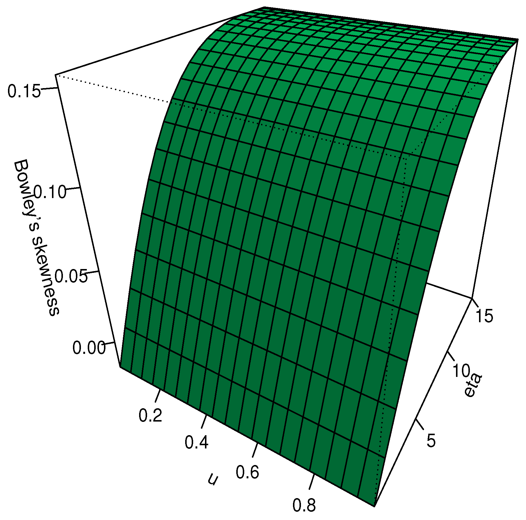
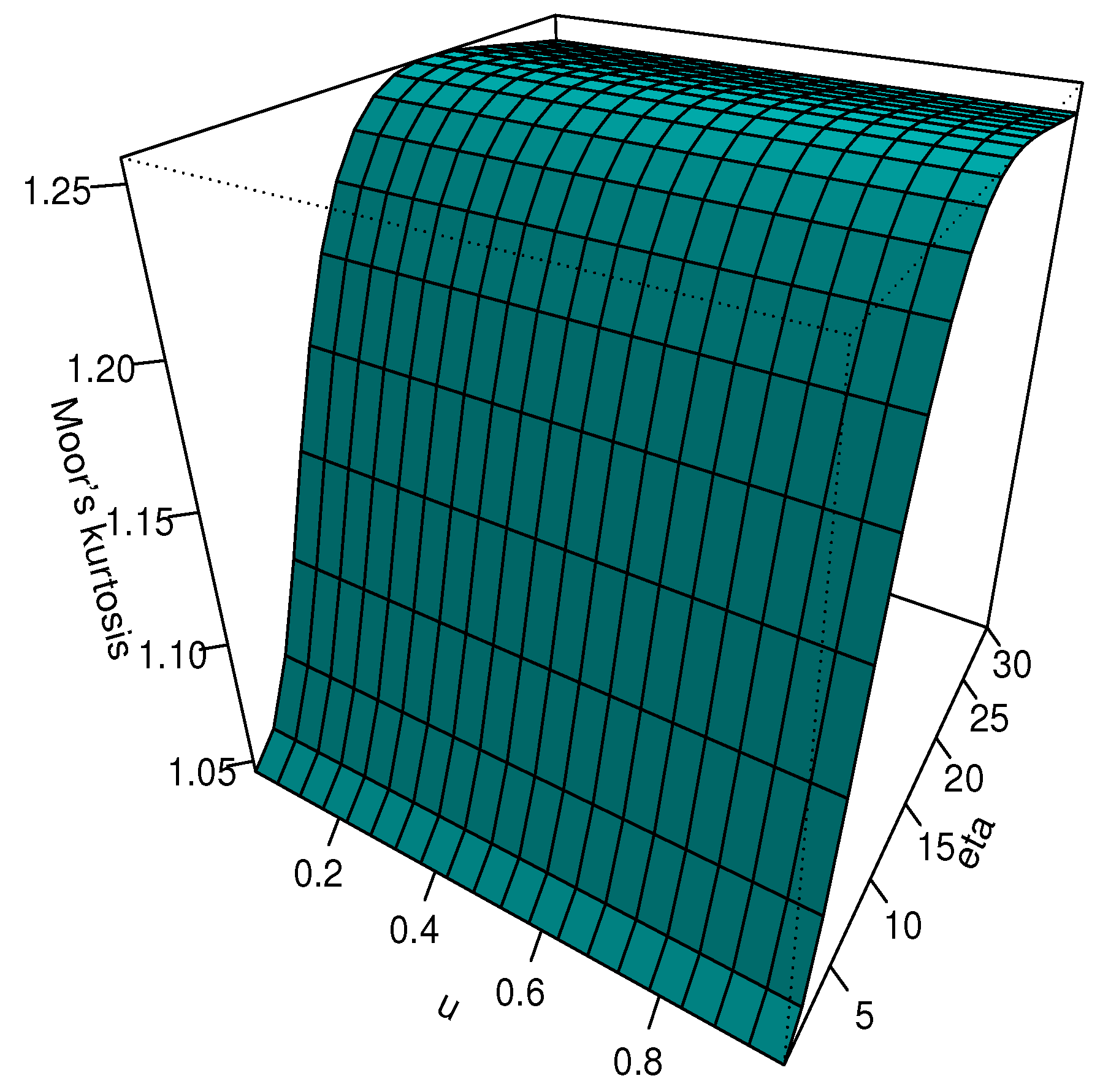
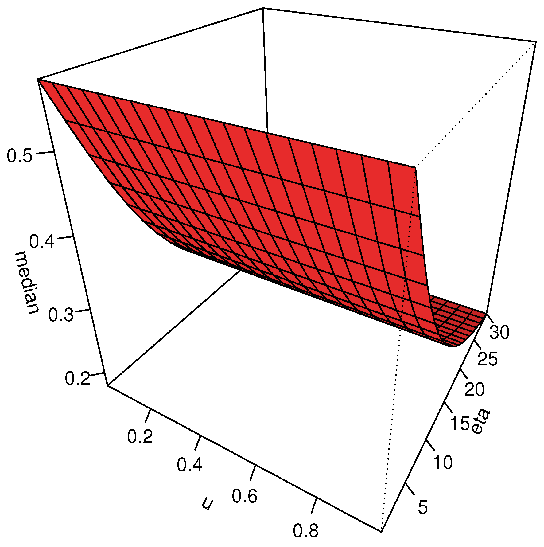
3.2. Quantile Function
3.3. Moments
3.4. Incomplete Moments
3.5. Probability Weighted Moments
4. Measures of Uncertainty
4.1. Different Measures of Entropy
- More variability is produced when the value of increases, and for a fixed value of , the values of , , and decrease, resulting in more variability, whereas the values of , and increase, resulting in more information.
- As the value of increases and for a fixed value of , the values of , , , and decrease, resulting in more variability, but the values of decrease and then increase, while the values of increase and then decrease.

| R** | ** | A** | T** | ** | ** | ** | ||
|---|---|---|---|---|---|---|---|---|
| 2 | −0.026 | −0.031 | −0.025 | −0.026 | −0.177 | 0.223 | −0.053 | |
| 5 | −0.035 | −0.042 | −0.035 | −0.035 | −0.329 | 0.432 | −0.088 | |
| 7 | −0.055 | −0.066 | −0.054 | −0.055 | −0.426 | 0.573 | −0.144 | |
| 10 | −0.102 | −0.120 | −0.097 | −0.100 | −0.544 | 0.754 | −0.261 | |
| 0.5 | 13 | −0.163 | −0.189 | −0.150 | −0.156 | −0.627 | 0.888 | −0.398 |
| 15 | −0.208 | −0.239 | −0.188 | −0.198 | −0.666 | 0.953 | −0.493 | |
| 20 | −0.329 | −0.366 | −0.280 | −0.303 | −0.722 | 1.049 | −0.721 | |
| 25 | −0.447 | −0.484 | −0.361 | −0.401 | −0.742 | 1.084 | −0.925 | |
| 27 | −0.492 | −0.527 | −0.389 | −0.436 | −0.744 | 1.089 | −1.000 | |
| 30 | −0.557 | −0.587 | −0.427 | −0.486 | −0.745 | 1.09 | −1.104 | |
| 2 | −0.036 | −0.048 | −0.036 | −0.036 | −0.167 | 0.228 | −0.046 | |
| 5 | −0.052 | −0.070 | −0.052 | −0.052 | −0.312 | 0.433 | −0.073 | |
| 7 | −0.084 | −0.112 | −0.083 | −0.083 | −0.398 | 0.557 | −0.118 | |
| 10 | −0.153 | −0.203 | −0.150 | −0.151 | −0.493 | 0.697 | −0.215 | |
| 0.8 | 13 | −0.239 | −0.313 | −0.232 | −0.233 | −0.551 | 0.784 | −0.328 |
| 15 | −0.300 | −0.391 | −0.289 | −0.291 | −0.574 | 0.819 | −0.406 | |
| 20 | −0.451 | −0.580 | −0.427 | −0.431 | −0.599 | 0.856 | −0.592 | |
| 25 | −0.589 | −0.747 | −0.547 | −0.555 | −0.600 | 0.858 | −0.756 | |
| 27 | −0.638 | −0.806 | −0.590 | −0.599 | −0.598 | 0.855 | −0.814 | |
| 30 | −0.708 | −0.888 | −0.649 | −0.660 | −0.594 | 0.848 | −0.895 | |
| 2 | −0.046 | −0.071 | −0.046 | −0.046 | −0.156 | 0.238 | −0.036 | |
| 5 | −0.072 | −0.113 | −0.073 | −0.073 | −0.292 | 0.438 | −0.052 | |
| 7 | −0.117 | −0.183 | −0.118 | −0.118 | −0.365 | 0.543 | −0.083 | |
| 10 | −0.210 | −0.331 | −0.214 | −0.215 | −0.436 | 0.645 | −0.151 | |
| 1.2 | 13 | −0.317 | −0.506 | −0.326 | −0.328 | −0.472 | 0.696 | −0.233 |
| 15 | −0.390 | −0.627 | −0.403 | −0.406 | −0.484 | 0.713 | −0.291 | |
| 20 | −0.560 | −0.915 | −0.587 | −0.592 | −0.490 | 0.722 | −0.431 | |
| 25 | −0.704 | −1.167 | −0.747 | −0.756 | −0.485 | 0.715 | −0.555 | |
| 27 | −0.754 | −1.258 | −0.804 | −0.814 | −0.482 | 0.711 | −0.599 | |
| 30 | −0.823 | −1.383 | −0.883 | −0.895 | −0.478 | 0.705 | −0.660 | |
| 2 | −0.052 | −0.090 | −0.052 | −0.053 | −0.150 | 0.247 | −0.026 | |
| 5 | −0.086 | −0.150 | −0.087 | −0.088 | −0.278 | 0.444 | −0.035 | |
| 7 | −0.139 | −0.246 | −0.142 | −0.144 | −0.342 | 0.537 | −0.055 | |
| 10 | −0.246 | −0.446 | −0.256 | −0.261 | −0.400 | 0.619 | −0.100 | |
| 1.5 | 13 | −0.363 | −0.680 | −0.386 | −0.398 | −0.426 | 0.655 | −0.156 |
| 15 | −0.441 | −0.842 | −0.475 | −0.493 | −0.433 | 0.665 | −0.198 | |
| 20 | −0.616 | −1.231 | −0.683 | −0.721 | −0.434 | 0.667 | −0.303 | |
| 25 | −0.760 | −1.579 | −0.865 | −0.925 | −0.429 | 0.659 | −0.401 | |
| 27 | −0.811 | −1.706 | −0.931 | −1.000 | −0.426 | 0.655 | −0.436 | |
| 30 | −0.879 | −1.885 | −1.022 | −1.104 | −0.422 | 0.650 | −0.486 |
4.2. Measures of Extropy
- When the value of increases, the values of the extropy and residual extropy decrease, providing more uncertainty.
- When the value of t increases and for a fixed value of , the residual extropy decreases, leading to more variability.
| Extropy | Residual Extropy | ||||||
|---|---|---|---|---|---|---|---|
| 2 | −0.531 | −0.564 | −0.723 | −1.010 | −1.674 | −2.505 | −5.003 |
| 5 | −0.556 | −0.600 | −0.778 | −1.060 | −1.707 | −2.527 | −5.014 |
| 7 | −0.593 | −0.648 | −0.841 | −1.115 | −1.743 | −2.552 | −5.026 |
| 10 | −0.671 | −0.747 | −0.970 | −1.229 | −1.817 | −2.602 | −5.051 |
| 13 | −0.763 | −0.866 | −1.130 | −1.374 | −1.914 | −2.668 | −5.085 |
| 15 | −0.827 | −0.952 | −1.249 | −1.486 | −1.991 | −2.722 | −5.112 |
| 20 | −0.988 | −1.176 | −1.577 | −1.808 | −2.223 | −2.884 | −5.195 |
| 25 | −1.142 | −1.401 | −1.928 | −2.172 | −2.504 | −3.087 | −5.301 |
| 27 | −1.200 | −1.491 | −2.071 | −2.325 | −2.627 | −3.178 | −5.350 |
| 30 | −1.284 | −1.624 | −2.287 | −2.560 | −2.823 | −3.326 | −5.429 |
5. Classical Estimation
5.1. Maximum Likelihood Estimation
5.2. Maximum Product of Spacings Estimation
6. Bayesian Estimation
- 1.
- Start with initial values .
- 2.
- Let
- 3.
- Use the M-H algorithm to generate from with the normal distributions .
- 4.
- Generate a required from . The choices of are thought to be the asymptotic V-CM, say , where is the FIM.
- (i)
- Find the acceptance probabilities
- (ii)
- From the uniform distribution, generate the value .
- (iii)
- If , accept the proposal and set ; otherwise set .
- 5.
- Set
- 6.
- Repeat steps (3)–(5) N times, and obtain ,
- 7.
- To compute the credible CI (C-CI) of as , then the C-CI of is
7. Numerical Outcomes
- Sch.1: and .
- Sch.2: , and .
- Sch.3: , , and , where r is an even number.
- Sch.4: and .
- (a)
- For the non-BE
- The RMSE and AL decrease when r increases for the ML and MPS approaches.
- In almost all situations, using the MPS, the RMSE of is smaller than the MSE of using ML.
- In almost all situations, using the ML, the RB of is smaller than the RB of using MPS.
- In most situations, using the ML, Sch.4 gives the lowest value of the MSE for .
- In most situations, using the ML, Sch.3 gives the lowest value of the RB for .
- In most situations, using the MPS, Sch.4 gives the smallest values of the RMSE and RB for .
- The CP is greater than or equal 91.30% at .
- In almost all situations, using the ML, Sch.4 gives the smallest AL for .
- In almost all situations, using the MPS, Sch.4 gives the smallest AL for .
- (b)
- For the BE
- The RMSE decreases when r increases for the MCMC method using the SE and LIN loss functions.
- The AL decreases when r increases for the MCMC method using the SE and LIN loss functions.
- In almost all situations, the RMSE and RB of using the IP is less than the RMSE of using the non-IP under the MCMC method using the SE and LIN loss functions.
- The RMSE of at is less than the RMSE of at in most of situations for the IP and non-IP.
- The RB of at is less than the RB of , and at , in almost all situations, for the non-IP.
- In almost all situations, the RB of is less than the RB of at and for the IP.
- In almost all situations, using the MCMC under the non-IP, Sch.4 gives the smallest values of the RMSE for .
- In almost all situations, using the MCMC under the non-IP, Sch.2 gives the smallest values of the RB for .
- In the majority of situations, the RB of at is less than the RMSE of and at for the IP and non-IP.
- In almost all situations, using the MCMC under the IP, Sch.4 gives the smallest values of the RMSEs for .
- In almost all situations, using the MCMC under the IP, Sch.3 gives the smallest values of the RB for .
- The CP is more than or equal 95.0% at .
- In almost all situations, using the MCMC under the non-IP, Sch.2 gives the lowest AL for .
- In almost all situations, using the MCMC under the IP, Sch.4 gives the lowest AL for .
- In almost all situations, using the MCMC, the AL under the IP is less than the AL under the non-IP for .
- In almost all situations, using the MCMC, the RMSE under the IP is less than the RMSE using the ML and MPS.
- In almost all situations, using the MCMC, the RB under the IP is less than the RB using the ML and MPS.
- In almost all situations, using the MCMC, the AL under the IP is less than the AL under the ML and MPS for .
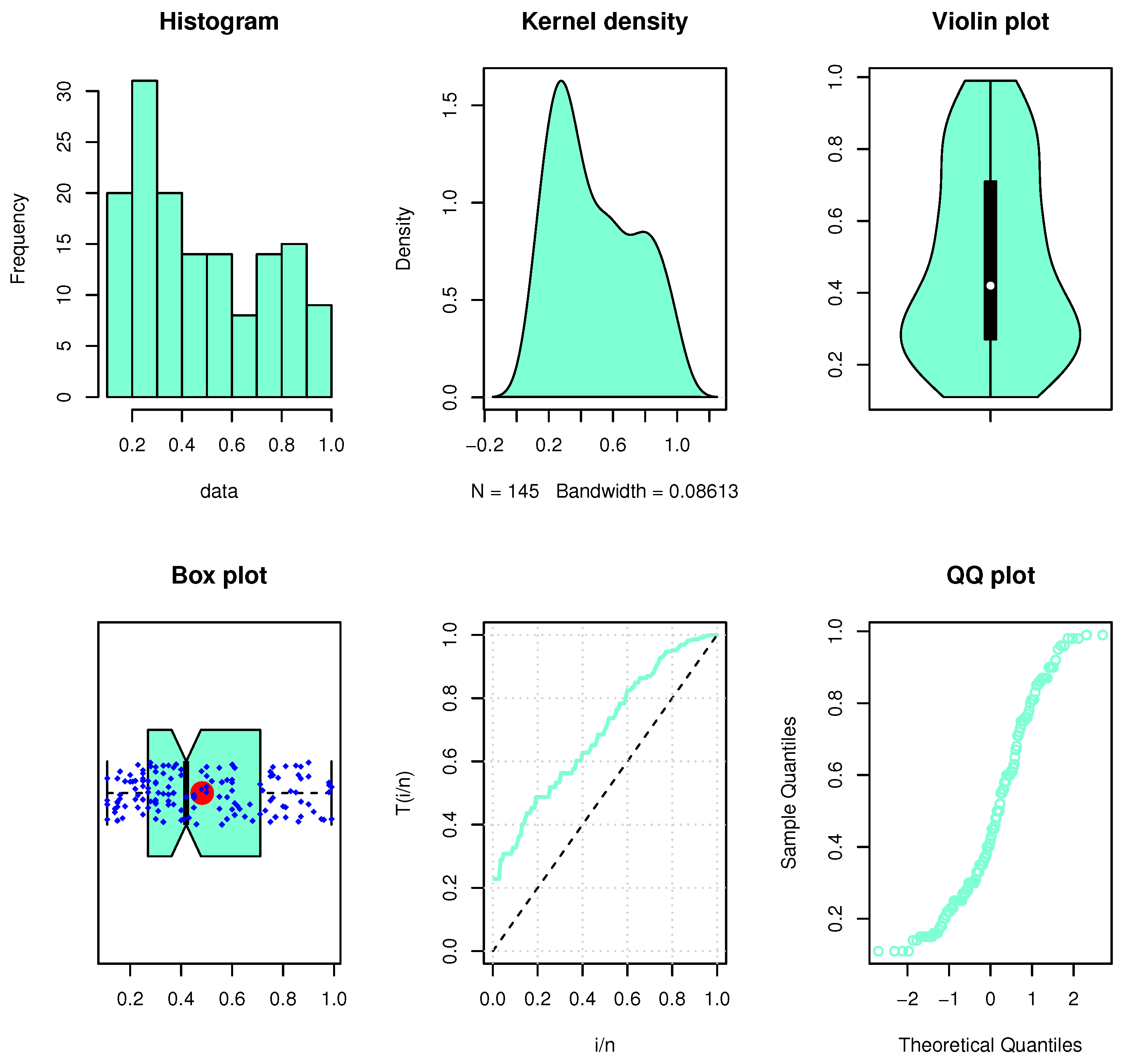
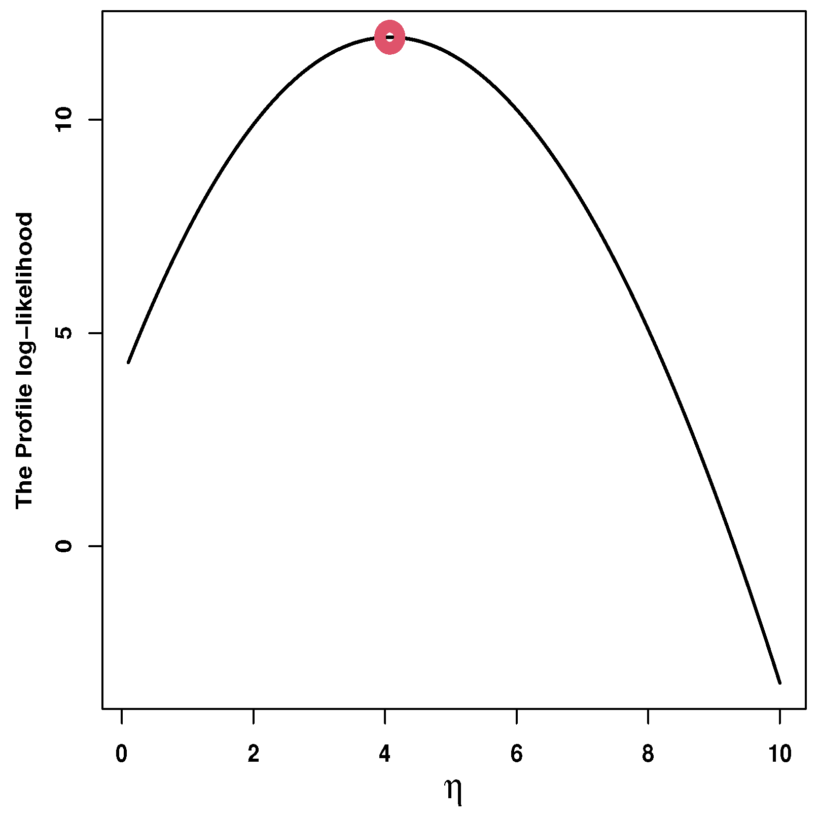
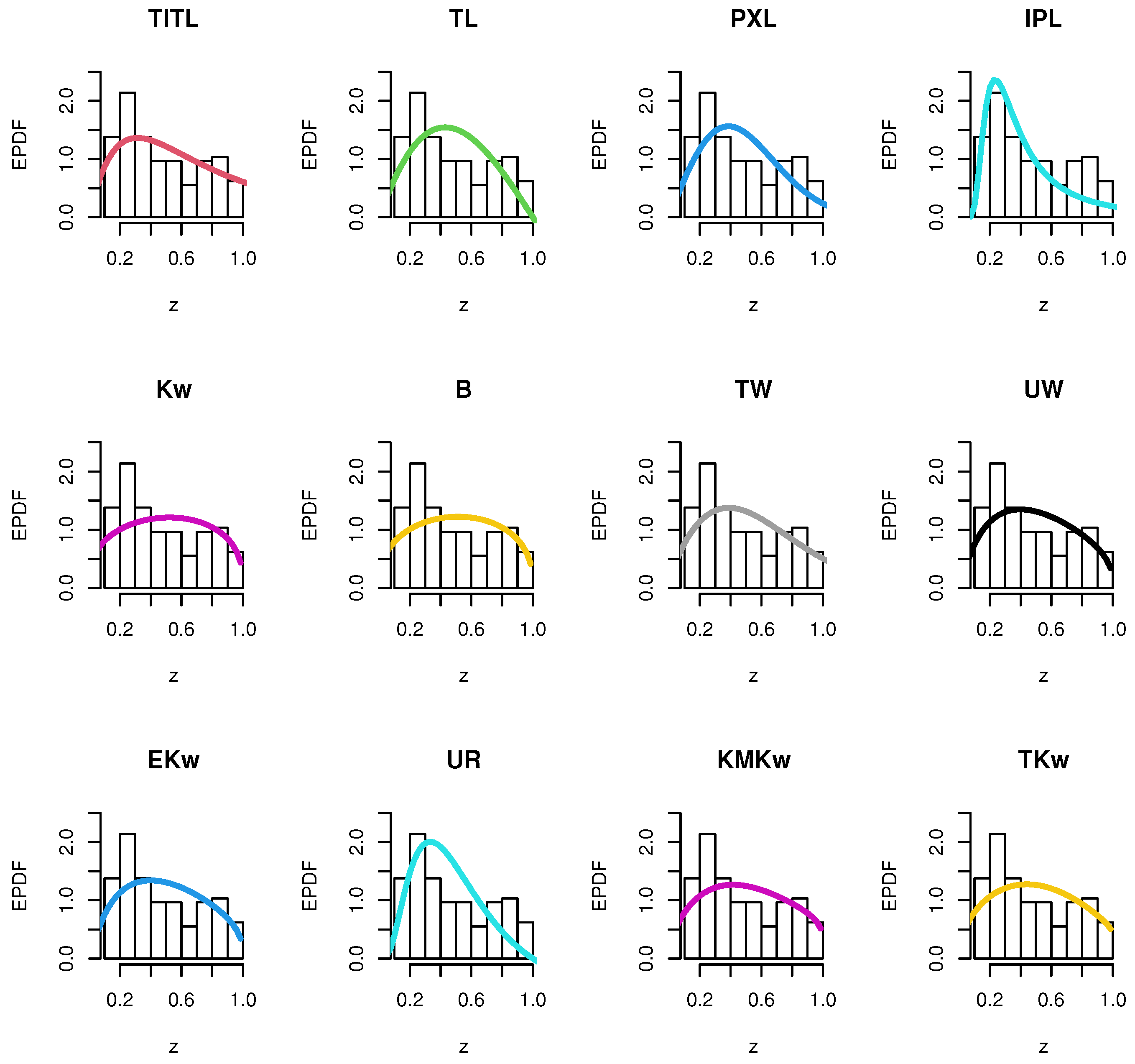
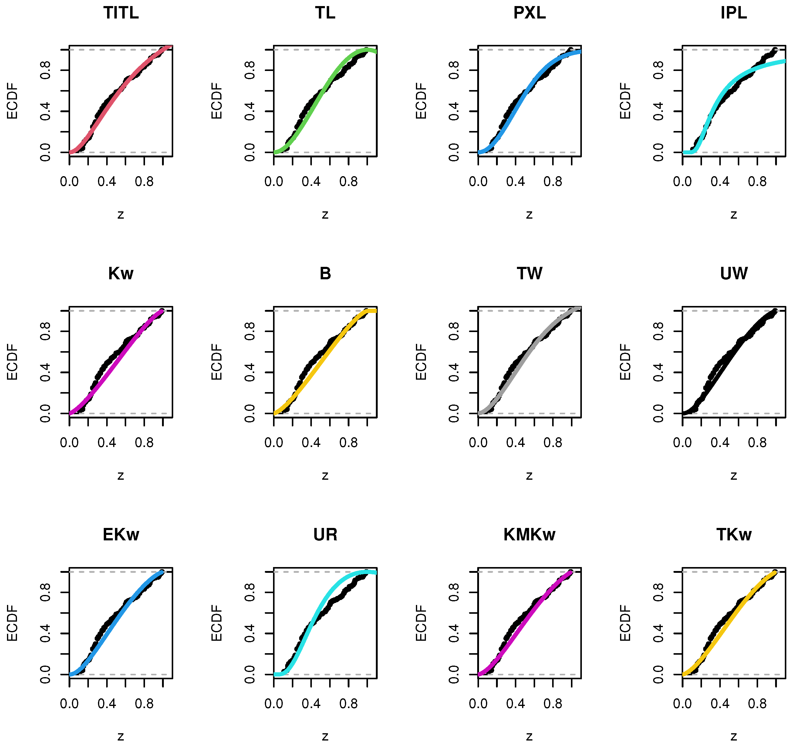
8. Applications
8.1. The First Dataset
8.2. The Second Dataset
9. Conclusions
Author Contributions
Funding
Data Availability Statement
Acknowledgments
Conflicts of Interest
References
- Topp, C.W.; Leone, F.C. A family of J-shaped frequency functions. J. Am. Stat. Assoc. 1955, 50, 209–219. [Google Scholar] [CrossRef]
- Al-Shomrani, A.; Arif, O.; Shawky, A.; Hanif, S.; Shahbaz, M.Q. Topp-Leone family of distributions: Some properties and application. Pak. J. Stat. Oper. Res. 2016, 12, 443–451. [Google Scholar] [CrossRef] [Green Version]
- Rezaei, S.; Sadr, B.B.; Alizadeh, M.; Nadarajah, S. Topp-Leone generated family of distributions: Properties and applications. Commun. Stat. Theory Methods 2016, 46, 2893–2909. [Google Scholar] [CrossRef]
- Sangsanit, Y.; Bodhisuwan, W. The Topp-Leone generator of distributions: Properties and inferences. Songklanakarin Sci. Technol. 2016, 38, 537–548. [Google Scholar]
- Yousof, H.M.; Alizadeh, M.; Jahanshahi, S.M.A.; Ramires, T.G.; Ghosh, I.; Hamedani, G.G. The Transmuted Topp-Leone G family of distributions: Theory, characterizations and applications. J. Data Sci. 2017, 15, 723–740. [Google Scholar] [CrossRef]
- Reyad, H.; Korkmaz, M.C.; Afify, A.Z.; Hamedani, G.G.; Othman, S. The Fréchet Topp-Leone-G family of distributions: Properties, characterizations and applications. Ann. Data Sci. 2019, 8, 345–366. [Google Scholar] [CrossRef]
- Reyad, H.M.; Alizadeh, M.; Jamal, F.; Othman, S.; Hamedani, G.G. The exponentiated generalized Topp Leone-G family of distributions: Properties and applications. Pak. J. Stats. Oper. Res. 2019, 15, 1–24. [Google Scholar] [CrossRef] [Green Version]
- Mahdavi, A. Generalized Topp-Leone family of distributions. Biostat. Epidemiol. 2017, 3, 65–75. [Google Scholar]
- Elgarhy, M.; Nasir, M.A.; Jamal, F.; Ozel, G. The type II Topp-Leone generated family of distributions: Properties and applications. J. Stat. Manag. Syst. 2018, 21, 1529–1551. [Google Scholar] [CrossRef]
- Bantan, R.A.; Jamal, F.; Chesneau, C.; Elgarhy, M. A new power Topp-Leone generated family of distributions with applications. Entropy 2019, 21, 1177. [Google Scholar] [CrossRef] [Green Version]
- Elgarhy, M.; Hassan, A.S.; Nagy, H. Parameter estimation methods and applications of the power Topp-Leone distribution. Gazi Univ. J. Sci. 2022, 35, 731–746. [Google Scholar] [CrossRef]
- Alizadeh, M.; Lak, F.; Rasekhi, M.; Ramires, T.G.; Yousof, H.M.; Altun, E. The odd log-logistic Topp-Leone G family of distributions: Heteroscedastic regression models and applications. Comput. Stat. 2018, 33, 1217–1244. [Google Scholar] [CrossRef]
- Chipepa, F.; Oluyede, B.; Peter, O.P. The Burr III-Topp-Leone-G family of distributions with applications. Heliyon 2021, 7, e06534. [Google Scholar] [CrossRef]
- Hassan, A.S.; Elgarhy, M.; Ragab, R. Statistical properties and estimation of inverted Topp-Leone distribution. J. Stat. Appl. Probab. 2020, 9, 319–331. [Google Scholar]
- Metwally, A.S.M.; Hassan, A.S.; Almetwally, E.M.; Kibria, B.M.G.; Almongy, H.M. Reliability analysis of the new exponential inverted Topp-Leone distribution with applications. Entropy 2021, 23, 1662. [Google Scholar] [CrossRef]
- Almetwally, E.M.; Alharbi, R.; Alnagar, D.; Hafez, E.H. A new inverted Topp-Leone distribution: Applications to the COVID-19 mortality rate in two different countries. Axioms 2021, 10, 25. [Google Scholar] [CrossRef]
- Mohamed, R.A.H.; Elgarhy, M.; Alabdulhadi, M.H.; Almetwally, E.M.; Radwan, T. Statistical inference of truncated Cauchy power-inverted Topp-Leone distribution under hybrid censored scheme with applications. Axioms 2023, 12, 148. [Google Scholar] [CrossRef]
- Mahdavi, A.; Silva, O.G. A method to expand family of continuous distributions based on truncated distributions. J. Stat. Res. Iran 2017, 13, 231–247. [Google Scholar] [CrossRef] [Green Version]
- Abid, S.H.; Abdulrazak, R.K. [0, 1] truncated Fréchet-G generator of distributions. Appl. Math. 2017, 7, 51–66. [Google Scholar]
- Bantan, R.A.R.; Jamal, F.; Chesneau, C.; Elgarhy, M. Truncated inverted Kumaraswamy generated family of distributions with applications. Entropy 2019, 21, 1089. [Google Scholar] [CrossRef] [Green Version]
- ZeinEldin, R.A.; Chesneau, C.; Jamal, F.; Elgarhy, M.; Almarashi, A.M.; Al-Marzouki, S. Generalized truncated Fréchet generated family distributions and their applications. Comput. Model. Eng. Sci. 2021, 126, 791–819. [Google Scholar]
- Almarashi, A.M.; Jamal, F.; Chesneau, C.; Elgarhy, M. A new truncated Muth generated family of distributions with applications. Complexity 2021, 2021, 1211526. [Google Scholar] [CrossRef]
- Balakrishnan, N.; Aggrawala, R. Progressive Censoring, Theory, Methods and Applications; Birkhauser: Boston, MA, USA, 2000. [Google Scholar]
- Abdel-Hamid, A.H. Properties, estimations and predictions for a Poisson-half-logistic distribution based on progressively type-II censored samples. Appl. Math. Model. 2016, 40, 7164–7181. [Google Scholar] [CrossRef]
- Kundu, D.; Joarder, A. Analysis of type-II progressively hybrid censored data. Comput. Stat. Data Anal. 2006, 50, 2509–2528. [Google Scholar] [CrossRef]
- Mohammed, H.S.; Nassar, M.; Alotaibi, R.; Elshahhat, A. Analysis of adaptive progressive Type-II hybrid censored Dagum data with applications. Symmetry 2022, 14, 2146. [Google Scholar] [CrossRef]
- Maiti, K.; Kayal, S. Estimation of parameters and reliability characteristics for a generalized Rayleigh distribution under progressive Type-II censored sample. Commun. Stat-Simul. Comput. 2021, 50, 3669–3698. [Google Scholar] [CrossRef]
- Lee, K.; Cho, Y. Bayesian and maximum likelihood estimations of the inverted exponentiated half logistic distribution under progressive Type II censoring. J. Appl. Stat. 2017, 44, 811–832. [Google Scholar] [CrossRef]
- Buzaridah, M.M.; Ramadan, D.A.; El-Desouky, B.S. Estimation of some lifetime parameters of flexible reduced logarithmic-inverse Lomax distribution under progressive Type-II censored data. J. Math. 2022, 2022, 1690458. [Google Scholar] [CrossRef]
- Alotaibi, R.; Almetwally, E.M.; Kumar, D.; Rezk, H. Optimal test plan of step-stress model of alpha power Weibull lifetimes under progressively Type-II censored samples. Symmetry 2022, 14, 1801. [Google Scholar] [CrossRef]
- Alotaibi, R.; Baharith, L.A.; Almetwally, E.M.; Khalifa, M.; Ghosh, I.; Rezk, H. Statistical inference on a Finite mixture of exponentiated Kumaraswamy-G distributions with progressive Type II censoring Using bladder cancer data. Mathematics 2022, 10, 2800. [Google Scholar] [CrossRef]
- Wang, L.; Wu, K.; Zuo, X. Inference and prediction of progressive Type-II censored data from unit-generalized Rayleigh distribution. Hacet. J. Math. Stat. 2022, 51, 1752–1767. [Google Scholar] [CrossRef]
- Tse, S.K.; Yang, C.; Yuen, H.K. Statistical analysis of Weibull distributed lifetime data under type II progressive censoring with binomial removals. J. Appl. Stat. 2020, 27, 1033–1043. [Google Scholar] [CrossRef]
- Salem, S.; Abo-Kasem, O.E.; Hussien, A. On joint Type-II generalized progressive hybrid censoring scheme. Comput. J. Math. Stat. Sci. 2023, 2, 123–158. [Google Scholar] [CrossRef]
- Kleiber, C.; Kotz, S. Statistical Size Distributions in Economics and Actuarial Sciences; Wiley: New York, NY, USA, 2023. [Google Scholar]
- Greenwood, J.A.L.; Landwehr, J.M.; Wallis, J.R.; Matals, N.C. Probability weighted moments: Definition and relation to parameters of several distributions expressable in inverse form. Water Resour. Res. 1979, 15, 1049–1054. [Google Scholar] [CrossRef] [Green Version]
- Rényi, A. On measures of entropy and information. In Proceedings of the 4th Berkeley Symposium on Mathematical Statistics and Probability, Berkeley, CA, USA, 20 June–30 July 1960; Volume 1, pp. 47–561. [Google Scholar]
- Tsallis, C. Possible generalization of Boltzmann-Gibbs statistics. J. Stat. Phys. 1988, 52, 479–487. [Google Scholar] [CrossRef]
- Arimoto, S. Information-theoretical considerations on estimation problems. Inf. Control 1971, 19, 181–194. [Google Scholar] [CrossRef] [Green Version]
- Havrda, J.; Charvat, F. Quantification method of classification processes, concept of structural a-entropy. Kybernetika 1967, 3, 30–35. [Google Scholar]
- Awad, A.M.; Alawneh, A.J. Application of entropy to a life-time model. Ima J. Math. Control Inf. 1987, 4, 143–148. [Google Scholar] [CrossRef]
- Mathai, A.M.; Haubold, H.J. On generalized distributions and pathways. Phys. Lett. 2008, 372, 2109–2113. [Google Scholar] [CrossRef] [Green Version]
- Lad, F.; Sanfilippo, G.; Agro, G. Extropy: Complementary dual of entropy. Stat. Sci. 2015, 30, 40–58. [Google Scholar] [CrossRef]
- Shannon, C.E. A mathematical theory of communication. Bell Syst. Tech. J. 1948, 27, 379–423. [Google Scholar] [CrossRef] [Green Version]
- Qiu, G.; Jia, K. The residual extropy of order statistics. Stat. Probab. Lett. 2018, 133, 15–22. [Google Scholar] [CrossRef]
- Cohen, A.C. Progressively censored samples in life testing. Technometrics 1963, 5, 327–329. [Google Scholar] [CrossRef]
- Cheng, R.C.H.; Amin, N.A.K. Estimating parameters in continuous univariate distributions with a shifted origin. J. R. Stat. Soc. Ser. B. 1983, 45, 394–403. [Google Scholar] [CrossRef]
- Coolen, F.P.A.; Newby, M.J. A Note on the Use of the Product of Spacings in Bayesian Inference; Department of Mathematics and Computing Science University of Technology: Eindhoven, The Netherlands, 1990. [Google Scholar]
- Anatolyev, S.; Kosenok, G. An alternative to maximum likelihood based on spacings. Econ. Theory 2005, 21, 472–476. [Google Scholar] [CrossRef] [Green Version]
- Ng, H.K.T.; Luo, L.; Hu, Y.; Duan, F. Parameter estimation of three-parameter Weibull distribution based on progressively type-II censored samples. Stat Comput. Simul. 2012, 82, 1661–1678. [Google Scholar] [CrossRef]
- Dey, S.; Dey, T.; Luckett, D.J. Statistical inference for the generalized inverted exponential distribution based on upper record values. Math. Comput. Simul. 2016, 120, 64–78. [Google Scholar] [CrossRef]
- Meriem, B.; Gemeay, A.M.; Almetwally, E.M.; Halim, Z.; Alshawarbeh, E.; Abdulrahman, A.T.; Hussam, E. The power xlindley distribution: Statistical inference, fuzzy reliability, and covid-19 application. J. Funct. Spaces 2022, 2022, 9094078. [Google Scholar] [CrossRef]
- Barco, K.V.P.; Mazucheli, J.; Janeiro, V. The inverse power Lindley distribution. Commun. Stat.-Simul. Comput. 2017, 46, 6308–6323. [Google Scholar] [CrossRef]
- Kumaraswamy, P. A Generalized Probability Density Function for Double-Bounded Random Processes. J. Hydrol. 1980, 46, 79–88. [Google Scholar] [CrossRef]
- Gupta, A.K.; Nadarajah, S. Handbook of Beta Distribution and Its Applications; CRC Press: Boca Raton, FL, USA, 2004. [Google Scholar]
- Najarzadegan, H.; Alamatsaz, M.H.; Hayati, S. Truncated Weibull-G more flexible and more reliable than beta-G distribution. Int. J. Stat. Probab. 2017, 6, 1–17. [Google Scholar] [CrossRef] [Green Version]
- Mazucheli, J.; Menezes, A.F.B.; Ghitany, M.E. The unit-Weibull distribution and associated inference. J. Appl. Probab. Stat. 2018, 13, 1–22. [Google Scholar]
- Lemonte, A.J.; Barreto-Souza, W.; Cordeiro, G.M. The exponentiated Kumaraswamy distribution and its log-transform. Braz. J. Probab. Stat. 2013, 27, 3153. [Google Scholar] [CrossRef]
- Bantan, R.A.; Chesneau, C.; Jamal, F.; Elgarhy, M.; Tahir, M.H.; Ali, A.; Anam, S. Some new facts about the unit-Rayleigh distribution with applications. Mathematics 2020, 8, 1954. [Google Scholar] [CrossRef]
- Alotaibi, N.; Elbatal, I.; Shrahili, M.; Al-Moisheer, A.S.; Elgarhy, M.; Almetwally, E.M. Statistical inference for the Kavya-Manoharan Kumaraswamy model under ranked set sampling with applications. Symmetry 2023, 15, 587. [Google Scholar] [CrossRef]
- Khan, M.S.; King, R.; Hudson, I.L. Transmuted Kumaraswamy distribution. Stat. Transit. New Ser. 2016, 2, 183–210. [Google Scholar] [CrossRef] [Green Version]
- Klein, J.P.; Moeschberger, M.L. Survival Analysis: Techniques for Censored and Truncated Data; Springer: Berlin/Heidelberg, Germany, 2006. [Google Scholar]


| 2 | 0.311 | 0.517 | 0.738 | 0.036 | 1.06 |
| 5 | 0.256 | 0.434 | 0.653 | 0.103 | 1.117 |
| 7 | 0.227 | 0.387 | 0.595 | 0.13 | 1.162 |
| 10 | 0.195 | 0.331 | 0.516 | 0.151 | 1.215 |
| 13 | 0.171 | 0.289 | 0.45 | 0.156 | 1.244 |
| 15 | 0.158 | 0.267 | 0.415 | 0.155 | 1.253 |
| 20 | 0.135 | 0.226 | 0.348 | 0.149 | 1.256 |
| 25 | 0.12 | 0.198 | 0.302 | 0.142 | 1.252 |
| 27 | 0.115 | 0.189 | 0.288 | 0.14 | 1.25 |
| 30 | 0.108 | 0.178 | 0.27 | 0.136 | 1.248 |
| Mode | |||||||||
|---|---|---|---|---|---|---|---|---|---|
| 2 | 0.524 | 0.341 | 0.25 | 0.196 | 0.067 | 0.036 | 1.935 | 0.494 | 0.408 |
| 5 | 0.462 | 0.277 | 0.191 | 0.144 | 0.063 | 0.299 | 2.097 | 0.545 | 0.289 |
| 7 | 0.424 | 0.239 | 0.158 | 0.115 | 0.059 | 0.461 | 2.308 | 0.573 | 0.250 |
| 10 | 0.373 | 0.19 | 0.117 | 0.081 | 0.051 | 0.679 | 2.742 | 0.606 | 0.213 |
| 13 | 0.331 | 0.152 | 0.086 | 0.056 | 0.043 | 0.86 | 3.256 | 0.628 | 0.189 |
| 15 | 0.307 | 0.132 | 0.071 | 0.044 | 0.038 | 0.956 | 3.606 | 0.636 | 0.177 |
| 20 | 0.26 | 0.095 | 0.044 | 0.025 | 0.028 | 1.113 | 4.36 | 0.643 | 0.154 |
| 25 | 0.227 | 0.072 | 0.029 | 0.014 | 0.021 | 1.172 | 4.807 | 0.638 | 0.139 |
| 27 | 0.216 | 0.065 | 0.025 | 0.012 | 0.019 | 1.177 | 4.898 | 0.635 | 0.134 |
| 30 | 0.202 | 0.057 | 0.021 | 0.009 | 0.016 | 1.172 | 4.961 | 0.63 | 0.127 |
| Sch. | Measures | Non-Bayesian | Bayesian | |||||||
|---|---|---|---|---|---|---|---|---|---|---|
| ML | MPS | Non-IP | IP | |||||||
| SE | LIN | SE | LIN | |||||||
| Sch.1 | Avg | 1.7694 | 1.8546 | 1.1726 | 1.0625 | 1.2905 | 1.6736 | 1.6148 | 1.8143 | |
| RMSE | 1.6327 | 1.6299 | 1.7446 | 1.6739 | 1.8287 | 1.3017 | 1.2445 | 1.3564 | ||
| RB | 0.1796 | 0.2364 | 0.2183 | 0.2900 | 0.1400 | 0.1157 | 0.0800 | 0.2100 | ||
| Sch.2 | Avg | 1.6812 | 1.6661 | 0.9769 | 0.8560 | 1.1097 | 1.5611 | 1.4730 | 1.6610 | |
| RMSE | 1.2507 | 1.1929 | 1.4258 | 1.3867 | 1.4812 | 0.9954 | 0.9397 | 1.0680 | ||
| RB | 0.1208 | 0.1107 | 0.3487 | 0.4300 | 0.2600 | 0.0407 | 0.0200 | 0.1100 | ||
| Sch.3 | Avg | 1.7016 | 1.8839 | 1.0272 | 0.9106 | 1.1593 | 1.6430 | 1.5266 | 1.7421 | |
| RMSE | 1.4085 | 1.3915 | 1.5492 | 1.5102 | 1.6084 | 1.1102 | 1.0653 | 1.1701 | ||
| RB | 0.1344 | 0.2559 | 0.3152 | 0.3900 | 0.2300 | 0.0953 | 0.0200 | 0.1600 | ||
| Sch.4 | Avg | 1.6995 | 1.7175 | 1.0276 | 0.9111 | 1.1610 | 1.4931 | 1.4370 | 1.6328 | |
| RMSE | 1.2424 | 1.1621 | 1.4444 | 1.4211 | 1.4853 | 1.0441 | 1.0001 | 1.0809 | ||
| RB | 0.1330 | 0.1450 | 0.3149 | 0.3900 | 0.2300 | 0.0046 | 0.0400 | 0.0900 | ||
| Sch.1 | Avg | 1.5696 | 1.6641 | 0.9890 | 0.8983 | 1.0885 | 1.5629 | 1.4895 | 1.6885 | |
| RMSE | 1.3337 | 1.2882 | 1.5135 | 1.4817 | 1.5554 | 1.0253 | 0.9627 | 1.0877 | ||
| RB | 0.0464 | 0.1094 | 0.3407 | 0.4000 | 0.2700 | 0.0419 | 0.0100 | 0.1300 | ||
| Sch.2 | Avg | 1.6398 | 1.7147 | 1.0468 | 0.9462 | 1.1554 | 1.6197 | 1.5064 | 1.7123 | |
| RMSE | 1.1640 | 1.1310 | 1.3791 | 1.3523 | 1.4140 | 1.0063 | 0.9712 | 1.0716 | ||
| RB | 0.0932 | 0.1431 | 0.3021 | 0.3700 | 0.2300 | 0.0798 | 0.0000 | 0.1400 | ||
| Sch.3 | Avg | 1.5682 | 1.6259 | 0.9768 | 0.8728 | 1.0902 | 1.5582 | 1.5166 | 1.6445 | |
| RMSE | 1.2199 | 1.2100 | 1.3919 | 1.3636 | 1.4350 | 1.0381 | 0.9891 | 1.0736 | ||
| RB | 0.0455 | 0.0839 | 0.3488 | 0.4200 | 0.2700 | 0.0388 | 0.0100 | 0.1000 | ||
| Sch.4 | Avg | 1.5909 | 1.6244 | 1.0180 | 0.9260 | 1.1191 | 1.5809 | 1.5248 | 1.7182 | |
| RMSE | 1.2355 | 1.1635 | 1.4526 | 1.4209 | 1.4955 | 0.9692 | 0.9179 | 0.9983 | ||
| RB | 0.0606 | 0.0829 | 0.3213 | 0.3800 | 0.2500 | 0.0540 | 0.0200 | 0.1500 | ||
| Sch.1 | Avg | 1.5914 | 1.6617 | 1.0325 | 0.9343 | 1.1392 | 1.4841 | 1.4393 | 1.6312 | |
| RMSE | 1.1465 | 1.0981 | 1.3969 | 1.3737 | 1.4320 | 0.9343 | 0.8840 | 0.9596 | ||
| RB | 0.0610 | 0.1078 | 0.3116 | 0.3800 | 0.2400 | 0.0106 | 0.0400 | 0.0900 | ||
| Sch.2 | Avg | 1.6240 | 1.6316 | 1.0430 | 0.9455 | 1.1482 | 1.6870 | 1.6031 | 1.7511 | |
| RMSE | 1.0374 | 0.9869 | 1.2554 | 1.2428 | 1.2776 | 0.9575 | 0.9037 | 1.0206 | ||
| RB | 0.0827 | 0.0878 | 0.3046 | 0.3700 | 0.2300 | 0.1247 | 0.0700 | 0.1700 | ||
| Sch.3 | Avg | 1.4956 | 1.6016 | 0.9448 | 0.8546 | 1.0418 | 1.4674 | 1.3837 | 1.5495 | |
| RMSE | 1.0593 | 0.9811 | 1.2496 | 1.2410 | 1.2673 | 0.8229 | 0.8043 | 0.8590 | ||
| RB | 0.0030 | 0.0677 | 0.3701 | 0.4300 | 0.3100 | 0.0217 | 0.0800 | 0.0300 | ||
| Sch.4 | Avg | 1.5119 | 1.5242 | 0.9381 | 0.8393 | 1.0469 | 1.4186 | 1.3454 | 1.4571 | |
| RMSE | 0.9886 | 0.9308 | 1.2163 | 1.2159 | 1.2264 | 0.8380 | 0.8210 | 0.8848 | ||
| RB | 0.0079 | 0.0161 | 0.3746 | 0.4400 | 0.3000 | 0.0543 | 0.1000 | 0.0300 | ||
| Sch.1 | Avg | 1.5384 | 1.6169 | 0.8937 | 0.8034 | 0.9924 | 1.4882 | 1.3955 | 1.5833 | |
| RMSE | 1.0634 | 0.9900 | 1.2371 | 1.2285 | 1.2574 | 0.8772 | 0.8564 | 0.9154 | ||
| RB | 0.0256 | 0.0780 | 0.4042 | 0.4600 | 0.3400 | 0.0079 | 0.0700 | 0.0600 | ||
| Sch.2 | Avg | 1.5997 | 1.6211 | 0.9914 | 0.8996 | 1.0920 | 1.4423 | 1.3615 | 1.5286 | |
| RMSE | 0.9215 | 0.9025 | 1.1910 | 1.1917 | 1.1980 | 0.8258 | 0.8060 | 0.8574 | ||
| RB | 0.0665 | 0.0807 | 0.3391 | 0.4000 | 0.2700 | 0.0385 | 0.0900 | 0.0200 | ||
| Sch.3 | Avg | 1.5219 | 1.5614 | 0.8847 | 0.7977 | 0.9802 | 1.4203 | 1.3354 | 1.4787 | |
| RMSE | 0.9114 | 0.8739 | 1.1818 | 1.1836 | 1.1906 | 0.7534 | 0.7431 | 0.7858 | ||
| RB | 0.0146 | 0.0409 | 0.4102 | 0.4700 | 0.3500 | 0.0531 | 0.1100 | 0.0100 | ||
| Sch.4 | Avg | 1.4641 | 1.4990 | 0.8610 | 0.7822 | 0.9460 | 1.4294 | 1.3860 | 1.4859 | |
| RMSE | 0.9213 | 0.8396 | 1.1646 | 1.1714 | 1.1643 | 0.7557 | 0.7247 | 0.7723 | ||
| RB | 0.0239 | 0.0007 | 0.4260 | 0.4800 | 0.3700 | 0.0471 | 0.0800 | 0.0100 | ||
| Sch. | Measures | Non-Bayesian | Bayesian | |||||||
|---|---|---|---|---|---|---|---|---|---|---|
| ML | MPS | Non-IP | IP | |||||||
| SE | LIN | SE | LIN | |||||||
| Sch.1 | Avg | 3.1857 | 3.3117 | 2.5174 | 2.3583 | 2.6805 | 3.0145 | 2.8488 | 3.1843 | |
| RMSE | 1.6952 | 1.7022 | 2.2439 | 2.2420 | 2.2573 | 1.1379 | 1.1050 | 1.2020 | ||
| RB | 0.0619 | 0.1039 | 0.1609 | 0.2100 | 0.1100 | 0.0048 | 0.0500 | 0.0600 | ||
| Sch.2 | Avg | 3.0733 | 3.0361 | 2.4320 | 2.2468 | 2.6287 | 3.0112 | 2.8591 | 3.1665 | |
| RMSE | 1.5074 | 1.4077 | 2.0734 | 2.0853 | 2.0827 | 1.1064 | 1.0845 | 1.1608 | ||
| RB | 0.0244 | 0.0120 | 0.1893 | 0.2500 | 0.1200 | 0.0037 | 0.0500 | 0.0600 | ||
| Sch.3 | Avg | 3.1584 | 3.2552 | 2.5072 | 2.3500 | 2.6671 | 3.0299 | 2.8700 | 3.1955 | |
| RMSE | 1.5976 | 1.5722 | 2.1247 | 2.1190 | 2.1452 | 1.0900 | 1.0606 | 1.1519 | ||
| RB | 0.0528 | 0.0851 | 0.1643 | 0.2200 | 0.1100 | 0.0100 | 0.0400 | 0.0700 | ||
| Sch.4 | Avg | 2.9309 | 2.8805 | 2.2926 | 2.1375 | 2.4544 | 2.9092 | 2.7593 | 3.0618 | |
| RMSE | 1.5531 | 1.4300 | 2.1900 | 2.1889 | 2.1992 | 1.0662 | 1.0634 | 1.0945 | ||
| RB | 0.0230 | 0.0398 | 0.2358 | 0.2900 | 0.1800 | 0.0303 | 0.0800 | 0.0200 | ||
| Sch.1 | Avg | 3.0399 | 3.1030 | 2.2936 | 2.1307 | 2.4655 | 3.0083 | 2.8487 | 3.1692 | |
| RMSE | 1.4542 | 1.4628 | 2.0123 | 2.0296 | 2.0089 | 1.0493 | 1.0244 | 1.1052 | ||
| RB | 0.0133 | 0.0343 | 0.2355 | 0.2900 | 0.1800 | 0.0028 | 0.0500 | 0.0600 | ||
| Sch.2 | Avg | 3.0791 | 3.0884 | 2.5252 | 2.3634 | 2.6957 | 3.0375 | 2.8905 | 3.1880 | |
| RMSE | 1.5008 | 1.3427 | 2.0200 | 2.0248 | 2.0284 | 1.2183 | 1.1874 | 1.2697 | ||
| RB | 0.0264 | 0.0295 | 0.1583 | 0.2100 | 0.1000 | 0.0125 | 0.0400 | 0.0600 | ||
| Sch.3 | Avg | 3.1232 | 3.1737 | 2.4937 | 2.3233 | 2.6754 | 2.9741 | 2.8318 | 3.1208 | |
| RMSE | 1.3495 | 1.3469 | 1.9196 | 1.9285 | 1.9281 | 1.0471 | 1.0272 | 1.0917 | ||
| RB | 0.0411 | 0.0579 | 0.1688 | 0.2300 | 0.1100 | 0.0086 | 0.0600 | 0.0400 | ||
| Sch.4 | Avg | 2.9834 | 2.9780 | 2.3157 | 2.1516 | 2.4875 | 2.9074 | 2.7616 | 3.0555 | |
| RMSE | 1.2857 | 1.2024 | 1.8625 | 1.8930 | 1.8452 | 0.9258 | 0.9217 | 0.9612 | ||
| RB | 0.0055 | 0.0073 | 0.2281 | 0.2800 | 0.1700 | 0.0309 | 0.0800 | 0.0200 | ||
| Sch.1 | Avg | 2.9100 | 2.9386 | 2.1268 | 1.9754 | 2.2821 | 2.8911 | 2.7592 | 3.0249 | |
| RMSE | 1.2443 | 1.2555 | 1.9211 | 1.9512 | 1.8988 | 0.9155 | 0.9199 | 0.9310 | ||
| RB | 0.0300 | 0.0205 | 0.2911 | 0.3400 | 0.2400 | 0.0363 | 0.0800 | 0.0100 | ||
| Sch.2 | Avg | 2.8227 | 2.8668 | 2.3326 | 2.1872 | 2.4829 | 2.9339 | 2.8118 | 3.0577 | |
| RMSE | 1.2312 | 1.0460 | 1.6599 | 1.6879 | 1.6458 | 0.8421 | 0.8377 | 0.8654 | ||
| RB | 0.0591 | 0.0444 | 0.2225 | 0.2700 | 0.1700 | 0.0220 | 0.0600 | 0.0200 | ||
| Sch.3 | Avg | 3.0518 | 3.0979 | 2.4813 | 2.3155 | 2.6512 | 2.9538 | 2.8356 | 3.0757 | |
| RMSE | 1.1745 | 1.1385 | 1.6552 | 1.6873 | 1.6377 | 0.8944 | 0.8953 | 0.9121 | ||
| RB | 0.0173 | 0.0326 | 0.1729 | 0.2300 | 0.1200 | 0.0154 | 0.0500 | 0.0300 | ||
| Sch.4 | Avg | 3.0054 | 2.9491 | 2.4945 | 2.3379 | 2.6565 | 2.9293 | 2.8131 | 3.0480 | |
| RMSE | 1.0441 | 0.9971 | 1.5006 | 1.5525 | 1.4655 | 0.8225 | 0.8234 | 0.8447 | ||
| RB | 0.0018 | 0.0170 | 0.1685 | 0.2200 | 0.1100 | 0.0236 | 0.0600 | 0.0200 | ||
| Sch.1 | Avg | 3.0491 | 3.0710 | 2.5690 | 2.4049 | 2.7384 | 2.9325 | 2.8090 | 3.0578 | |
| RMSE | 1.0803 | 1.0890 | 1.5435 | 1.5884 | 1.5166 | 0.9277 | 0.9234 | 0.9503 | ||
| RB | 0.0164 | 0.0237 | 0.1437 | 0.2000 | 0.0900 | 0.0225 | 0.0600 | 0.0200 | ||
| Sch.2 | Avg | 2.9620 | 2.9742 | 2.5609 | 2.4179 | 2.7083 | 2.9301 | 2.8176 | 3.0444 | |
| RMSE | 0.9560 | 0.8874 | 1.3854 | 1.4229 | 1.3661 | 0.7808 | 0.7798 | 0.8019 | ||
| RB | 0.0127 | 0.0086 | 0.1464 | 0.1900 | 0.1000 | 0.0233 | 0.0600 | 0.0100 | ||
| Sch.3 | Avg | 2.9919 | 3.0252 | 2.5167 | 2.3757 | 2.6583 | 2.9099 | 2.7998 | 3.0213 | |
| RMSE | 1.0398 | 1.0098 | 1.4560 | 1.4891 | 1.4409 | 0.8384 | 0.8366 | 0.8584 | ||
| RB | 0.0027 | 0.0084 | 0.1611 | 0.2100 | 0.1100 | 0.0300 | 0.0700 | 0.0100 | ||
| Sch.4 | Avg | 3.0546 | 3.0421 | 2.6801 | 2.5430 | 2.8199 | 2.9415 | 2.8323 | 3.0527 | |
| RMSE | 0.9185 | 0.8724 | 1.2904 | 1.3226 | 1.2744 | 0.7526 | 0.7579 | 0.7667 | ||
| RB | 0.0182 | 0.0140 | 0.1066 | 0.1500 | 0.0600 | 0.0195 | 0.0600 | 0.0200 | ||
| Sch. | Asy-CI | C-CI | |||||||
|---|---|---|---|---|---|---|---|---|---|
| ML | MPS | Non-IP | IP | ||||||
| AL | CP | AL | CP | AL | CP | AL | CP | ||
| Sch.1 | 3.9669 | 91.30 | 5.0978 | 96.00 | 4.8511 | 95.30 | 4.1933 | 95.40 | |
| Sch.2 | 3.9723 | 97.30 | 4.4908 | 98.30 | 3.8292 | 95.20 | 3.6945 | 95.20 | |
| Sch.3 | 4.0224 | 95.00 | 4.6183 | 98.20 | 4.2337 | 95.40 | 3.7491 | 96.50 | |
| Sch.4 | 4.0418 | 97.30 | 4.1896 | 98.20 | 3.9481 | 95.00 | 3.3572 | 95.00 | |
| Sch.1 | 3.4406 | 92.30 | 4.4736 | 98.30 | 4.0581 | 95.30 | 3.4969 | 95.90 | |
| Sch.2 | 4.0052 | 98.30 | 4.18 | 98.90 | 3.7449 | 95.00 | 3.6709 | 95.80 | |
| Sch.3 | 3.5526 | 95.00 | 4.0874 | 97.60 | 3.6224 | 95.30 | 3.5855 | 95.20 | |
| Sch.4 | 3.4021 | 94.00 | 3.9504 | 96.90 | 3.9395 | 95.20 | 3.3492 | 95.20 | |
| Sch.1 | 3.2903 | 93.33 | 3.9173 | 97.33 | 3.7283 | 95.27 | 3.3874 | 95.32 | |
| Sch.2 | 3.1681 | 95.33 | 3.4049 | 97.97 | 3.4248 | 95.24 | 3.3308 | 96.38 | |
| Sch.3 | 3.0185 | 93.67 | 3.4255 | 96.93 | 3.2714 | 95.21 | 3.0017 | 95.07 | |
| Sch.4 | 3.0123 | 95.67 | 3.1343 | 96.22 | 3.1363 | 95.17 | 2.9732 | 95.50 | |
| Sch.1 | 2.8741 | 92.67 | 3.3921 | 97.67 | 3.1682 | 95.33 | 3.0918 | 95.69 | |
| Sch.2 | 3.1814 | 96.00 | 3.2003 | 96.25 | 3.0873 | 95.22 | 2.9764 | 95.18 | |
| Sch.3 | 2.8884 | 95.67 | 3.1556 | 97.00 | 2.9926 | 95.32 | 2.7684 | 95.06 | |
| Sch.4 | 2.6618 | 92.67 | 2.9786 | 97.65 | 2.9186 | 95.29 | 2.8176 | 95.58 | |
| Sch. | Asy-CI | C-CI | |||||||
|---|---|---|---|---|---|---|---|---|---|
| ML | MPS | Non-IP | IP | ||||||
| AL | CP | AL | CP | AL | CP | AL | CP | ||
| Sch.1 | 6.0590 | 97.00 | 6.1989 | 96.94 | 6.5888 | 95.24 | 3.9302 | 95.92 | |
| Sch.2 | 5.1527 | 96.33 | 5.3652 | 97.67 | 5.8769 | 95.33 | 4.0306 | 96.33 | |
| Sch.3 | 5.4113 | 96.67 | 5.5617 | 96.63 | 6.3835 | 95.29 | 3.8114 | 96.30 | |
| Sch.4 | 4.6693 | 94.67 | 4.9554 | 96.67 | 6.1642 | 95.33 | 3.8919 | 96.30 | |
| Sch.1 | 5.2310 | 98.33 | 5.3245 | 98.32 | 5.5444 | 95.30 | 3.8680 | 96.30 | |
| Sch.2 | 4.7743 | 95.32 | 4.9354 | 95.65 | 5.8743 | 95.30 | 4.3126 | 95.32 | |
| Sch.3 | 4.9676 | 97.00 | 5.0530 | 97.00 | 5.7158 | 95.33 | 3.7499 | 96.33 | |
| Sch.4 | 4.6157 | 97.67 | 4.7183 | 97.65 | 5.1431 | 95.30 | 3.3610 | 96.64 | |
| Sch.1 | 4.5177 | 96.70 | 4.5753 | 96.70 | 5.2294 | 95.30 | 3.1906 | 97.00 | |
| Sch.2 | 3.7061 | 95.70 | 3.9551 | 97.70 | 4.6005 | 95.30 | 3.0899 | 96.00 | |
| Sch.3 | 4.0586 | 95.30 | 4.1348 | 96.00 | 5.1036 | 95.30 | 3.2155 | 96.00 | |
| Sch.4 | 3.6459 | 95.60 | 3.7428 | 96.70 | 4.6793 | 95.30 | 2.8018 | 95.70 | |
| Sch.1 | 3.9742 | 96.70 | 3.9908 | 96.70 | 5.0981 | 95.70 | 3.1734 | 95.70 | |
| Sch.2 | 3.6055 | 97.70 | 3.6837 | 98.30 | 4.4782 | 95.30 | 2.9590 | 96.30 | |
| Sch.3 | 3.6442 | 98.00 | 3.6969 | 98.00 | 4.6904 | 95.30 | 2.9808 | 96.00 | |
| Sch.4 | 3.4424 | 96.70 | 3.4879 | 97.70 | 4.5827 | 95.30 | 2.7998 | 98.30 | |
| Distributions | MLE | SEr | ||||
|---|---|---|---|---|---|---|
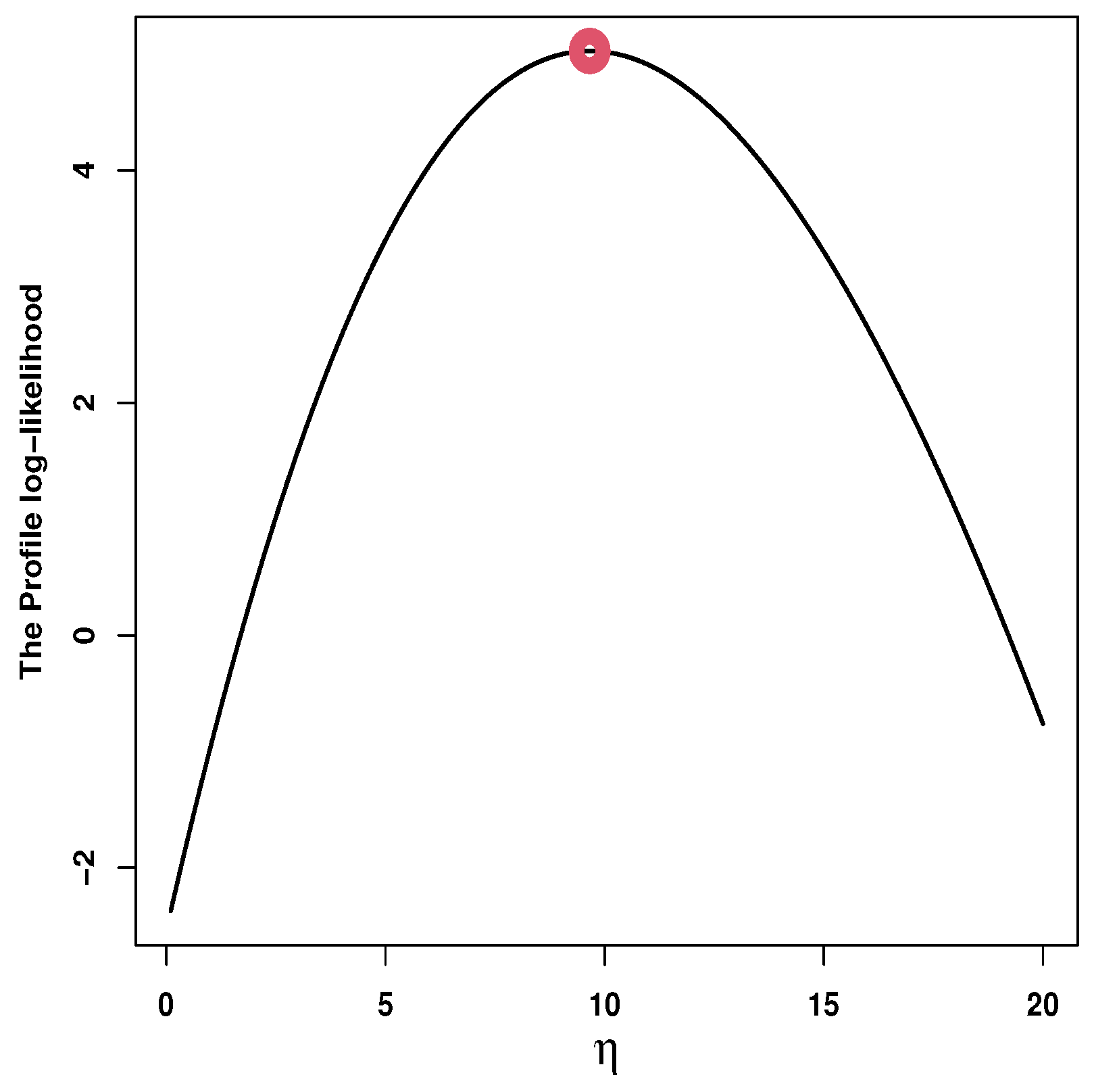
| TITL | 9.6584 | - | - | (2.7069) | - | - |
| TL | 1.3778 | - | - | (0.2604) | - | - |
| PXL | 1.637 | 4.2239 | - | (0.2409) | (0.9428) | - |
| IPL | 1.1641 | 0.3153 | - | (0.1421) | (0.0827) | - |
| Kw | 1.265 | 2.0797 | - | (0.2544) | (0.5714) | - |
| B | 1.3567 | 2.1058 | - | (0.3332) | (0.5496) | - |
| TW | 3.3328 | 1.5218 | - | (1.1901) | (0.2712) | - |
| UW | 0.6124 | 1.6991 | - | (0.1424) | (0.2669) | - |
| EKw | 0.0146 | 1.7156 | 868.6461 | (0.0135) | (0.2635) | (1354.074) |
| UR | 0.5222 | - | - | (0.0987) | - | - |
| KMKw | 1.4419 | 1.867 | - | (0.2706) | (0.5664) | - |
| TKw | 1.3879 | 1.7814 | 0.4852 | (0.2695) | (0.7043) | (0.4496) |
| Models | AIC | BIC | CAIC | HQIC | KS | PKS | ||
|---|---|---|---|---|---|---|---|---|
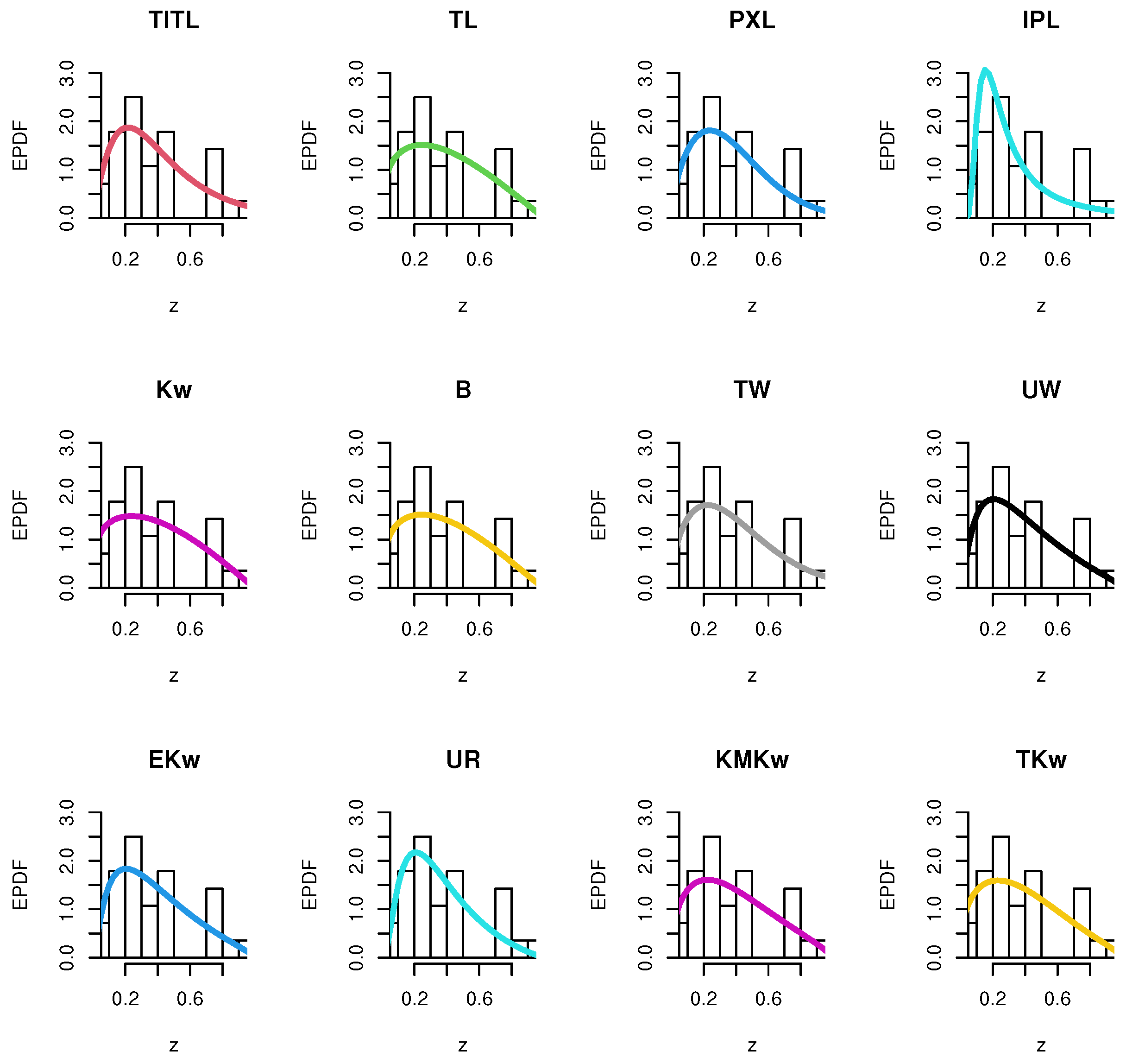
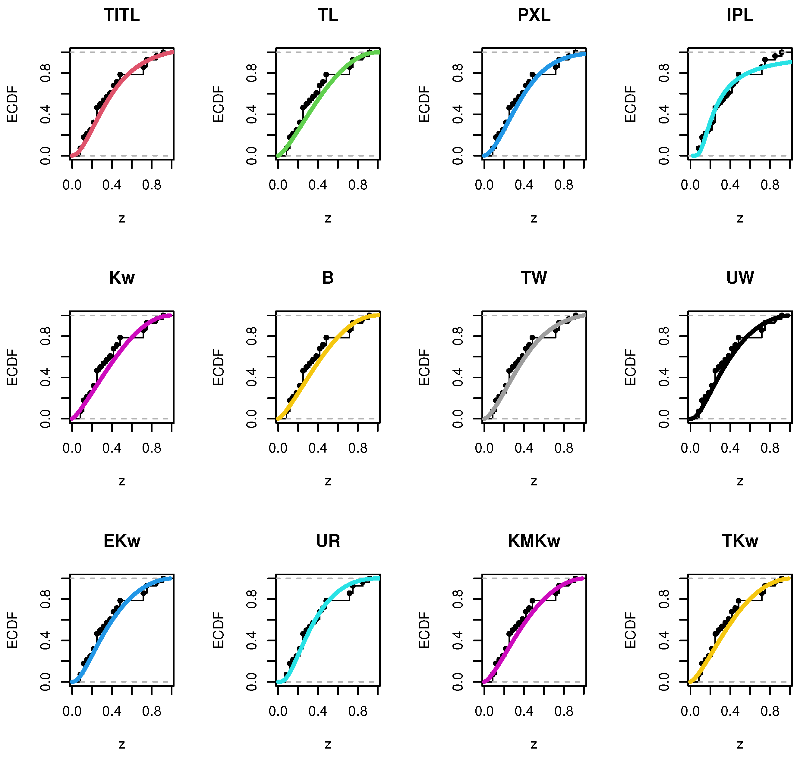
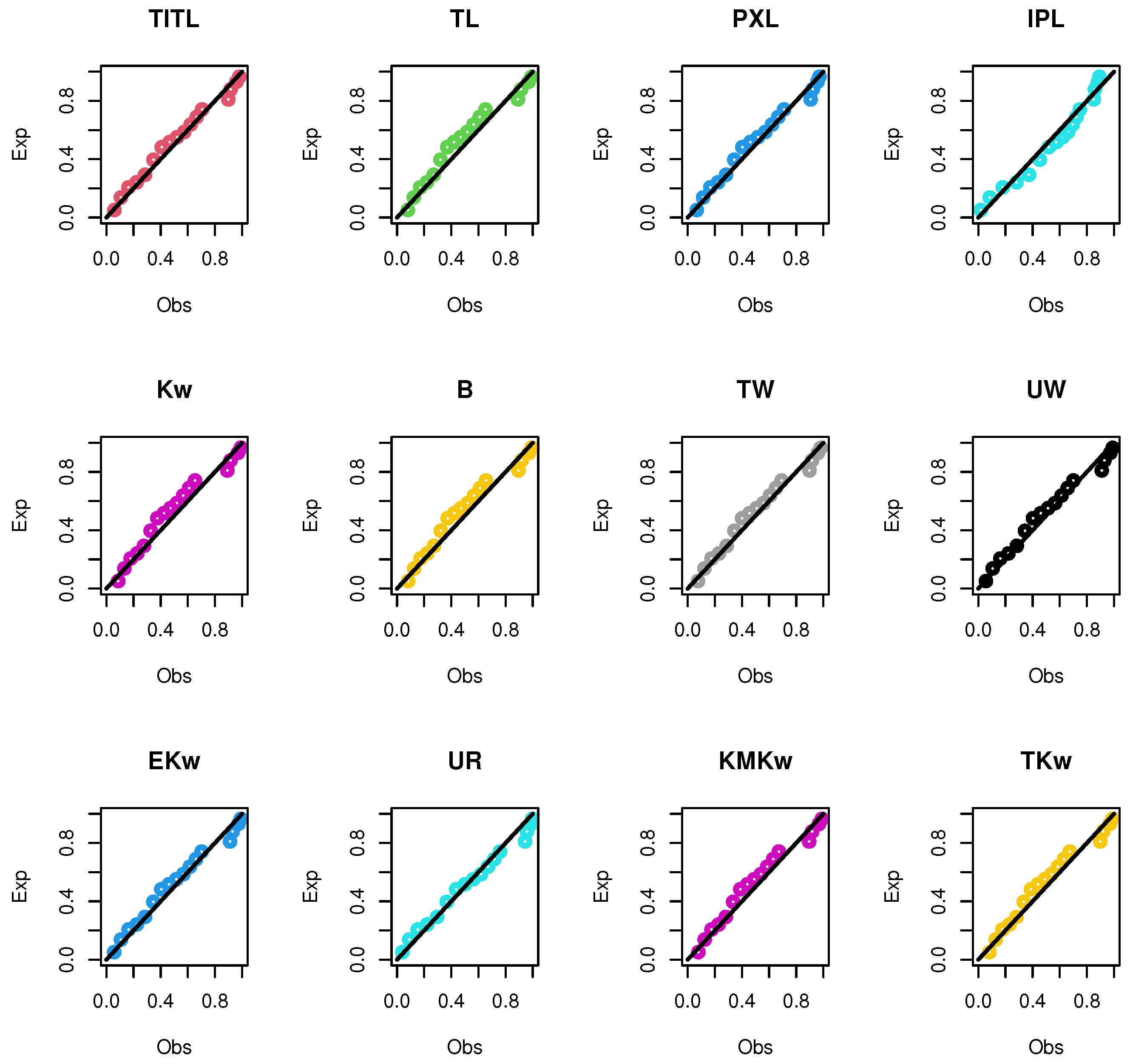
| TITL | −8.0555 | −6.7233 | −7.9017 | −7.6482 | 0.11687 | 0.83901 | 0.0533 | 0.386 |
| TL | −5.7049 | −4.3727 | −5.551 | −5.2976 | 0.14415 | 0.60568 | 0.1067 | 0.6679 |
| PXL | −3.5549 | −0.8905 | −3.0749 | −2.7404 | 0.12081 | 0.80843 | 0.0627 | 0.465 |
| IPL | 0.2734 | 2.9378 | 0.7534 | 1.0879 | 0.13099 | 0.72263 | 0.1012 | 0.7071 |
| Kw | −3.325 | −0.6606 | −2.845 | −2.5104 | 0.13772 | 0.66296 | 0.1136 | 0.7049 |
| B | −3.5552 | −0.8908 | −3.0752 | −2.7407 | 0.14118 | 0.63213 | 0.1101 | 0.6859 |
| TW | −4.8828 | −2.2184 | −4.4028 | −4.0683 | 0.1195 | 0.81882 | 0.0712 | 0.4882 |
| UW | −6.1223 | −3.4579 | −5.6423 | −5.3077 | 0.124 | 0.78239 | 0.066 | 0.4415 |
| EKw | −4.0392 | −0.0426 | −3.0392 | −2.8174 | 0.12535 | 0.77113 | 0.067 | 0.4475 |
| UR | −6.965 | −5.6328 | −6.8112 | −6.5578 | 0.15798 | 0.48692 | 0.0857 | 0.4132 |
| KMKw | −4.5907 | −1.9263 | −4.1107 | −3.7762 | 0.12921 | 0.73815 | 0.09 | 0.5785 |
| TKw | −2.2297 | 1.7669 | −1.2297 | −1.0079 | 0.12939 | 0.73658 | 0.0942 | 0.6043 |
| Sch. | Methods | Point Estimation | Interval Estimation | ||
|---|---|---|---|---|---|
| Estimate | SEr | LB | UB | ||
| Sch.1 | ML | 8.7305 | 2.8327 | 3.1784 | 14.2825 |
| MPS | 8.4375 | 2.6270 | 3.2887 | 13.5863 | |
| Bayesian at SE | 6.7562 | 1.3419 | 4.1858 | 9.9519 | |
| Bayesian at LIN | 6.3493 | ||||
| Bayesian at LIN | 7.2675 | ||||
| Sch.2 | ML | 8.7305 | 2.8327 | 3.1784 | 14.2825 |
| MPS | 8.4375 | 2.6270 | 3.2887 | 13.5863 | |
| Bayesian at SE | 6.7562 | 1.3419 | 4.1858 | 9.9519 | |
| Bayesian at LIN | 6.3493 | ||||
| Bayesian at LIN | 7.2675 | ||||
| Sch.3 | ML | 7.1133 | 2.6262 | 1.9661 | 12.2604 |
| MPS | 6.7383 | 2.4336 | 1.9685 | 11.5081 | |
| Bayesian at SE | 4.9507 | 1.3278 | 2.4091 | 8.0893 | |
| Bayesian at LIN | 4.5502 | ||||
| Bayesian at LIN | 5.4473 | ||||
| Sch.4 | ML | 8.7305 | 2.8327 | 3.1784 | 14.2825 |
| MPS | 8.4375 | 2.6270 | 3.2887 | 13.5863 | |
| Bayesian at SE | 6.7562 | 1.3419 | 4.1858 | 9.9519 | |
| Bayesian at LIN | 6.3493 | ||||
| Bayesian at LIN | 7.2675 | ||||
| Country | TE | Country | TE | Country | TE |
|---|---|---|---|---|---|
| Norway | 99 | Mauritius | 60 | Swaziland | 30 |
| Sweden | 99 | Mexico | 60 | Tanzania | 30 |
| European Union | 98 | Kazakhstan | 58 | Togo | 30 |
| Singapore | 98 | Panama | 58 | Zambia | 30 |
| United States | 98 | Uruguay | 58 | Cameroon | 28 |
| Austria | 96 | Cyprus | 56 | Mongolia | 28 |
| Finland | 96 | India | 56 | Turkey | 28 |
| New Zealand | 95 | Colombia | 55 | Bosnia and Herzegovina | 27 |
| France | 92 | Montserrat | 55 | Cape Verde | 27 |
| Hong Kong | 90 | Romania | 55 | Kyrgyzstan | 27 |
| Taiwan | 90 | Aruba | 52 | Papua New Guinea | 27 |
| United Arab Emirates | 90 | Azerbaijan | 50 | Angola | 25 |
| Belgium | 87 | Morocco | 50 | Bolivia | 25 |
| Isle of Man | 87 | San Marino | 50 | Gabon | 25 |
| Macau | 87 | Trinidad and Tobago | 50 | Madagascar | 25 |
| United Kingdom | 87 | Paraguay | 48 | Moldova | 25 |
| Qatar | 86 | Serbia | 48 | Nicaragua | 25 |
| South Korea | 86 | Greece | 46 | Solomon Islands | 25 |
| Cayman Islands | 85 | Georgia | 45 | St Vincent & Grenadines | 25 |
| Czech Republic | 85 | Guatemala | 45 | Tajikistan | 25 |
| Estonia | 83 | Macedonia | 45 | Iraq | 23 |
| Ireland | 81 | Vietnam | 45 | Nigeria | 23 |
| Israel | 81 | Oman | 43 | Tunisia | 23 |
| Kuwait | 81 | Brazil | 42 | Barbados | 22 |
| China | 80 | South Africa | 41 | Congo | 22 |
| Bermuda | 78 | Bangladesh | 40 | Maldives | 22 |
| Japan | 77 | Dominican Republic | 40 | Pakistan | 21 |
| Lithuania | 76 | Ivory Coast | 40 | Burkina Faso | 20 |
| Saudi Arabia | 76 | Namibia | 40 | Ecuador | 20 |
| Slovakia | 76 | Uzbekistan | 38 | Mozambique | 18 |
| Chile | 75 | Bahamas | 37 | Republic of the Congo | 18 |
| Iceland | 75 | Honduras | 37 | Belize | 17 |
| Malta | 75 | Senegal | 37 | El Salvador | 16 |
| Slovenia | 75 | Jordan | 36 | Ethiopia | 16 |
| Latvia | 73 | Albania | 35 | Ghana | 16 |
| Portugal | 72 | Fiji | 35 | Argentina | 15 |
| Poland | 71 | Montenegro | 35 | Cuba | 15 |
| Spain | 71 | Seychelles | 35 | Laos | 15 |
| Malaysia | 68 | Turkmenistan | 35 | Mali | 15 |
| Botswana | 67 | Bahrain | 33 | Suriname | 15 |
| Thailand | 65 | Benin | 33 | Ukraine | 15 |
| Andorra | 63 | Jamaica | 33 | Armenia | 14 |
| Italy | 62 | Rwanda | 33 | Russia | 14 |
| Bulgaria | 61 | Costa Rica | 31 | Belarus | 11 |
| Peru | 61 | Uganda | 31 | Lebanon | 11 |
| Philippines | 61 | Cambodia | 30 | Sri Lanka | 11 |
| Croatia | 60 | Egypt | 30 | Venezuela | 11 |
| Hungary | 60 | Kenya | 30 | ||
| Indonesia | 60 | Lesotho | 30 |
| Distributions | MLE | SEr | ||||
|---|---|---|---|---|---|---|
| TITL | 4.0725 | - | - | (1.0342) | - | - |
| TL | 2.0397 | - | - | (0.1694) | - | - |
| PXL | 1.989 | 3.4907 | - | (0.1317) | (0.3172) | - |
| IPL | 1.3356 | 0.3777 | - | (0.0714) | (0.0403) | - |
| Kw | 1.3552 | 1.3722 | - | (0.1319) | (0.1534) | - |
| B | 1.4096 | 1.3895 | - | (0.1555) | (0.153) | - |
| TW | 2.0867 | 1.7079 | - | (0.4652) | (0.1568) | - |
| UW | 1.0519 | 1.3462 | - | (0.0902) | (0.0939) | - |
| EKw | 0.0084 | 1.3441 | 647.545 | (0.0032) | (0.0925) | (401.9746) |
| UR | 0.8683 | - | - | (0.0721) | - | - |
| KMKw | 1.5544 | 1.1978 | - | (0.1402) | (0.1478) | - |
| TKw | 1.4985 | 1.1078 | 0.5516 | (0.1396) | (0.1999) | (0.2078) |
| Models | AIC | BIC | CAIC | HQIC | KS | PKS | ||
|---|---|---|---|---|---|---|---|---|
| TITL | −21.8691 | −18.8924 | −21.8411 | −20.6596 | 0.0706 | 0.46518 | 0.2192 | 1.3184 |
| TL | 6.6854 | 9.6622 | 6.7134 | 7.895 | 0.11114 | 0.05564 | 0.3701 | 2.2434 |
| PXL | 1.7966 | 7.7501 | 1.8812 | 4.2157 | 0.09056 | 0.1853 | 0.2868 | 1.8143 |
| IPL | 36.2007 | 42.1542 | 36.2852 | 38.6198 | 0.12858 | 0.01655 | 0.4778 | 3.3536 |
| Kw | −5.387 | 0.5664 | −5.3025 | −2.968 | 0.11684 | 0.03817 | 0.4012 | 2.4364 |
| B | −5.9722 | −0.0187 | −5.8877 | −3.5531 | 0.11783 | 0.03567 | 0.3947 | 2.3972 |
| TW | −15.6395 | −9.686 | −15.555 | −13.2204 | 0.09274 | 0.16499 | 0.2733 | 1.6344 |
| UW | −13.9249 | −7.9714 | −13.8404 | −11.5058 | 0.10304 | 0.09199 | 0.291 | 1.7599 |
| EKw | −11.7021 | −2.7719 | −11.5319 | −8.0735 | 0.10306 | 0.09188 | 0.2948 | 1.7832 |
| UR | 22.2578 | 25.2345 | 22.2857 | 23.4673 | 0.16523 | 0.00073 | 0.2738 | 1.7402 |
| KMKw | −12.3769 | −6.4234 | −12.2924 | −9.9578 | 0.10565 | 0.07854 | 0.3144 | 1.9033 |
| TKw | −8.9 | 0.0302 | −8.7298 | −5.2713 | 0.10629 | 0.07554 | 0.336 | 2.0198 |
| Sch. | Methods | Point Estimation | Interval Estimation | ||
|---|---|---|---|---|---|
| Estimate | SEr | LB | UB | ||
| Sch.1 | ML | 3.06563 | 1.5164 | 0.0936 | 6.0377 |
| MPS | 3.12188 | 1.5297 | 0.1237 | 6.1200 | |
| Bayesian at SE | 0.50815 | 0.7391 | 0.0000 | 2.2492 | |
| Bayesian at LIN | 0.39678 | ||||
| Bayesian at LIN | 0.67640 | ||||
| Sch.2 | ML | 3.81 × | 0.1077 | 0.0000 | 0.2111 |
| MPS | 1.34 × | 0.2080 | 0.0000 | 0.4076 | |
| Bayesian at SE | 0.00628 | 0.0291 | 0.0332 | ||
| Bayesian at LIN | 0.00608 | ||||
| Bayesian at LIN | 0.00650 | ||||
| Sch.3 | ML | 0.00031 | 0.4417 | 0.0000 | 0.8661 |
| MPS | 0.00031 | 0.9955 | 0.0000 | 1.9514 | |
| Bayesian at SE | 0.09273 | 0.2754 | 0.0000 | 0.8017 | |
| Bayesian at LIN | 0.07649 | ||||
| Bayesian at LIN | 0.11514 | ||||
| Sch.4 | ML | 3.81 × | 0.0239 | 0.0000 | 0.0467 |
| MPS | 1.34 × | 0.2063 | 0.0000 | 0.4043 | |
| Bayesian at SE | 0.00524 | 0.0184 | 0.0000 | 0.0298 | |
| Bayesian at LIN | 0.00516 | ||||
| Bayesian at LIN | 0.00533 | ||||
Disclaimer/Publisher’s Note: The statements, opinions and data contained in all publications are solely those of the individual author(s) and contributor(s) and not of MDPI and/or the editor(s). MDPI and/or the editor(s) disclaim responsibility for any injury to people or property resulting from any ideas, methods, instructions or products referred to in the content. |
© 2023 by the authors. Licensee MDPI, Basel, Switzerland. This article is an open access article distributed under the terms and conditions of the Creative Commons Attribution (CC BY) license (https://creativecommons.org/licenses/by/4.0/).
Share and Cite
Elgarhy, M.; Alsadat, N.; Hassan, A.S.; Chesneau, C.; Abdel-Hamid, A.H. A New Asymmetric Modified Topp–Leone Distribution: Classical and Bayesian Estimations under Progressive Type-II Censored Data with Applications. Symmetry 2023, 15, 1396. https://doi.org/10.3390/sym15071396
Elgarhy M, Alsadat N, Hassan AS, Chesneau C, Abdel-Hamid AH. A New Asymmetric Modified Topp–Leone Distribution: Classical and Bayesian Estimations under Progressive Type-II Censored Data with Applications. Symmetry. 2023; 15(7):1396. https://doi.org/10.3390/sym15071396
Chicago/Turabian StyleElgarhy, Mohammed, Najwan Alsadat, Amal S. Hassan, Christophe Chesneau, and Alaa H. Abdel-Hamid. 2023. "A New Asymmetric Modified Topp–Leone Distribution: Classical and Bayesian Estimations under Progressive Type-II Censored Data with Applications" Symmetry 15, no. 7: 1396. https://doi.org/10.3390/sym15071396