1. Introduction
The stress–strength, which was initially proposed by Birnbaum [
1] and developed by Birnbaum and McCarty [
2], plays an important role in reliability analysis. For two independent random variables,
X and
Y, the stress–strength parameter is defined as
. If stress
Y is greater than strength
X, it may result in component failure or system malfunction. The stress–strength parameter is originally used in the industrial field to calculate the reliability of the products [
3,
4]. It is also increasingly used to estimate the probability that one variable exceeds another [
5,
6], which is of great significance in practical application and has been widely used in various fields, such as electrical cable failure analysis, leukemia treatment, and jute fiber testing. See more details for [
5,
7,
8,
9,
10].
In the literature, there are many life distributions that can be used to estimate
R, such as Weibull [
5], Pareto [
6,
11], generalized Pareto [
12], exponential [
8,
13], generalized exponential [
14], Lomax [
15], unit-half-normal [
16], unit-Gompertz [
17], and generalized logistic (GL) [
18,
19,
20,
21] distributions. The logistic distribution is a symmetric heavy-tailed distribution. However, it is not suitable for handling asymmetric or thin-tailed data. Therefore, it is necessary to further extend the logistic distribution according to practical problems, which can handle the data including symmetric, heavy-tailed, asymmetric, and thin-tailed. The GL distribution, as defined by Balakrishnan and Leung [
22], is one of the generalized forms of the standard logistic distribution. By introducing a shape parameter to the distribution, the GL distribution expands the range of values for the skewness coefficient and tail index, which allows a wider range of data fitting capabilities. It has attracted extensive attention and is widely used in various fields, including demography, biology, finance, and neural network, as detailed in [
23]. Therefore, we select the GL distribution with the following probability density function (PDF)
and the corresponding cumulative distribution function (CDF) is
where
and
are the scale and shape parameters, respectively. The GL distribution exhibits a negative skew when
and a positive skew when
, and it becomes the standard logistic distribution (it is symmetric) when
. Meanwhile, the PDF of the GL distribution is unimodal and log-concave, making it suitable for modeling data with both left and right skewness [
18]. The expectation and variance of
X can be calculated from the moment-generating function of the GL distribution [
24]; that is,
where
is the digamma function and
is the trigamma function, with the gamma function
for
. From Formula (
3), the coefficient of skewness for
X, corresponding to the third standardized moment, is expressed as
which implies that the expression does not depend on the parameter
.
Statisticians have conducted numerous kinds of research on R based on the GL distribution, most focus on frequentist and Bayesian inference. For the single component, Asgharzadeh et al. [
18], Babayi et al. [
19], and Okasha [
20] considered the estimation almost at the same time. Asgharzadeh et al. [
18] considered the estimation of
R for GL distribution under three different cases, and obtained the estimators and confidence intervals based on maximum likelihood (ML), bootstrap, and Bayesian methods. Babayi et al. [
19] used ML and Bayes methods to obtain the point estimations and confidence intervals of
R for GL distribution with the same and different scale parameters. When the scale parameters were the same, Okasha [
20] obtained the point and interval estimations of
R using ML and Bayes methods. For the multicomponent stress–strength reliability, Rasekhi et al. [
21] discussed the point and interval estimations under Bayesian and ML methods.
Based on the above research, it was found that the empirical coverage of ML estimation sometimes fails to reach the nominal level, while the choice of the prior distribution is improper or subjective in Bayesian inference. Furthermore, Tao [
25] stated that the Jeffreys prior and reference prior are improper in the GL distribution, which leads to the improper posterior distribution of the parameter. When the exact pivotal quantity is not available, the generalized inference (GI) proposed by Weerahandi [
26] provides us with another way of thinking, and Wang et al. [
27] have successfully estimated the
R of the generalized exponential distribution based on the GI method. Moreover, Hannig et al. [
28] stated that the posterior of generalized fiducial distribution (GFD) is always proper and the confidence intervals of generalized fiducial inference (GFI) intend to maintain stated coverage (or be conservative) while having an average length comparable to or shorter than other methods. Yan and Liu [
29], Yan et al. [
30], and Cai et al. [
31] used the above fiducial approach to consider the estimation of the parameters of the generalized exponential distribution, Lomax distribution, and Weibull distribution, respectively, where GFI often provides better estimation results than the traditional methods. See [
32,
33] for more applications of the GFI method. For the above reasons, the research objective of this article is to find a more appropriate method among the existing methods to estimate the stress–strength of the GL distribution with the same and different scale parameters. Our original contribution is mainly to introduce the GI and GFI methods to the estimation of
R and compare their performance with the frequentist method. Furthermore, we show the advantages of the GFI method in terms of mean square error, average length, and empirical coverage.
The structure of the rest paper is as follows. For the hypothesis of the same and different scale parameters,
Section 2 and
Section 3 develop the point and interval estimations of
R based on the ML, GI, and GFI methods.
Section 4 simulates and compares the above methods.
Section 5 demonstrates the proposed estimations by providing three real data examples. The implications of our findings are discussed in
Section 6. The conclusions based on the research results are drawn in
Section 7.
4. Simulations
Let represent the ML estimators, denote the point estimators via the GI method, and denotes the point estimators by the GFI method. ACI refers to the asymptotic confidence interval, GCI denotes the generalized confidence interval, and FCI is the fiducial confidence interval. To compare the above point estimators, 1000 simulations are conducted by using the mean square error (MSE) and relative mean square error (RMSE). The RMSE is calculated as the MSE obtained from ML and GI methods divided by the MSE of the GFI method. For example, the RMSE of is given by the MSE of divided by the MSE of , where the GFI method is always the benchmark method. Meanwhile, we calculate the performance of the above confidence intervals with average length and empirical coverage. The relative length is the ratio of the average length gained by the ML and GI methods to the average length obtained by the GFI method. Different combinations of and are provided at a nominal level . We have the following conclusions.
4.1. Analysis of Point Estimates
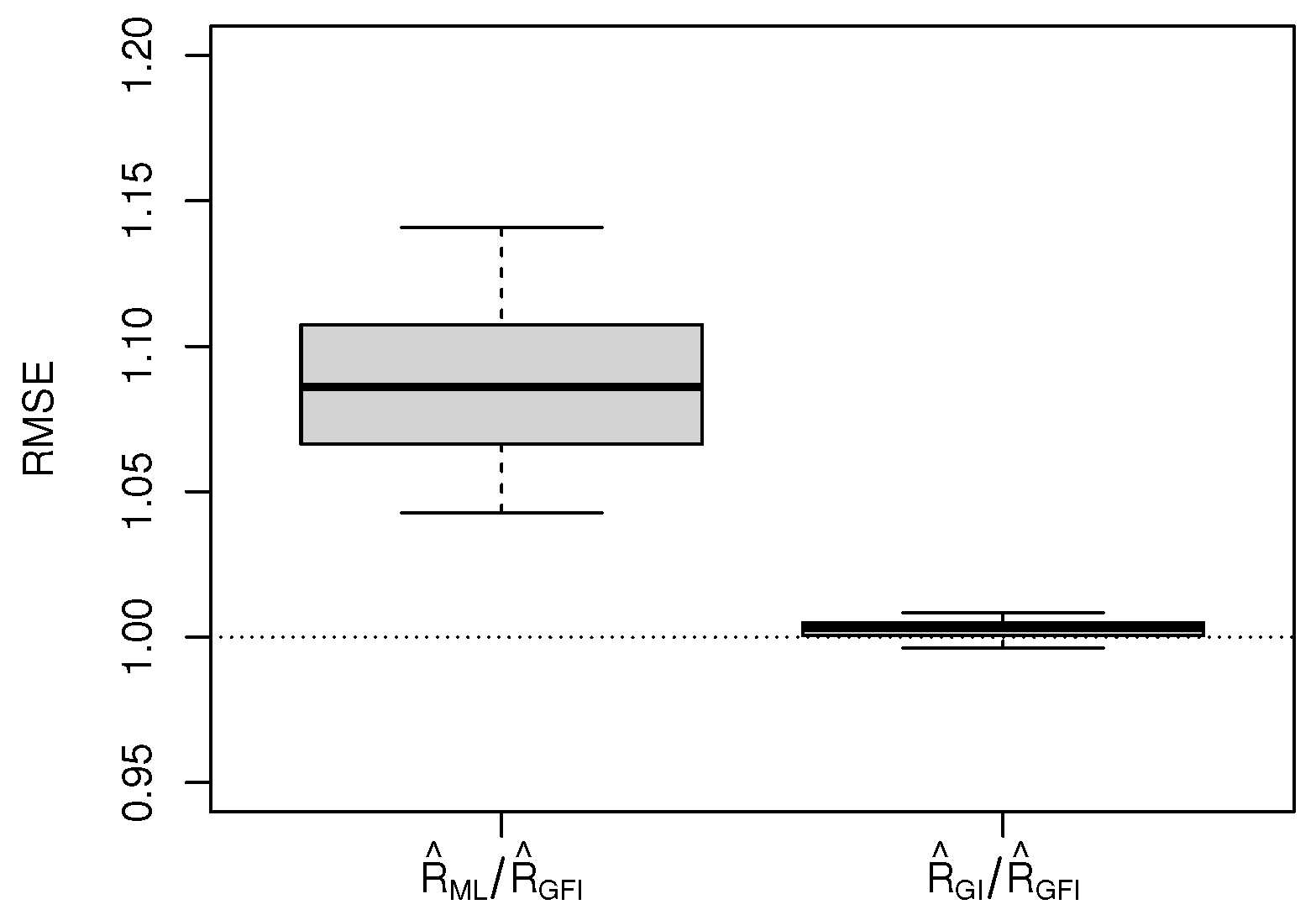
Table 1 provides the MSEs of
R for different parameter combinations, and
Figure 1 shows the boxplots of RMSEs of
R. The detailed information is shown as follows.
From
Table 1 and
Figure 1, the RMSEs of
are larger than 1 while the RMSEs of
are close to 1. Specifically, the MSEs of
are often smaller than those of
, and the gap is significant in small and moderate samples, such as
. Meanwhile, the difference between the MSEs of
and
is trivial.
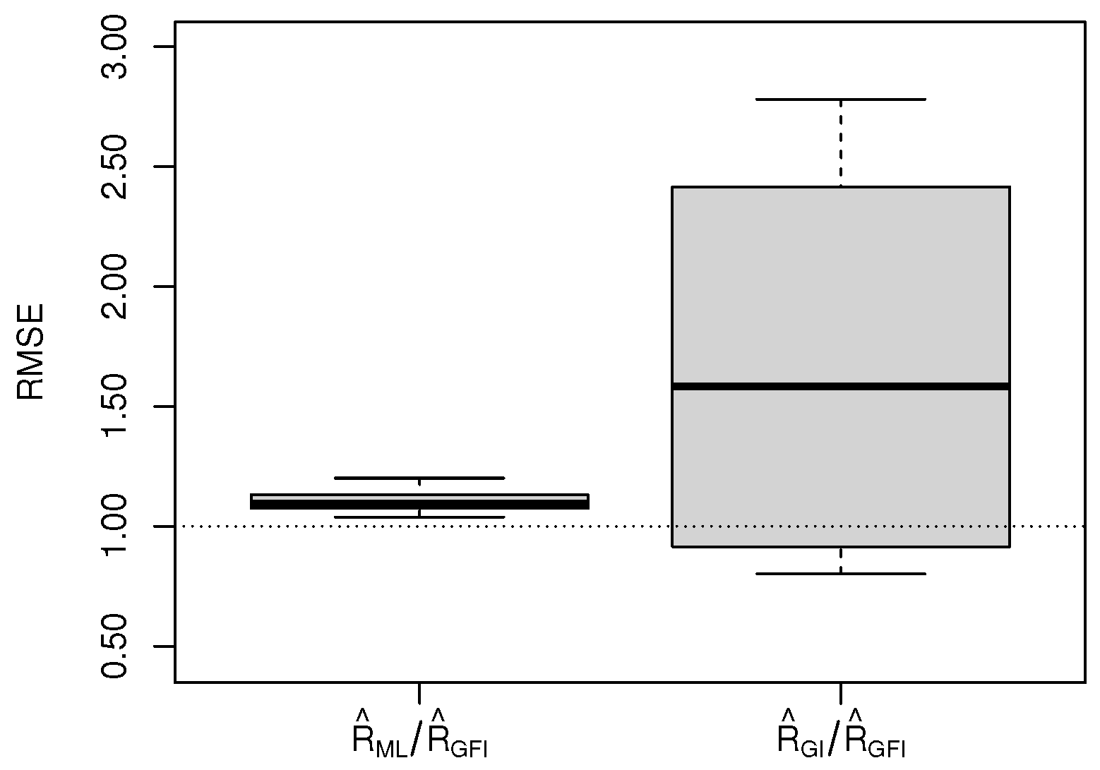
The MSEs of
R and the boxplots of RMSEs of
R under different parameter combinations are shown in
Table 2 and
Figure 2.
In
Figure 2, it is shown that the RMSEs of
and
are often larger than 1. From
Table 2, the MSEs of
are smaller than those of
, and the MSEs of
exhibit lower stability. At the same time, the MSEs of the three methods decrease with the increase in the sample size.
4.2. Analysis of Interval Estimates
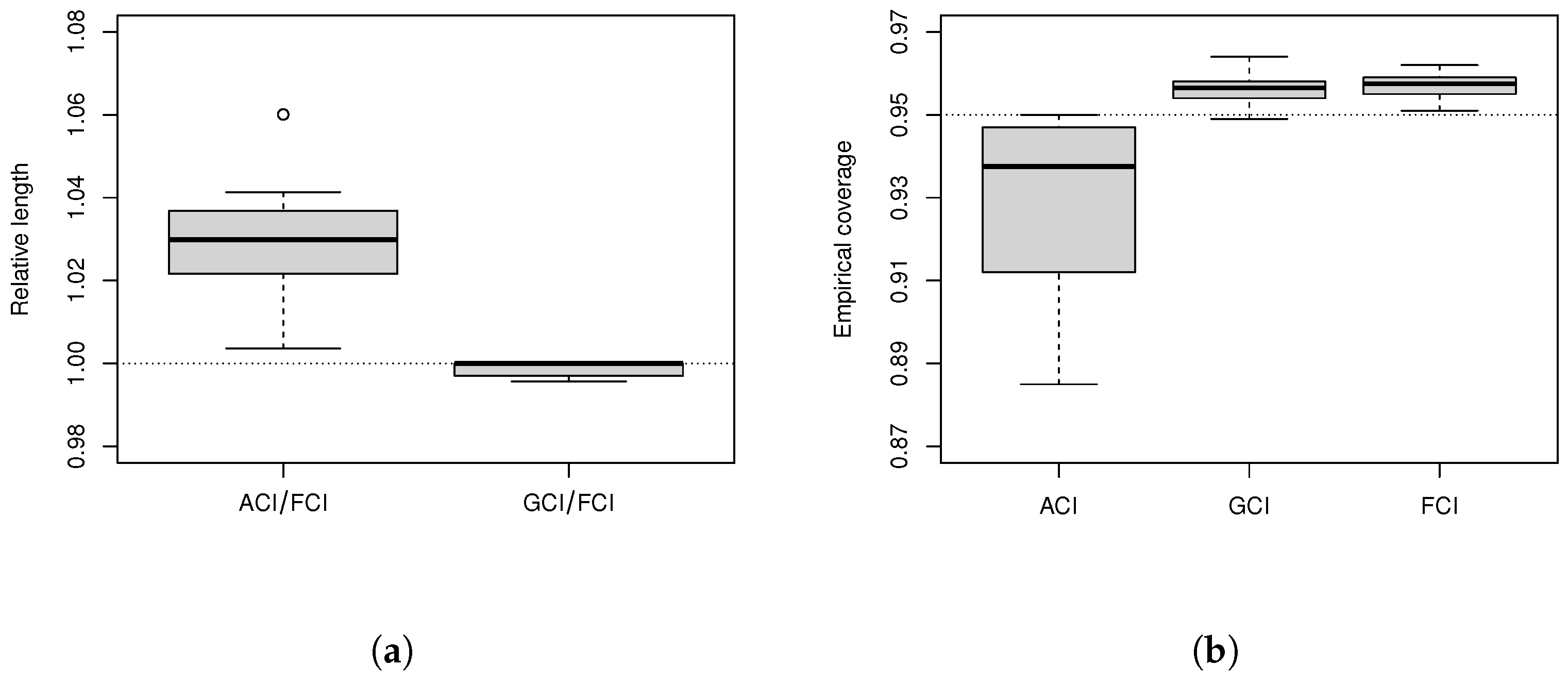
Table 3 provides the average length and empirical coverage of
R, and
Figure 3 shows the boxplots of relative length and empirical coverage. The details are as follows.
Table 3 and
Figure 3 show that the relative lengths of ACIs are greater than 1 and the ACIs are too liberal. The difference between GCIs and FCIs is small and both of them are conservative. When the sample size is small, GCIs and FCIs are better than ACIs. Meanwhile, the average lengths of the three methods tend to decrease with the increase in sample size.
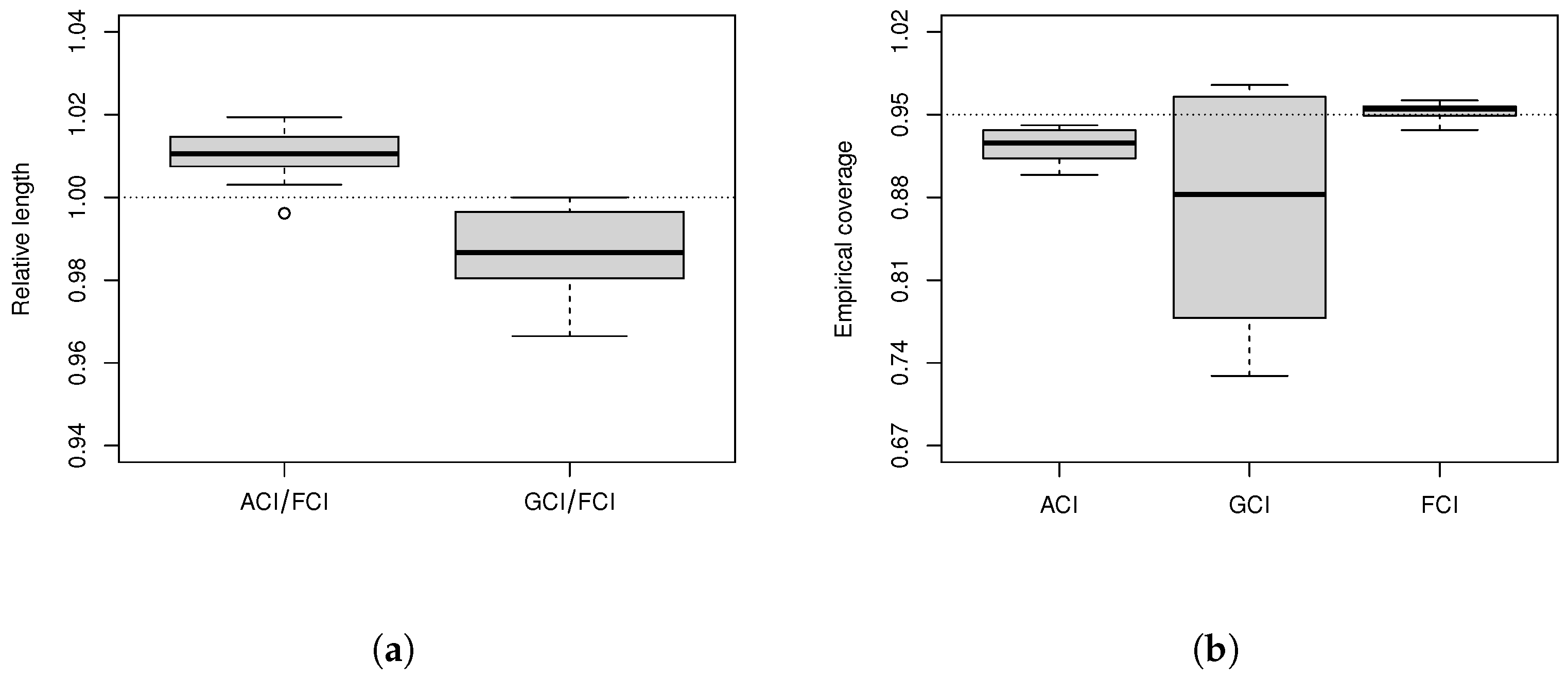
The average length and empirical coverage of
R, the boxplots of relative length, and empirical coverage are shown in
Table 4 and
Figure 4.
Figure 4 demonstrates that the relative lengths of ACIs are greater than 1 while those of GCIs are smaller than 1. FCIs are close to the nominal level while ACIs and GCIs are obviously liberal. To be specific,
Table 4 shows that the average lengths of ACIs are long while the empirical coverages of ACIs are often less than 0.95. The average lengths of GCIs are short, but the empirical coverages of GCIs exhibit instability. The average lengths of FCIs and GCIs are comparable when the sample size is large, and FCIs can reach the nominal level.
6. Discussion
The estimation of R in the GL distribution is an important research problem. Most of the existing literature studies focus on the ML estimation and Bayesian inference. However, the ML estimation cannot obtain the exact pivotal quantity and its empirical coverage sometimes fails to reach the nominal level. In Bayesian inference, the choice of the prior distribution is improper or subjective. Therefore, we introduce two novel methods to estimate R in the GL distribution.
On the one hand, there are two theoretical implications worth noting. First, the GFI method is applied to estimate R. The prior of the GFI is based on actual data, which makes the posterior distribution more objective. In addition, the weighted prior is applied when the scale parameters are the same. Our findings suggest that this approach of constructing the prior is suitable for estimating R in the two-parameter GL distribution and can be extended to other distributions as well. Second, the GI method offers another way when the conventional pivotal quantity is not available. By developing two lemmas, the generalized point estimation and generalized confident interval of R can be given.
On the other hand, this article has three practical implications. First, the simulation results indicate that the generalized fiducial method is better for the point estimation of R with the comparisons of the MSE. Moreover, it can be concluded that the GFI method often outperforms the ML and GI methods for the interval estimation of R, which presents more advantages in average length and empirical coverage. Second, the results of the three real data example state that the estimation of R can be applied in many different fields. Third, the two-parameter GL distribution without a location parameter is particularly useful in estimating R, where the dataset contains values less than zero. This characteristic expands its applicability to a wider range of datasets and deserves more attention in the scale-shape life distribution.
There are some limitations in our study. Due to encountering censored data in numerous survival analyses, such as the research of Rao [
39], Babayi and Khorram [
40], and Wang et al. [
41], the statistical inference of parameters, reliability, and stress–strength based on censored samples under the GL distribution would be an interesting direction for future works.


