Balancing Tradeoffs in Network Queue Management Problem via Forward–Backward Sweeping with Finite Checkpoints

Abstract

Network queue management can be modelled as an optimal control problem and is aimed at controlling the dropping rate, in which the state and control variables are the instantaneous queue length and the dropping rate, respectively. One way to solve it is by using an indirect method, namely forward–backward sweeping based on the Pontryagin minimum principle to derive control the trajectory of the dropping rate. However, there exists some performance balance issues in the network queue, such as memory usage versus runtime of the algorithm, or dropping rate versus network queue length. Many researchers have exploited symmetry for constrained systems, controllers, and model predictive control problems to achieve an exponential memory reduction and simple, intuitive optimal controllers. In this article, we introduce the integration of the checkpointing method into forward–backward sweeping to address such balancing issues. Specifically, we exploit the revolve algorithm in checkpointing and choose a finite number of checkpoints to reduce the complexity. Both numerical and simulation results in a popular network simulator (ns-2) are provided through two experiments: varying bandwidth and offered load, which solidify our proposal in comparison to other deployed queue management algorithms.

1. Introduction

Queue management problems with network devices has been an attractive research area in recent decades because of its strong impact on network performance in cases of congestion. Due to simplicity, DropTail is the current default queue management in most network routers and input/output (I/O) cards of personal computers, or it is integrated into the operating system’s kernel. It drops packets only when the buffer is fully occupied. Having been used for a long time with high link utilization, DropTail, however, has some weaknesses in terms of performance balancing that need to be addressed. Firstly, using DropTail, buffer size directly interacts with the performance of transport protocols and damages them in some rare cases [1]. A big excess buffer generates excessive queuing latency and poor recovery as a result of long retransmission time-outs. A limited buffer, on the other hand, can lead to low link utilization with frequent packet drops. DropTail as passive queue management might occur in bursts of packet drops, resulting in several packet drops from a single-traffic burst, irrespective of the buffer size. Secondly, DropTail might result in bad fairness and sharing among TCP connections [2]. Moreover, the queue length at a bottleneck point can extend high, especially when the buffer size is large, so that users at the receiver side might experience long delays. These reasons lead to the urgent need for deployed active queue management (AQM). Several approaches to model and derive an AQM algorithm include the additive-increase/multiplicative-decrease (AIMD) model of interaction between transport control protocol (TCP) and AQM [3], followed by using control theory or optimization tools to analyse bottleneck performance. Moreover, researchers established a memory reduction technique for the symmetric controllers [4]. Alternatively, a recent approach is to model the queue management problem of symmetrical differential equations using an optimal control approach and then solve it by the forward–backward sweeping method (FBSM) based on the Pontryagin minimum principle. In the first-order method based on gradient, FBSM is simple to implement and can run fast. Two sweeps are executed over the time interval: forward and backward (adjoint) sweeps. The basic idea is to implement FBSM straight forward and memorize all intermediate states in every sweep for state variable (queue length) and control variable (dropping rate). In addition, an AQM algorithm requires memory efficiency due to limited memory resources in network devices. In order to implement AQM with the indirect method, setting a finite number of checkpoints instead of storing all intermediate values is necessary; the checkpointing method has been addressed in the literature [5,6,7]. Briefly, checkpointing can provide us with memory efficiency by selecting only a finite checkpoint instead of storing all intermediate values; thus, solutions of OCQ as AQM are feasible. However, to reach memory efficiency, we sometimes have to sacrifice the other performance criterion. An example is the memory usage and runtime, which are two important requirements when implementing integrated algorithms into network devices’ firmware, e.g., Wi-Fi access points, mobile nodes, routers, etc, which own limited memory resources. In [5], the authors point out that higher memory usage is not equivalent to a higher runtime of an algorithm. An AQM algorithm should be lightweight, proactive and plain to implement in wired or mobile ad hoc networks [8,9]. Performance balancing of an AQM algorithm should be reached as well, i.e., the balance between performance criteria results. Within the current literature can be found some trade-offs, for instance, between queue length and packet drop rate. Higher drop rate results in shorter queue length. We want a short queue length, or a short delay experience for users, but “why do we should drop good packets” [10]. An algorithm that brings a good balanced result between such performance criteria is desirable. In this paper, we investigate the performance trade-off between different AQM disciplines and derive a novel AQM that has a good performance balance when compared to others. Optimal control has been exploited to investigate queue performance in computer networks in [11,12]. We analyze the FBSM-AQM algorithm with and without the use of the adoption of checkpointing. By integrating checkpointing into FBSM-AQM, the numerical and simulation results demonstrate that we can efficiently reduce memory usage by reasonable choosing the number of checkpoints, therefore making it easier for implementation. Our contributions are summarized as follows:

• From the Optimal Control Queue model (OCQ) of a network queue, with the objective of minimizing a weighted cost function of queue length and drop rate, we propose to solve it using an indirect method and derive a Forward–Backward Sweeping Method FBSM-AQM scheme (Section 3.1 and Section 5).
• We extend this method with checkpointing (FBSM-AQM-CP), which can deal with the trade-off between the memory usage and runtime of an algorithm by choosing a finite checkpoint (Section 6).
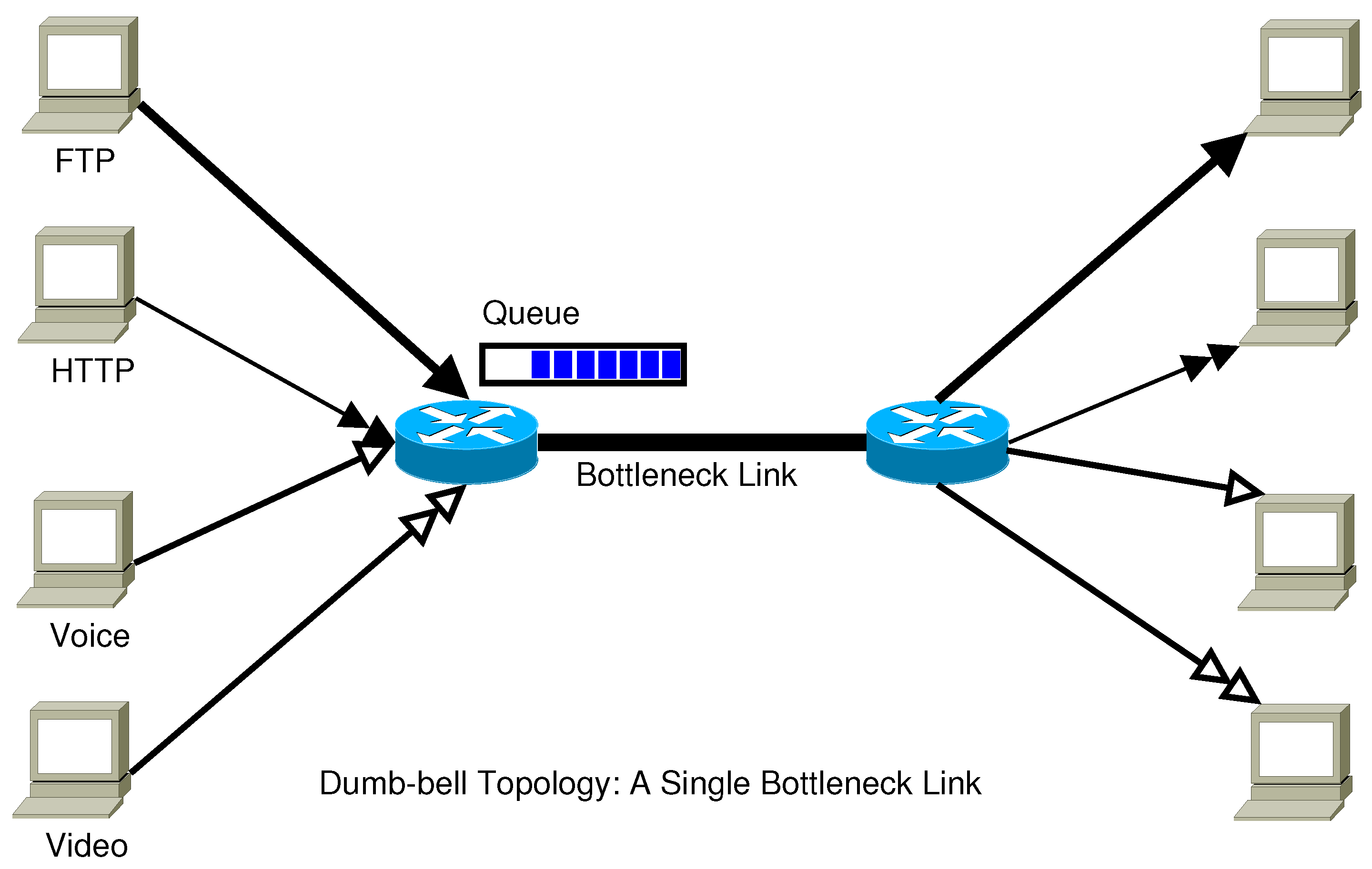
• We conduct and provide numerical and simulation results (ns2) to evaluate the proposed method FBSM-AQM-CP under dumb-bell network topology. We then suggest for designers a choice for the number of checkpoints to balance performance in Section 7.1 and Section 7.3.
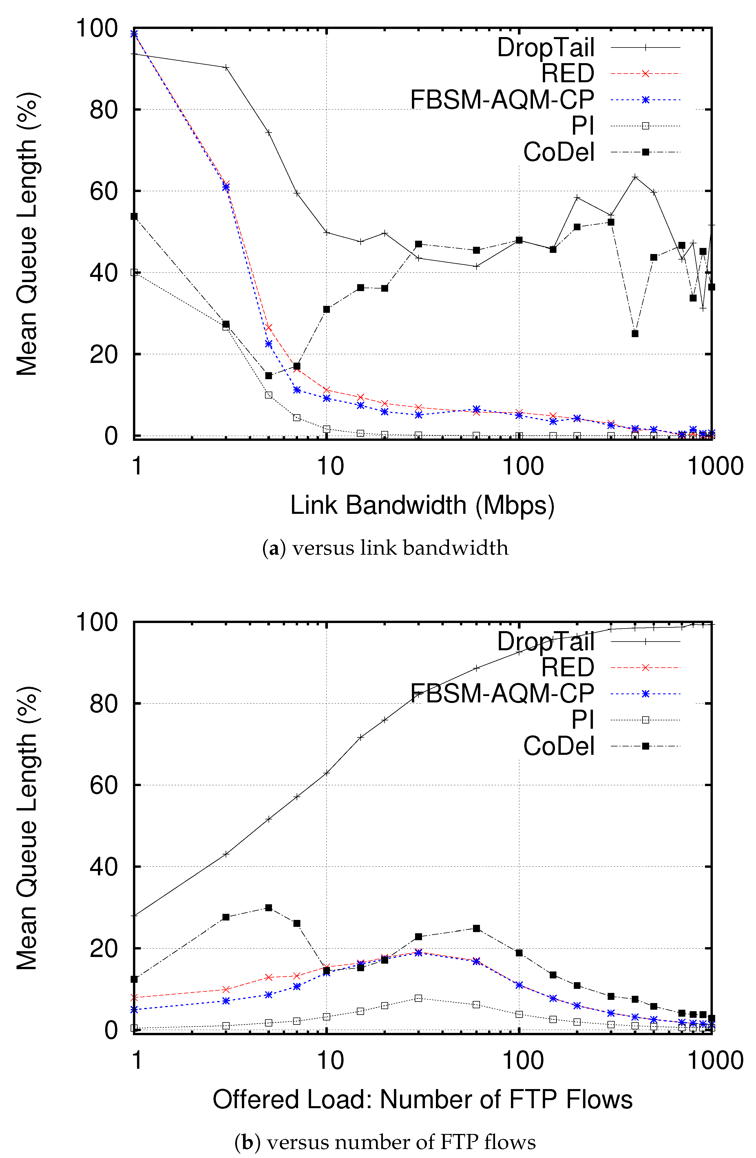
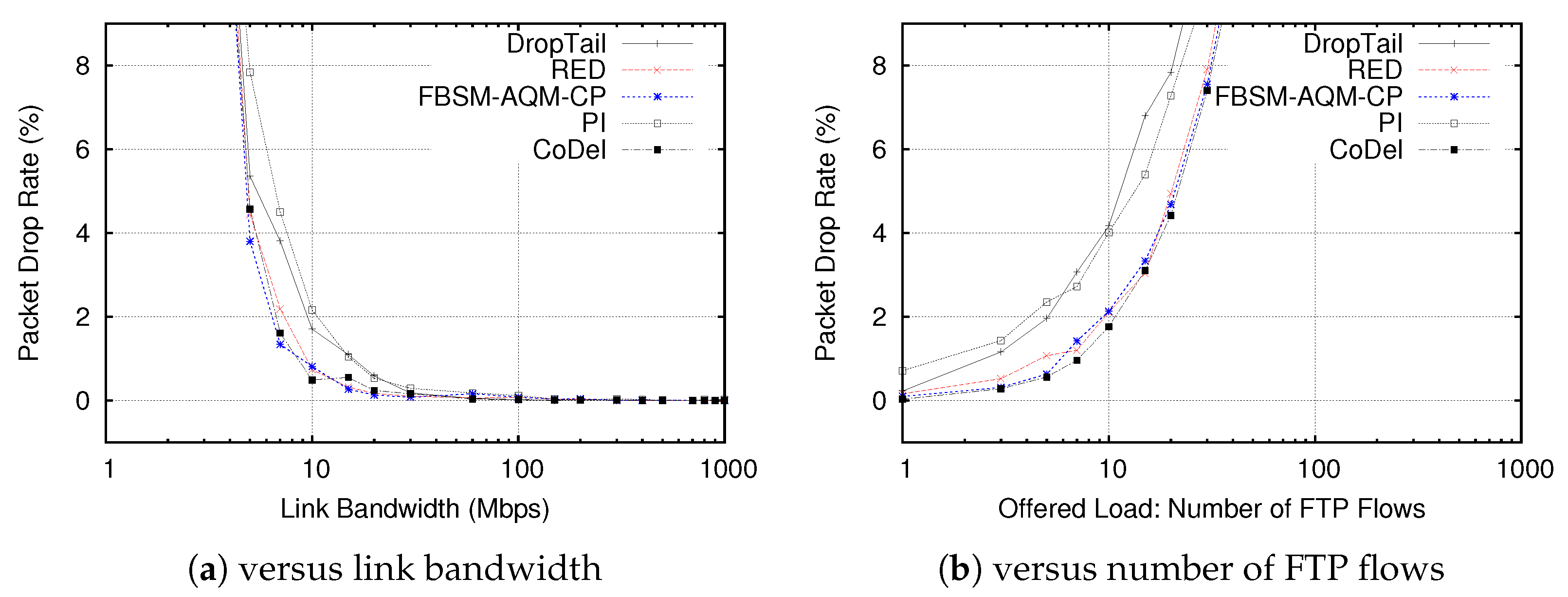
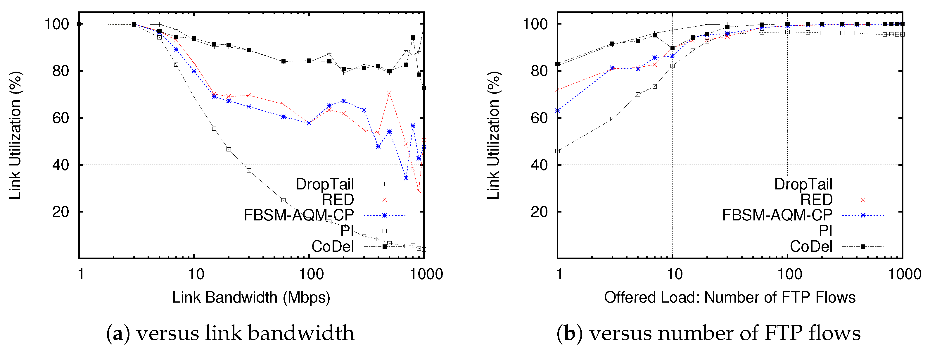
• The simulation results in Section 7.3 give some insights into the performance of our proposed AQM scheme and the others to be compared: queue length, packet drop rate and link utilization.

2. Related Works

In order to handle such an AQM scheme, common methods are based on the linearization of the TCP core model with control theory from Hollot et al. [3] and consist of random early detection (RED) [13], and proportional integral derivative (PID) [14] and contribute a large portion to the queue management field [15]. The primary objectives were to propose more specific design guidelines to improve stability and responsiveness; moreover, the behaviour of RED under a change in network circumstances, namely link bandwidth capacity, is more understandable. Using control theory, one can classify them into three different types of control: classical, fuzzy logic, and robust. Using feedback control, traditional PID controller-based algorithms have been developed as other AQM methods to fulfil certain internet criteria. Hollot et al. [3] investigated RED as an I-controller and suggested two options for improving RED, the proportional (P) and the proportional integral (PI) controllers. The Routh stability test is used to identify the stable zone of the control gain for dynamic-RED (DRED), with a load-dependent probability of ignoring packets at random once a buffer gets congested. It keeps the average queue size near to a predefined limit while allowing transient traffic bursts to be queued and while avoiding unessential packet drops. Its primary benefit is that there is no need to gather state data for individual flows. A robust control approach was also investigated in order to improve classical control. The DC-AQM algorithm, which is based on the internal mode compensation (IMC) principle, was used to address the issue of large delay with a large buffer in a bufferbloat [16]. They aimed to reduce latency by tuning the classical PID controller parameters $K_p$, $K_i$, and $K_d$ using the derived IMC controller. To deal with the high delay, a Gain Adaptive Smith Predictor with a PI controller (GAS-PI) in [17] was designed to enhance robustness. Thus, in [18], a predictive PID controller is suggested for TCP/AQM. They employed the generalized predictive control method to find appropriate values for $K_p$, $K_i$ and $K_d$, making the system more robust to changes in model parameters like offered load, round-trip time, etc. Fuzzy Control RED (FCRED) was suggested in [19]. It is made up of a fuzzy controller, adjusting the $P_{max}$ parameter of the RED algorithm. The fuzzy controller is made up of three parts: the fuzzification unit, a fuzzy-interference engine with fuzzy-rule base, and a de-fuzzification unit. The fuzzification module converts the controllable input values into a fuzzy set (i.e., membership functions). The fuzzy base is responsible for connecting the incoming signals to the proper outcome variable. Fuzzy logic rules can be created by trial and error—requiring the knowledge and expertise of an expert in the field of TCP congestion control— and they are sometimes not distributed and are hard to implement. Recently, new promising AQM schemes have been proposed to improve network performance balancing. An interesting commonality in their designs is that they are lightweight and easy to implement. In [20], they established a Proportional Integral controller Enhanced (PIE) controller as a lightweight AQM that did not require per-packet extra processing. Hence, small overhead could be achieved, and the algorithm was simple to implement in both hardware and software. In [21], Controlled Delay (CoDel) tackled the bufferbloat issue by directly controlling delay instead of queue length, as other AQMs do. Cascade Probability Control (CPC) is the most recent other method that we have developed for reducing queueing delay in wired networks [22]. To determine the delay stable interval of the transportation network, the authors in [23] exploited the nonlinear dynamics of TCP/AQM.

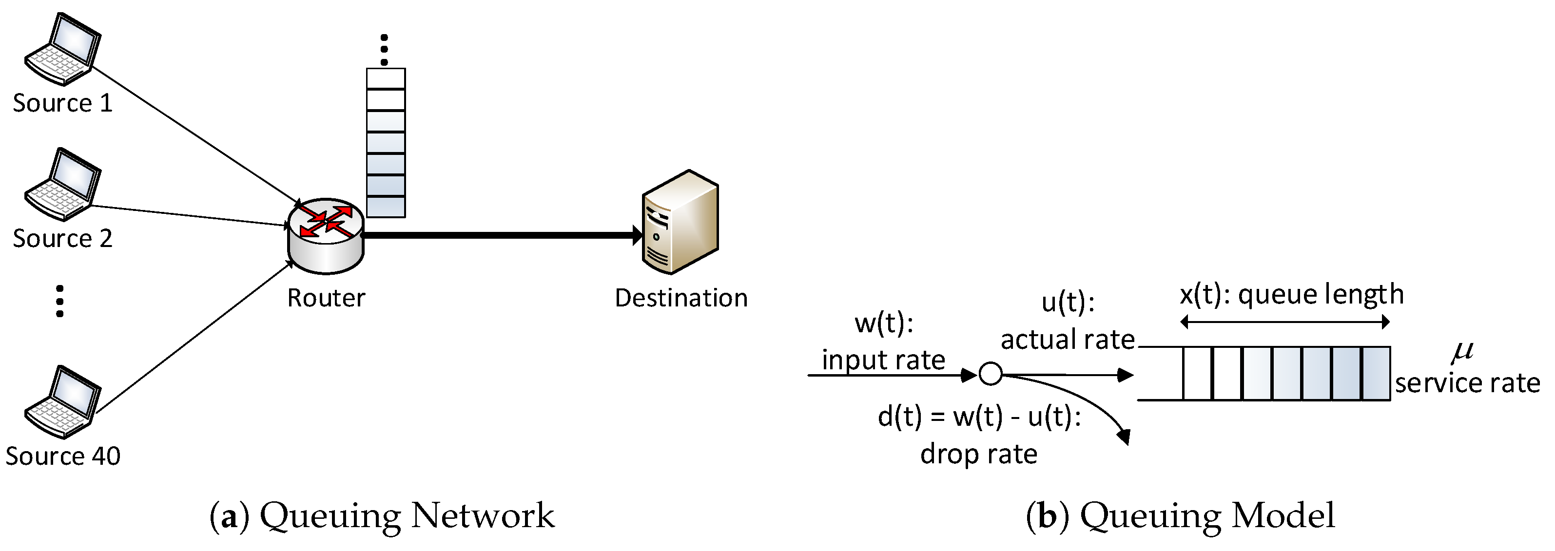
3. Model Description of Optimal Control Queue Model

The following dynamical system is the result of the mathematical formulation of the model that includes control dropping rate

$$\dot{x}\left(t\right)=f(x\left(t\right),u\left(t\right),t)$$

(1)

with initial condition $x(t=0)=x_0$. The model’s flow diagram is shown in Figure (Figure 1b), while the dynamical system’s inputs are listed in

Table 1. Entries of Model (1).

Notation	Description	Role
a	parameter for different type of queueing model;	Constant
	here, $a=1$, for the sake of simplicity,
	to model an M/M/1 queue.
$\mu$	service rate (bandwidth capacity);	Constant
u	dropping rate	Control variable
x	queue length	State variable

. Consider the system represented in Figure 1, which shows a standard network buffer layout. The model’s flow diagram is shown in (Figure 1b), while the dynamical system’s inputs are listed in Table 1. Consider the system represented in Figure 1b, which shows a standard network buffer layout. A certain number of packets arrive into the system every second in this scenario. In accordance with the number of packets $x\left(t\right)$ existing in the buffer and the network service rate $\mu$, it might be advantageous to drop a portion of this forthcoming flow. The dynamic system of the buffer load is represented by Equation (1). In order to minimize the cost functional, control variable $u\left(t\right)$ should be chosen, which creates a balance between dropping rate and queue length. The following objective can be used to express this purpose mathematically:

$$\underset{0\le u\left(t\right)\le w}{min}{\int }_{t=0}^{t_f}x\left(t\right)+R(w-u\left(t\right))$$

(2)

where $R,w$ stand for weight on dropping rate and input rate, respectively.

3.1. Characterization of Optimal Control

According to Pontryagin’s minimum principle PMP [24], it can be used to solve the problem of restricted dynamical optimization of queuing network (2) subject to (1) (named Figure 1b in [25]). To get started, we will need to define the Hamiltonian function:

$$H(\psi \left(t\right),x\left(t\right),u\left(t\right))=x\left(t\right)+R(w\left(t\right)-u\left(t\right))+\psi \left(t\right)(u\left(t\right)-\frac{\mu x\left(t\right)}{a+x\left(t\right)})$$

(3)

where $\psi \left(t\right)$ denotes the adjoint function that satisfies:

$$\dot{\psi }\left(t\right)=-H_x(\psi \left(t\right),x\left(t\right),u\left(t\right)),\psi \left(t_f\right)=0$$

(4)

When the constraint is relaxed by one unit, the objective function computed on the optimal solution changes.

Proposition 1.

Given an optimal control $u^{*}\left(t\right)$ and its corresponding state trajectory $x^{*}\left(t\right)$ of the system (1), then there exists an adjoint function $\psi \left(t\right):[0,t_f]\to R$ satisfying

$$\dot{\psi }\left(t\right)=-1+\psi \left(t\right)\frac{a\mu }{{(a+x\left(t\right))}^2},$$

(5)

furthermore,

$$u^{*}\left(t\right)=arg\underset{0\le u\left(t\right)\le w}{min}H({\psi }^{*},x^{*},u)$$

(6)

Proof. 

The adjoint equation with transversality condition (5) is standard for PMP, which establishes the necessary condition for the optimality of $u^{*}\left(t\right)$. Because the control is bounded, these necessary optimality requirements can be written in the following way [24]:

$$u^{*}\left(t\right)=\left\{\begin{array}{cc}0\hfill & \mathrm{if}{H}_u\ge 0\hfill \\ u_{sing}\hfill & \mathrm{if}{H}_u=0\hfill \\ w\hfill & \mathrm{if}{H}_u\le 0\hfill \end{array}\right.$$

Since H does not depend on u, PMP gives no information about $u^{*}$ when $H_u=0$. A fluid flow buffer’s optimal control is a class of bang-bang control with a potential of singular arc $[t1,t2]$:

$$\frac{d^{\left(i\right)}}{d{t}^{\left(i\right)}}\left[H_u\right]=0,\forall i\in N,\forall t\in [t_1,t_2]$$

$$\frac{d}{dt}\left[H_u\right]=\dot{\psi }=-1+\psi \left(t\right)\frac{a\mu }{{(a+x\left(t\right))}^2}$$

At $\psi =R$, then $x^{*}=\sqrt{aR\mu }-a$. The second derivative of $H_u$ with respect to the t is then

$$\frac{d^2}{d{t}^2}\left[H_u\right]=\dot{\psi }\frac{a\mu }{{(a+x\left(t\right))}^2}+\psi \frac{-2a\mu }{{(a+x\left(t\right))}^3}\dot{x}=0$$

then,

$$u_{sing}=\mu (1-\sqrt{\frac{a}{R\mu }})$$

In a more unified and symmetric way, we can get the optimal control $u^{*}\left(t\right)$:

$$u^{*}\left(t\right)=\left\{\begin{array}{cc}0\hfill & \mathrm{if}{H}_u\ge 0\hfill \\ \mu (1-\sqrt{\frac{a}{R\mu }})\hfill & \mathrm{if}{H}_u=0\hfill \\ w\hfill & \mathrm{if}{H}_u\le 0\hfill \end{array}\right.$$

   □

To tackle the problem ((1) and (2)), we present a forward–backward sweeping technique (FBSM) with two sweeps based on an indirect approach in optimal control. A control trajectory of control variable $u\left(t\right)$ (dropping rate in queue) can be produced as an output after numerically solving it with the FBSM [26,27] Using this control trajectory, an algorithm for active queue management, namely FBSM-AQM (1), is able to be implemented in network simulation ns2 by modifying the dropping function. Here, we detail the procedure we use to solve the problem of optimal control queue (OCQ) and propose our algorithm using an indirect method from optimal control theory.

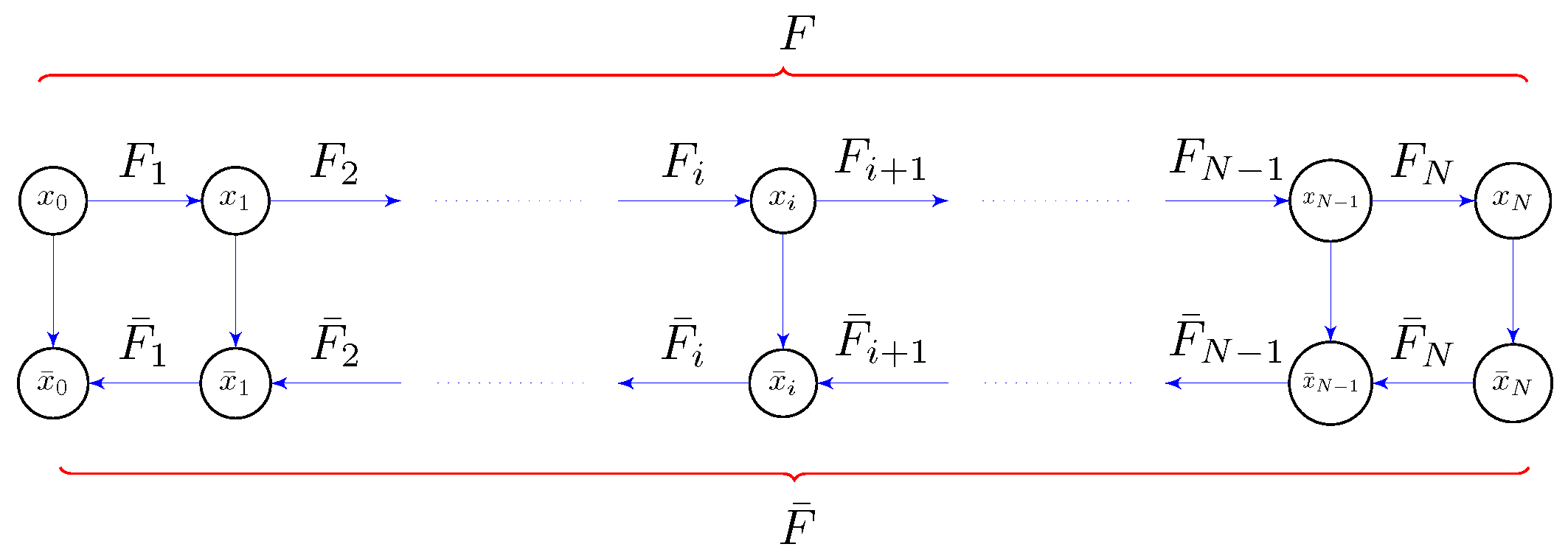
4. Forward–Backward Sweeping Method (FBSM)

Since U and H are convex, the control function can be computed in a particular way for each t. We introduce the symmetric problem of minimizing the Hamiltonian with regard to the control u:

$$\underset{u\in U}{min}H(\psi ,x,u)\forall t\in [t_0,t_f]$$

Optimal control u is usually written explicitly as a function of the trajectory, adjoint, and times as $u=u(\psi ,x,t)$. And after insertion it into the system, a boundary value problem (BVP) is derived. We linearise around the solution $u\left(t\right)$ and get the variation equation of $u\left(t\right)$ as:

$$0={H_u}^{\top }+H_{uu}\delta u\left(t\right)$$

(7)

Equation (7) can be approximated using Strong Legendre-Clebsch condition as:

$$\delta u\left(t\right)=arg\underset{\delta u\in \{U-u\}}{min}{H}_{aug}(\psi ,x,u+\delta u,t)$$

(8)

Here, $H_{aug}=H(\psi ,x,u+\delta u,t)+\beta {\Vert \delta u\Vert }^2$ represents the augmented Hamiltonian function. In order to calculate the control iteratively using Equation (8), a parametric optimization technique has been proven to be an efficient way [27]. If $\beta =0$, the set U is convex, and the function H is convex with regard to the control u, then $\delta u$ is a descent direction. In case of an absence of the reduction of the objective, we try different $\beta$ until the reduction is satisfied. The indirect approach motivates us to design FBSM-AQM Algorithm 1 [26,27].

Algorithm 1 FBSM-AQM.

1: Initialization:     $u_{\mathrm{new}}\left(t\right)=u\left(t\right),\delta u\left(t\right),\forall t\in [t_0,t_f];$     ${\mathcal{J}}_{\mathrm{old}}=\infty ,\gamma =0,\beta ,\rho \in (0,1);$     $\mathrm{Step}=1,\mathrm{MaxStep},ϵ$. 2: while$\mathrm{Step}\le \mathrm{MaxStep}$do 3:     procedure Integrate Forward 4:         $x_{\mathrm{new}}\left(t_0\right)=x_0,{\mathcal{J}}_{\mathrm{new}}\left(t_0\right)=0.$ 5:         $\mathbf{Sweep}\mathbf{1}:t:t_0\to t_f$ 6:         if $\mathrm{Step}>1$ then 7:            $\delta u\left(t\right)=arg\underset{\delta u}{min}{H}_{aug}(x\left(t\right),u\left(t\right)+\delta u,\psi \left(t\right),t);$ 8:            $u_{\mathrm{new}}\left(t\right)=u\left(t\right)+\delta u\left(t\right).$ 9:         end if 10:         ${\dot{x}}_{\mathrm{new}}\left(t\right)=f(x_{\mathrm{new}}\left(t\right),u_{\mathrm{new}}\left(t\right),t).$ 11:         $\dot{{\mathcal{J}}_{\mathrm{new}}}\left(t\right)=l(x_{\mathrm{new}}\left(t\right),u_{\mathrm{new}}\left(t\right),t).$ 12:     end procedure 13:     ${\mathcal{J}}_{\mathrm{new}}={\mathcal{J}}_{\mathrm{new}}\left(t_f\right).$ 14:     if ${\mathcal{J}}_{\mathrm{new}}<{\mathcal{J}}_{\mathrm{old}}$ then 15:         ${\mathcal{J}}_{\mathrm{old}}={\mathcal{J}}_{\mathrm{new}},\beta =\beta \rho .$ 16:     else 17:         $\beta =\beta /\rho ;\mathrm{go}\mathrm{to}\mathrm{Integrate}\mathrm{Forward}$ 18:     end if 19:     procedure backward Sweep 20:         $\psi \left(t_f\right)=0,\gamma \left(t_0\right)=0.$ 21:         $\mathbf{Sweep}\mathbf{2}:t:t_f\to t_0.$ 22:         $x\left(t\right)=x_{\mathrm{new}}\left(t\right),u\left(t\right)=u_{\mathrm{new}}\left(t\right).$ 23:         $\dot{\psi }{\left(t\right)}^{\top }=-\frac{\partial H\left(\psi \right(t),x(t),u(t),t)}{\partial x}$ 24:         $\overline{u}\left(t\right)=\frac{\partial H\left(\psi \right(t),x(t),u(t),t)}{\partial u}.$ 25:         $\dot{\gamma }\left(t\right)={\Vert \overline{u}\left(t\right)\Vert }^2.$ 26:         $\gamma =\gamma \left(t_f\right).$ 27:     end procedure 28:     if $\parallel \gamma \parallel <ϵ$ then 29:         $\mathrm{terminate};$ 30:     end if 31:     $\mathrm{Step}\leftarrow \mathrm{Step}+1.$ 32: end while

5. FBSM-AQM without Checkpointing

FBSM Algorithm 1 is made up of two sweeps over the time interval $[t_0,t_f]$ forward and adjoint sweeps, respectively. The adjoint integration has to be executed backward in time, and the entire forward trajectory $x=(x_0,\cdots ,x_{N-1})$ is required. A specific sequence of intermediate states is to be calculated through the evaluation of a forward simulation F. The FBSM Algorithm 1 is made up of two forward and adjoint sweeps through the time interval $[t_0,t_f]$, respectively. The adjoint integration must be conducted backwards in time, and the entire forward trajectory $x=(x_0,\cdots ,x_{N-1})$ must be completed. During the computation of a forward simulation F, it is necessary to compute a specific sequence of intermediate states. Each transition from one intermediate state to the next is a time step. $F_i$ (see Figure 2). As a result, we could claim that the computation of a particular forward simulation F may be described as a calculation of N time intervals $F_i(x_{i-1},u_{i-1},t_{i-1})$, $1\le i\le N$(as shown in Figure 2). If the time step $F_i$ is applied to the preceding state $x_{i-1}$, the intermediate state $x_i$ could be computed. Based upon only the date from the preceding state $x_{i-1}$, the time step $F_i(x_{i-1},u_{i-1},t_{i-1})$ computes the intermediate state $x_i$. For the adjoint integration, one may use ${\psi }_{i-1}={\overline{F}}_i({\psi }_i,x_{i-1},u_{i-1},t_{i-1})$ motivated by the adjoint equation that belongs to the differential equation depicting the state. This forward simulation F must be reversed (as seen in Figure 2) if one solves the adjoint problem affiliated with a presumed forward simulation F.

The basic scheme [5,7] is the simplest approach for implementing FBSM Algorithm 1, storing all intermediate states of each sweep and restoring them when needed. The amount of memory required for the method is commensurate to the number N of time steps in a forward simulation F (see Algorithm 2). As a result, it has the potential to be enormous. This strategy, on the other hand, can only be satisfied if there is enough memory available.

Algorithm 2 FBSM-AQM-NoCP.

1: $\mathbf{Computing}\&\mathbf{Recording}\mathbf{:}\mathrm{Set}x\mathrm{to}\mathrm{the}\mathrm{initial}\mathrm{value}{x}_0$ 2: while$i=0,N-1,1$do 3:     $\mathrm{Execute}{x}_{i+1}=F_i(x_{i-1},u_{i-1},t_{i-1})$ 4: end while 5: $\mathrm{Returning}\text{:}\mathrm{Set}\psi \mathrm{to}\mathrm{the}\mathrm{terminate}\mathrm{value}{\psi }_N$ 6: while$i=N,1,-1$do 7:     $\mathrm{Execute}{\psi }_{i-1}={\overline{F}}_i({\psi }_i,x_{i-1},u_{i-1},t_{i-1})$ 8: end while

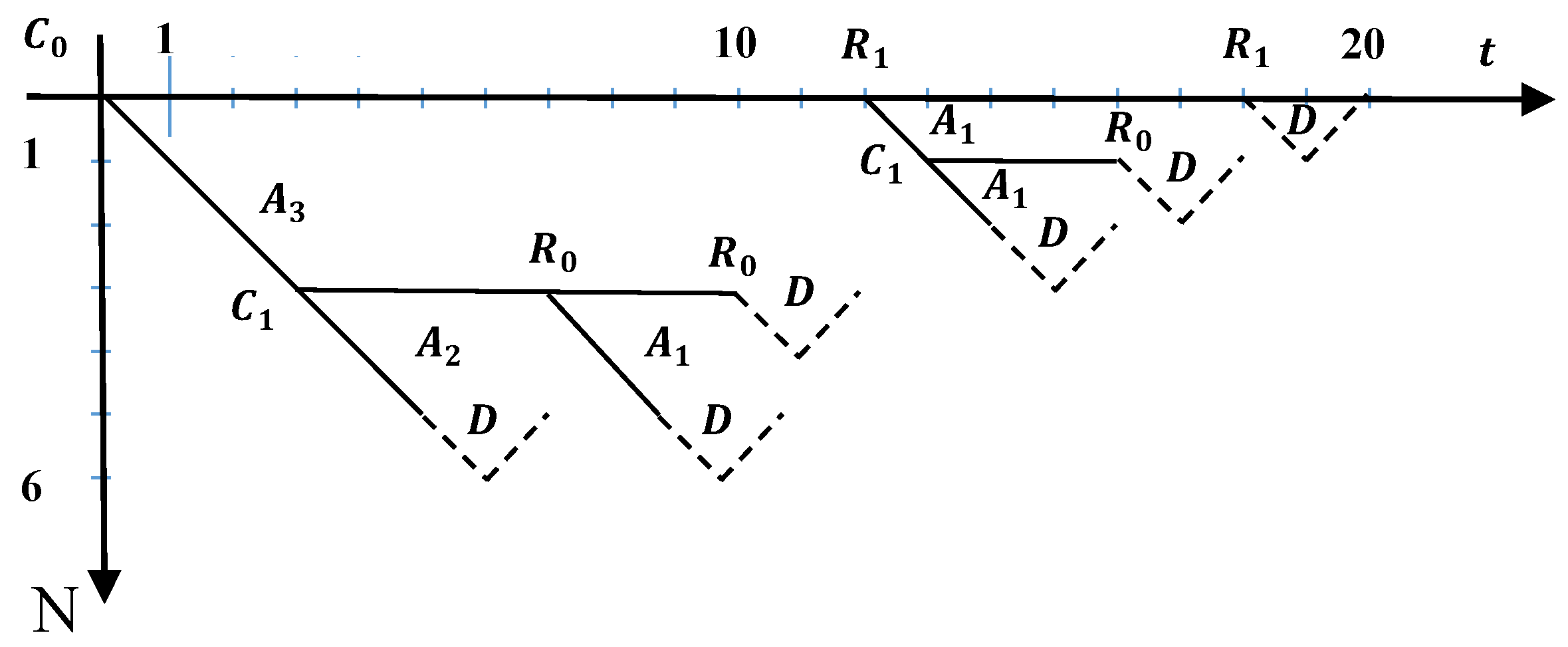
6. FBSM-AQM with Checkpointing

A different method for reversing a forward simulation F does not necessitate memorizing all intermediate states, but only a subset of them. Memorized intermediate states are known as checkpoints. Thus, the approach is known as checkpointing [5,7,27,28]. We can only memorize a small number of intermediate states at a time, depending on available memory capacity. As a result, this method drastically minimizes the amount of memory required. The computation of some intermediate trajectories at some time intervals may run numerous times through the reversal of a forward simulation F. As a result, the evaluation procedure must be conducted several times. A forward simulation F does not need to be restarted from the primary intermediate state. A proper checkpoint can be used to relaunch it.

Definition 1

(Reversal Schedule $\mathbf{S}$ [5]). Assume a forward sweep F with N time intervals $F_i,1\le i\le N$. Let $c\in \mathbb{I}$ checkpoints be accessible, each of which can accommodate the data of an elementary intermediate state. N represents the current final time step, j represents the number of memorized checkpoints, and i represents the current state. Initially, $i=i_0\ge 0,j=j_0\ge 0$, and $i<N\le \infty$. With $q\ge 1$ and starting with $N\ge 1,i=0$. Thus, a reversal schedule S is made up of a bounded sequence of the next operations:

• Advance operation $A_k$= make forward computations by increment i by $k\in [1,N-i-1]$;
• Takeshot operation $C_j$= memorize state i to checkpoint $j\in [1,q]$;
• Restore operation $R_j$= reset i to checkpoint $j\in [1,q]$;
• Firs-turn and youturn operations D= do the first reversal step if $i=N$ and one reversal step by decrement N by 1 if $i=N-1$, respectively.
  Up to N has been reduced to zero.

Every schedule defined in this way for a given combination $(N,c)$ is known to be admissible. We suppose that each admissible reversal S starts with the operation $C_0$, which reads an initial intermediate state from the checkpoint $j_0$, without loss of generality. The operation A is represented by $A_k$ if it is repeated up to k times. For example, let $N=6$ and $c=2$ be given. The time intervals $Fi$ are plotted vertically on the y-axis, while the time necessary to evaluate single operations is plotted horizontally on the x-axis The time is measured in w-units. Because the initial checkpoint includes data from the intermediate state $x_0$ and is located on it, the computational axis represents a checkpoint. The following describes the evaluation of the reversal schedule S as depicted in Figure 3: Firstly, the operation $C_0$ is executed, i.e., the first checkpoints $j_0=0$ are used to read out the initial intermediate state $x_0$. Following that, the three time intervals $F_1$, $F_2$, and $F_3$ are evaluated in order, as described by the operation $A_3$. The operation $C_1$ then saves the intermediate state $x_3$ into the first checkpoint. The action $A_2$ performs the following two time intervals $F_4$ and $F_5$ in a sequential order. Operation D is then executed for the first time, allowing the adjoint step $\overline{F_6}$ to be assessed. Then, using operation $R_0$, data from the intermediate state $x_3$ is read out of the first checkpoints. Procedure $A_1$ evaluates the time step $F_4$ using this data. Using operation D, it is now able to do the adjoint step $\overline{F_5}$. Following that, a similar idea is repeated multiple times up until all adjoint steps $\overline{F_1},\cdots ,\overline{F_6}$ are completed in order. Furthermore, memory is in demand for the storing of data generated throughout a single time step $F_i,1\le i\le 6$, as well as for the execution of a corresponding adjoint step $\overline{F_i},1\le i\le 6$. Consider the operator ≻ that orders the evaluation in such a way that the left hand one is realized before the right hand one. Now, the reversal schedule S of the example can be represented by:

$$\begin{array}{ccc}\hfill S& =& C_0\succ A_3\succ C_1\succ A_2\succ D\succ R_0\succ A_1\succ D\succ R_0\succ \hfill \\ & & D\succ R_1\succ A_1\succ C_1\succ A_1\succ D\succ R_0\succ D\succ R_1\succ D.\hfill \end{array}$$

It can be executed using $20w$ units requiring only the memory of 2 checkpoints. Memory is required to store the data generated over each time step $F_i$ to calculate the matching adjoint step. If Algorithm 2 is applied, $12w$ units are required to carry out six adjoint steps $\overline{F_i},1\le i\le 6$; however, all intermediate states $x_i,1\le i\le 6$, in addition to the data produced over all single time intervals $F_i,1\le i\le 6$, that is needed for the implementation of corresponding adjoint steps $\overline{F_i},1\le i\le 6$, will be memorized. The main issue is deciding where to place the checkpoint (c). Let $\varsigma (c,t)$ denote the maximum length, i.e., the maximum number of time intervals, of any computational chain that can be reversed with a maximum of c checkpoints and a maximum of t forward steps from any of the states. Then, Griewank [6,7] shows that $\varsigma (c,t)=\left(\genfrac{}{}{0pt}{}{c+t}{c}\right)$, and with this equality, the memory requirement and the number of operations have a logarithmic dependence on the runtime of the function evaluation. If the values of the first two quantities are known, the third quantity can be calculated. Specifically, the maximum number of steps, checkpoints, and repeated forward steps can be found without recording of intermediate. For instance, if there are 6 time intervals, and three checkpoints can be stored, $t=2$ is obtained. After the initial one at zero, the value of $\varsigma (c,t-1)$ (here $\varsigma (2,1)=3$) determines the next checkpoint. As a result, state 3 is marked as checkpointed, as shown in Figure 3.

7. Performance Evaluation and Discussion

7.1. Tradeoff: Runtime & Memory Usage

In this portion, we measure the runtime of the suggested algorithms. We choose the time-step of 1000 and vary the number of checkpoints to check the performance of FBSM-AQM when and when not applying checkpointing. Firstly, without the checkpointing method and a large time-step, the algorithm might not run and display some errors, i.e., segmentation fault (core dumped). But if we use the checkpointing method and vary the number of checkpoints from 10 to 1000, the algorithm can run at different rates or runtimes. In Figure 4, let us define the ratio of runtime as the ratio between the runtime needed by the reversal schedule and the straight forward approach (Algorithm 2). From that definition, we describe it as the following:

$$\mathrm{ratio-run-time}=\frac{\mathrm{RunTime}\left(\mathrm{FBSM-AQM-CP}\right)}{\mathrm{RunTime}\left(\mathrm{FBSM-AQM-NoCP}\right)}.$$

(9)

For instance, in Figure 4, when the number of checkpoints is equal to ≈40, the ratio runtime is ≈2. It implies that the runtime required by algorithm FBSM-AQM-CP is twice as much as the runtime required by algorithm FBSM-AQM-NoCP. When we increase the number of checkpoints up to 500, the ratio runtime is approximately equal to 1, which implies the runtime of the algorithm using checkpoint is reduced as the number of checkpoints is increased. The stage at which the ratio runtime is ≈1 is the saturated stage. This stage implies that we cannot choose the number of checkpoints to be less than the maximum time intervals (1000). So far, Figure 4 tells us that using more checkpoints can decrease the runtime of the algorithm. However, the memory usage is increased at the same time if we use more checkpoints because we have to store more intermediate values of the state variable. In fact, depending on the memory of the network devices, by applying checkpointing for AQM, we suggest choosing the number of checkpoints at which the ratio of runtime is about 1 to $1.5$ to deal with the runtime and memory usage trade-off. From now on, we choose the number of checkpoints in FBSM-AQM-CP to be 200 points to test the performance of our algorithm under a packet-level simulator ns2 [29] in the next sections.

7.2. Comparison: AQM Schemes

Related AQM schemes to be compared include:

• DropTail

The DropTail queuing approach is the easiest way to manage network router queues. Routers accept all arriving packets and forward them so long as buffer space is available for the next incoming packet. If a packet comes and the the queue is presently whole, the incoming packet is discarded. The sender then recognizes the packet loss event and shrinks its transimission window. DropTail is the most widely used due to its easiness and relative effectiveness, but it has some weaknesses, such as its bad fairness sharing among TCP connections, and its throughput and bottleneck link effectiveness suffer severe degradation if congestion worsens.

• Random Early Detection (RED)

RED [3,13] was offered with the aim of minimizing packet loss and queuing delays, and additionally, avoiding the global synchronization of TCP sources to improve fairness weakness. To fulfil these targets, RED uses two thresholds, $mi{n}_{th}$ and $ma{x}_{th}$, and an exponentially weighted moving average (EWMA) formula to predict average queue length [2]. When the queue length exceeds a predetermined threshold, the connection is considered congested, and a drop operation is executed. An interim growth in queue length reports temporary congestion, while a growth in average queue length mirrors long-term congestion. Derived from such information, RED routers send randomized feedback signals to the sender to make decisions to reduce the congestion window. RED has high fairness between connections due to the randomized response mechanism by [30].

• Proportional Integral (PI)

PI has several different design versions; however, the core idea stays the same [3,18,20]. PI employs a feedback-based model for TCP arrival rates to allow queue occupancy to converge to a target value, but it requires prior knowledge of round trip times and the number of data flows traversing the router [2]. It upgrades TCP flow mechanism responsiveness through proportional control, stabilizes queue length to a target value through integral (I) control, and marks or drops each packet with probability (P).

$$p(t+1)-p\left(t\right)=a(q(t+1)-q_{ref})-b(q\left(t\right)-q_{ref}).$$

(10)

The weakness of PI is that the choice of a and b heavily depends on specific network scenarios and network parameters, e.g., bandwidth, number of flows, etc. Even it can be solved by a pre-defined dataset file using experiments, it is still difficult to adapt PI for different network environments.

• Controlled Delay (CoDel)

CoDel [21] is the newest suggested AQM and is very promising for dealing with the bufferbloat issue in the queue management area. CoDel controls delay directly, not implicitly through queue length like others. Moreover, CoDel has no knob and no parameters to be adjusted.

7.3. Comparison: Results

In this portion, we conduct a simulation of our proposed active queue management scheme with checkpointing in ns2. The chosen dumb-bell topology is based on the recommendation to evaluate any AQM scheme from [31] (Figure 5). All clients send data through intermediate routers to their dedicated sinks. To establish an artificial bottleneck, we install data-sending events that start at the same time. We exploit the existing ns2 TCP evaluation tool [32] to facilitate simulation processes due to its simple usage. With some modifications, we add a code block to extend [32] to be able to simulate our proposed and compared AQMs. Each AQM variant has its own advantages and disadvantages, and we would like to find out which achieves the most balanced performance trade-offs in network scenarios. We pick three performance criteria: queue length, link utilization and packet drop rate. For each criterion, the bottleneck link bandwidth and offered load as number of of FTP flows ranges from 1 to 1000.

7.3.1. Mean Queue Length

Figure 6a,b shows the mean queue length results in percentages for different disciplines. Our proposed FBSM-AQM-CP, however, can still achieve a low queue length value. At high bandwidth, the percentage of occupied packet in bottleneck queue using FBSM-AQM-CP is reduced to as low as possible ($5\%$). When the offered load is low (1 to 10), we observe the interesting result that FBSM-AQM-CP can maintain queue length even lower than the RED algorithm. We also note that the PI scheme can achieve the lowest queue length performance of the remaining schemes because PI controls queue length directly. However, as we discuss in Section 7.2, PI has a minor problem with parameter adjustment such that it cannot adapt to different scenarios easily. By exploiting checkpointing, our proposed FBSM-AQM-CP can reduce overhead and memory usage to solve the queue management problem using dynamic optimization. Therefore, our algorithm is adaptive and flexible when network parameters are dynamically changing.

7.3.2. Packet Drop Rate

Because removing bias against burstly sources is one of the piriorties of an AQM algorithm and to achieve higher throughput, maintaining a consistent and low drop rate is critical. In Figure 7a,b, our proposed FBSM-AQM-CP with checkpointing shows that the packet drop rate is nearly same as that of RED and CoDel, which have the lowest. When the higher link bandwidth is above 50 (Mbps), the packet drop rates of all schemes are reset to approximately zero, and there is no drop (Figure 7a). On the other hand, if the offered load increases so high, we observe that the drop rate can go up to infinity (Figure 7b).

7.3.3. Link Utilization

Finally, Figure 8a,b presents link utilization in percentages when we vary FTP flows number and link bandwidth. The link is busy or occupied in the case of higher link utilization, while the lower one indicates that the link is under-utilized. Interestingly, our algorithm, FBSM-AQM-CP, reaches the intermediate value of link utilization when compared to the remaining schemes. To compete with RED, although the performance of FBSM-AQM-CP and RED are nearly same, we admit that by reducing the number of checkpoints to implement FBSM-AQM-CP, without using many parameters except the update interval $\rho$ of time intervals, our algorithm is a good alternative to the AQM solution and can be considered to be implemented in realistic network scenarios.

8. Conclusions

We have introduced the adoption of the checkpointing method for an AQM algorithm in network devices, namely FBSM-AQM-CP. The checkpointing method’s simulation results and discussion are promising in some aspects. Its benefit is that it supports researchers and engineers when making a decision on choosing the number of checkpoints to solve a queue management problem with optimal control. We also compare our proposal to the other popular AQM schemes under the ns2 simulation. The latter simulation results demonstrate that FBSM-AQM-CP still achieves the same performance as the original algorithm FBSM-AQM, but it stores a smaller number of states than before, thus reducing memory usage. Future research will focus on the implementation of this algorithm into a network router’s firmware.

References

1. Gettys, J. Bufferbloat: Bufferbloat: Dark Buffers in the Internet. Internet Comput. IEEE. 2011, 15, 96. [Google Scholar] [CrossRef] [Green Version]
2. Jahwan, K.; Seongjin, A.; Jinwook, C. A comparative study of queue, delay, and loss characteristics of AQM schemes in QoS-enabled networks. Comput. Artif. Intell. 2004, 23, 317–335. [Google Scholar]
3. Hollot, C.V.; Misra, V.; Towsley, D.; Gong, W.-B. A control theoretic analysis of RED. In Proceedings IEEE INFOCOM 2001, Proceedings of the Conference on Computer Communications. Twentieth Annual Joint Conference of the IEEE Computer and Communications Society (Cat. No.01CH37213), Anchorage, AK, USA, 22–26 April 2001; IEEE: Manhattan, NY, USA, 2001. [Google Scholar]
4. Danielson, C.; Borrelli, F. Symmetric constrained optimal control. IFAC Pap. Online 2015, 48, 366–371. [Google Scholar] [CrossRef]
5. Griewank, A.; Walther, A. Algorithm 799: Revolve: An Implementation of Checkpointing for the Reverse or Adjoint Mode of Computational Differentiation. ACM Trans. Math. Softw. 2000, 26, 19–45. [Google Scholar] [CrossRef]
6. Griewank, A. Achieving Logarithmic Growth Of Temporal And Spatial Complexity In Reverse Automatic Differentiation. Optim Methods Softw. 1992, 1, 35–54. [Google Scholar] [CrossRef]
7. Griewank, A.; Walther, A. Evaluating Derivatives: Principles and Techniques of Algorithmic Differentiation, 2nd ed.; Society for Industrial and Applied Mathematics: Philadelphia, PA, USA, 2008; 460p. [Google Scholar]
8. Kulkarni, P.; Nazeeruddin, M.; McClean, S.; Parr, G.; Black, M.; Scotney, B.; Dini, P. Deploying Lightweight Queue Management for improving performance of Mobile Ad-hoc Networks (MANETs). In Proceedings of the 2006 International Conference on Networking and Services (ICNS 2006), Silicon Valley, CA, USA, 16–21 July 2006; p. 102. [Google Scholar]
9. Kumar, K.D.; Ramya, I.; Masillamani, M.R. Queue Management in Mobile Adhoc Networks (Manets). In Proceedings of the IEEE/ACM Int’l Conference on Green Computing and Communications & Int’l Conference on Cyber, Physical and Social Computing, Hangzhou, China, 18–20 December 2010. [Google Scholar]
10. May, M.; Bolot, J.; Diot, C.; Lyles, B. Reasons Not to Deploy RED. In Proceedings of the Seventh International Workshop on Quality of Service. IWQoS’99 (Cat. No. 98EX354), London, UK, 31 May–4 June 1999. [Google Scholar]
11. Iyer, M.; Tsai, W.K. Time-optimal network queue control: The case of a single congested node. In Proceedings of the Twenty-Second Annual Joint Conference of the IEEE Computer and Communications Societies (IEEE Cat. No. 03CH37428), San Francisco, CA, USA, 30 March–3 April 2003. [Google Scholar]
12. Hassan, M.; Sirisena, H. Optimal control of queues in computer networks. In Proceedings of the IEEE International Conference on Communications, Conference Record (Cat. No. 01CH37240), Helsinki, Finland, 11–14 June 2001. [Google Scholar]
13. Floyd, S.; Jacobson, V. Random early detection gateways for congestion avoidance. Netw. IEEE/ACM Trans. 1993, 1, 397–413. [Google Scholar] [CrossRef]
14. Kahe, G.; Jahangir, A.H.; Ebrahimi, B. A compensated PID active queue management controller using an improved queue dynamic model. Int. J. Commun. Syst. 2014, 27, 4543–4563. [Google Scholar] [CrossRef]
15. Adams, R. Active Queue Management: A Survey. Commun. Surv. Tutor. IEEE 2013, 15, 1425–1476. [Google Scholar] [CrossRef]
16. Ren, F.; Lin, C.; Wei, B. Design a robust controller for active queue management in large delay networks. In Proceedings of the Ninth International Symposium on Computers And Communications (IEEE Cat. No. 04TH8769), Alexandria, Egypt, 28 June–1 July 2004. [Google Scholar]
17. Xiang, S.; Xu, B.; Wu, S.; Peng, D. Gain Adaptive Smith Predictor for Congestion Control in Robust Active Queue Management. In Proceedings of the 6th World Congress on Intelligent Control and Automation, Dalian, China, 21–23 June 2006. [Google Scholar]
18. Zhu, R.; Teng, H.; Fu, J. A predictive PID controller for AQM router supporting TCP with ECN. In Proceedings of the 2004 Joint Conference of the 10th Asia-Pacific Conference on Communications and the 5th International Symposium on Multi-Dimensional Mobile Communications Proceeding, Beijing, China, 29 August–1 September 2004. [Google Scholar]
19. Jinsheng, S.; Zukerman, M.; Palaniswami, M. Stabilizing RED using a Fuzzy Controller. In Proceedings of the 2007 IEEE International Conference on Communications, Glasgow, UK, 24–28 June 2007. [Google Scholar]
20. Rong, P.; Natarajan, P.; Piglione, C.; Prabhu, M.S.; Subramanian, V.; Baker, F.; VerSteeg, B. PIE: A lightweight control scheme to address the bufferbloat problem. In Proceedings of the 2013 IEEE 14th International Conference on High Performance Switching and Routing (HPSR), Taipei, Taiwan, 8–11 July 2013. [Google Scholar]
21. Nichols, K.; Van, J. Controlling Queue Delay. Acmqueue 2012, 10, 20–34. [Google Scholar]
22. To, H.L.; Thi, T.M.; Hwang, W.J. Cascade Probability Control to Mitigate Bufferbloat under Multiple Real-World TCP Stacks. Math. Probl. Eng. 2015, 2015, 628583. [Google Scholar] [CrossRef] [Green Version]
23. Jin, H.-L.; Di, T.-L.; Yu, H.; Zhang, R.-R. On the τ Decomposition Method for the Stability and Bifurcation of the TCP/AQM Networks versus Time Delay. Symmetry 2022, 14, 463. [Google Scholar] [CrossRef]
24. Teo, K.L.; Li, B.; Yu, C.; Rehbock, V. Applied and Computational Optimal Control; Springer Optimization and Its Applications Springer: Cham, Switzerland, 2021. [Google Scholar]
25. Guffens, V.; Bastin, G. Optimal adaptive feedback control of a network buffer. In Proceedings of the 2005, American Control Conference, Portland, OR, USA, 8–10 June 2005. [Google Scholar]
26. Radwan, A.; Hoang-Linh, T.; Won-Joo, H. Optimal Control for Bufferbloat Queue Management Using Indirect Method with Parametric Optimization. Sci. Program. 2016, 2016, 4180817. [Google Scholar] [CrossRef] [Green Version]
27. Radwan, A.; Vasilieva, O.; Enkhbat, R.; Griewank, A.; Guddat, J. Parametric approach to optimal control. Optim. Lett. 2012, 6, 1303–1316. [Google Scholar] [CrossRef]
28. Sternberg, J.; Griewank, A. Reduction of Storage Requirement by Checkpointing for Time-Dependent Optimal Control Problems in ODEs. In Automatic Differentiation: Applications, Theory, and Implementations; Springer: Berlin/Heidelberg, Germany, 2006; Volume 50, pp. 99–110. [Google Scholar]
29. Issariyakul, T.; Hossain, E. Introduction to Network Simulator NS2, 2nd ed.; Springer Publishing Company, Incorporated: New York, NY, USA, 2011; 536p. [Google Scholar]
30. Reddy, T.B.; Ahammed, A. Performance Comparison of Active Queue Management Techniques. J. Comput. Sci. 2008, 4, 1020–1023. [Google Scholar] [CrossRef] [Green Version]
31. Braden, B.; Clark, D.; Crowcroft, J.; Davie, B.; Deering, S.; Estrin, D.; Floyd, S.; Jacobson, V.; Minshall, G.; Partridge, C.; et al. RFC2309: Recommendations on Queue Management and Congestion Avoidance in the Internet; RFC Editor: Marina del Rey, CA, USA, 1998. [Google Scholar]
32. Gang, W.; Yong, X.; David, H. An NS2 TCP Evaluation Tool. In Internet-Draft IETF; IETF: Fremont, CA, USA, 2007; 15p. [Google Scholar]
Figure 1. Optimal Control Queue Model.
Symmetry 15 01395 g001
Figure 2. Forward Sweep: x i = F i ( x i 1 , u i 1 , t i 1 ) , i = 1 , , N ; Backward Sweep: ψ i 1 = F ¯ i ( ψ i , x i 1 , u i 1 , t i 1 ) , i = N , , 1 .
Symmetry 15 01395 g002
Figure 3. Reversal Schedule S with N ( S ) = 6 and c ( S ) = 2 .
Symmetry 15 01395 g003
Figure 4. Runtime of FBSM-AQM algorithm versus number of checkpoints.
Symmetry 15 01395 g004
Figure 5. Simulation topology.
Symmetry 15 01395 g005
Figure 6. Queue length results.
Symmetry 15 01395 g006
Figure 7. Packet drop rate results.
Symmetry 15 01395 g007
Figure 8. Bottleneck link utilization results.
Symmetry 15 01395 g008