1. Introduction
One of the most crucial objectives of a statistician is to describe real-world situations using probability distributions. In many real-world applications, including the fields of medicine, actuarial science, engineering, industry, and finance, modeling and interpreting lifetime data are crucial. This has led researchers to concentrate on creating families of probability distributions in recent decades. The size-biased distributions appear when the gathered data in actual life scenarios are assigned based on a weight function rather than randomly. Size-biased distribution refers to the distribution that results in sampling process selecting sample units with a probability that is proportional to some size measure of the unit. The concept of weighted distributions was first proposed by [
1] to accurately model real data. Over the last 25 years, some fitting models for scanned data have been collected using the weighted distributions technique. Assume that the random variable
X has a probability density function (pdf)
; then, the pdf of the weighted random variable
is obtained using the following:
such that
exists and the normalization factor,
, makes the overall probability equal to 1. The concept of length-biased sampling was first introduced by [
2], and then [
3] formulated and explored this idea broadly in the context of modeling statistical data when the conventional method of employing standard distributions was proven to be ineffective. Ref. [
3] introduced a special case of the weighted distribution known as size-biased distribution of order
and if the weighted function has the form
the pdf is obtained using the following:
For and , the obtained distributions are called length-biased and area-biased distributions, respectively.
Furthermore, due to the importance of the weighted distributions, many researchers studied it in various cases. Ref. [
4] talked about using weighted binomial distribution to model human families and determine the size of wildlife families. The relationship between initial reliability measures and size-biased distribution was outlined by [
5]. Ref. [
6] provided the theory of bivariate weighted distribution. Ref. [
7] proposed the length-biased weighted Maxwell distribution. Ref. [
8] suggested size-biased weighted transmuted Weibull distribution. Length and area-biased Maxwell distributions were introduced by [
9]. Ref. [
10] proposed size-biased Ishita distribution. Weighted power Lomax distribution and its length-biased form were proposed by [
11]. For modeling skewed and heavy-tailed data, Ref. [
12] presented the normal weighted inverse Gaussian distribution. Ref. [
13] offered weighted generalized Quasi Lindley distribution. Ref. [
14] suggested generalized weighted exponential distribution. Ref. [
15] introduced weighted Gamma–Pareto distribution, and [
16] investigated a modified weighted Pareto distribution of Type I.
Ref. [
17] offered a new continuous lifetime distribution, called Bilal distribution (BD), which is demonstrated to belong with the class of novel renewal failure rates that are better than average. The Bilal distribution’s density function is always unimodal, with around 25% and 28% less skewness and kurtosis than the exponential distribution’s density function, respectively. The distribution function,
qth quantiles, and failure rate function, on the other hand, are in compact form, and the distinct moments are expressed explicitly in terms of the exponential function. He defined the probability density function of BD as follows:
where
,
, coefficient of variation
, kurtosis
, and the corresponding cumulative distribution function (CDF) is defined as follows:
It is of interest to note here that base Bilal distribution has a one parameter and the suggested modifications each has one parameter with suitable weight functions which yields more flexibility in modeling a variety of real data sets for simple usage. The novelty of this research lies in combination the Bilal distribution with the weighted distribution to modify the Bilal distribution for modeling real data sets. To our knowledge, this is the first work on length-biased and area-biased Bilal distributions. The rest of this paper is organized as follows: The size-biased Bilal distribution and some of its properties are presented in
Section 2.
Section 3 addresses some certain distributional features of the suggested length-biased and area-biased Bilal distributions. In
Section 4, the applicability of the proposed models is demonstrated based on two real data sets. Finally, the paper is concluded in
Section 5.
2. Structure of the SBBD
This section introduces the size-biased Bilal distribution of the order
t, expressed using Equation (2). Then, the length and area-biased Bilal distributions are derived as two special cases. The pdf of the size-biased Bilal random variable,
, of order
t is expressed using
and the corresponding CDF is as follows:
where
is the gamma function and
is the incomplete gamma function.
Figure 1 shows the pdf plots of SBBD for various schemes, where
and 0.3 with
t = 1, 2, 3, 4, 5, 6, 7. It is clear that SBBD can take various shapes depending on the value of the parameters
and
t. For example, when
, SBBD is skewed to the right for both values
increasing and then decreasing as in both the plots, and is semi-symmetric for
with
. These different shapes give the distribution more flexibility in modeling some type of data.
Theorem 1. The rth moment of the size-biased Bilal distributed random variable, XSBBD, is obtained using the following equation:
Proof. To prove the theorem, the r
th moment is defined as follows:
□
For
in Equation (7), we obtain the first four moments, respectively, for the origin of
X:
Theorem 2. If X has a SBBD, then the moment generating functions of XSBBD is obtained using the following equation: Proof. The proof is similar to the proof of Theorem (1), considering the following:
□
Theorem 3. The rth incomplete moment of the SBBD is defined as follows: Proof. Recall the pdf in (5), the incomplete
rth moment of the SBBD can be proved as follows:
□
Rényi entropy is a statistical mechanics and information theory concept that gauges how random or uncertain a system is. The Rényi entropy of the random variable
X as defined by [
18] is expressed using
,
.
Theorem 4. The Rényi entropy of the SBBD is obtained using the following: Proof. The Rényi entropy of the size-biased distributed random variable
X can be derived as follows:
□
3. Special Cases of the SBBD
In this section, by setting
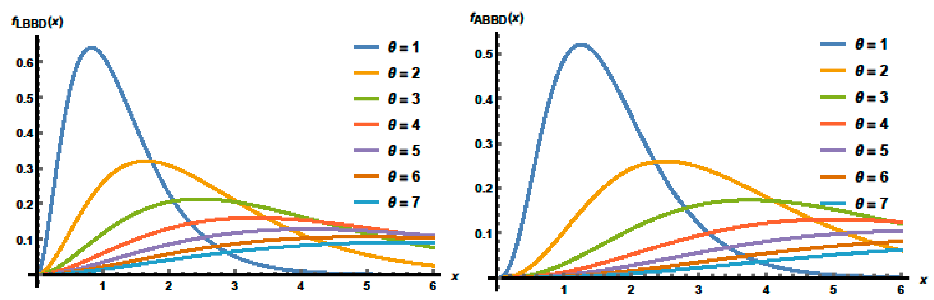
in Equation (5), we obtain the pdfs of the suggested length-biased Bilal distribution (LBBD) and area-biased Bilal distribution (ABBD), respectively:
For various distribution parameter values, the pdf plots of the LBBD and ABBD are shown in
Figure 2. The pdfs of the recommended distributions are skewed to the right and become more flat as the values of
increase. Furthermore, depending on the parameter values, the pdfs of the ABBD and LBBD can display a variety of behaviors.
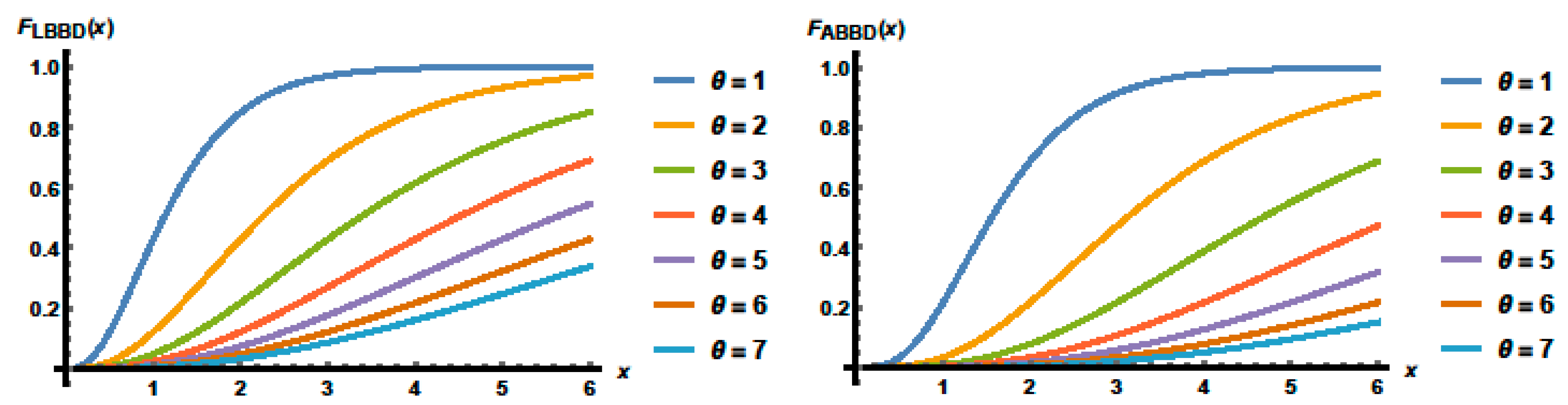
The CDFs of the LBBD and ABBD, respectively, are expressed using the following:
Some of the CDFs plots of the LBBD and ABBD when
are presented in
Figure 3.
3.1. Moments and Related Measure
The moments and related measures, coefficients of variation (Cv), skewness (Sk), and kurtosis (Ku), the incomplete moments and moment of the residual lifetime, moment generating function, reliability functions of the proposed distributions are all described in this section in closed expressions. Also, the parameters estimation, Fisher’s information and entropies, as well as the order statistics are presented.
The
rth moments of the LBBD and ABBD by setting
in Equation (7), respectively, are obtained using the following:
for
and
.
An alternative formulation of a real-valued random variable’s probability distribution is the moment-generating function (mgf). The mgf of the LBBD and ABBD, respectively, are expressed using the following:
The Lorenz ([
19]) and Benforroni [
20] curves are used to measure inequality using the incomplete moments of a probability distribution. The
rth incomplete moments of the LBBD and ABBD from Theorem (2) by setting
, respectively, are defined as follows:
and
The residual life is the time after a component lives up to time
until the time of failure, which is determined by the conditional random variable
. Hence, the
rth moment of the residual lifetime (MRL) of the LBBD and ABBD, respectively, are distinct:
The harmonic means of the LBBD and ABBD are defined as follows:
The
rth quartiles of the LBBD and ABBD, respectively, are the solutions for
in the following equations:
and
where
and
are respectively called the first, second and third quartiles.
The coefficient of skewness is used to determine the skewness of the distribution and is expressed as . For the LBBD and ABBD, correspondingly, the coefficients of skewness are expressed as and
The top of the distribution’s flatness is measured by the coefficient of kurtosis, which can be defined as The LBBD and ABBD has the coefficient of kurtosis and , respectively. The Cv is defined as و and for the LBBD and ABBD, they are expressed as and , respectively.
Table 1 presents the values of the mean and standard deviation (SD) of the LBBD and ABBD for different selections of
. According to
Table 1, as the value of
rises, the mean and standard deviation values of the LBBD and ABBD rise as well.
3.2. Reliability Functions
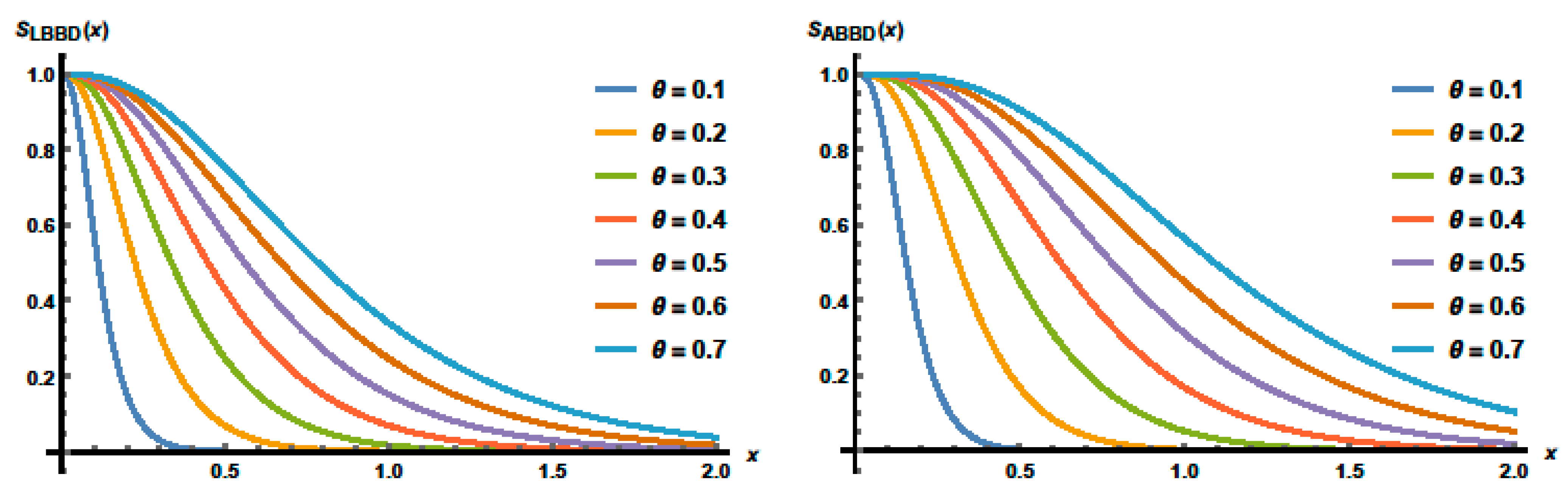
The survival function is frequently used to predict the probability that an event will not occur after a specific amount of time or threshold in domains like survival analysis and reliability engineering, among others. The survival function is defined as
, and for the LBBD and ABBD, respectively, it is characterized as
and
Figure 4 shows the survival functions plots of the LBBD and ABBD for
The plots reveal that the survival functions curves decreases and are skewed to the right. The distances between each two curves depend on the parameters’ values.
In survival analysis and reliability engineering, the hazard function is a basic idea. It is utilized to simulate the instantaneous probability of an event (such as death, failure, or the occurrence of a specific event) occurring at a given time, given that it has not yet happened at that time. It is the ratio between the pdf and survival function of a random variable
X, . For the LBBD and ABBD, the hazard functions, respectively, are expressed using
and
Figure 5 presents the hazard functions of the LBBD and ABBD for some parameter choices, and it is clear that the hazard functions curves are increasing with different ranges depending on the parameter value.
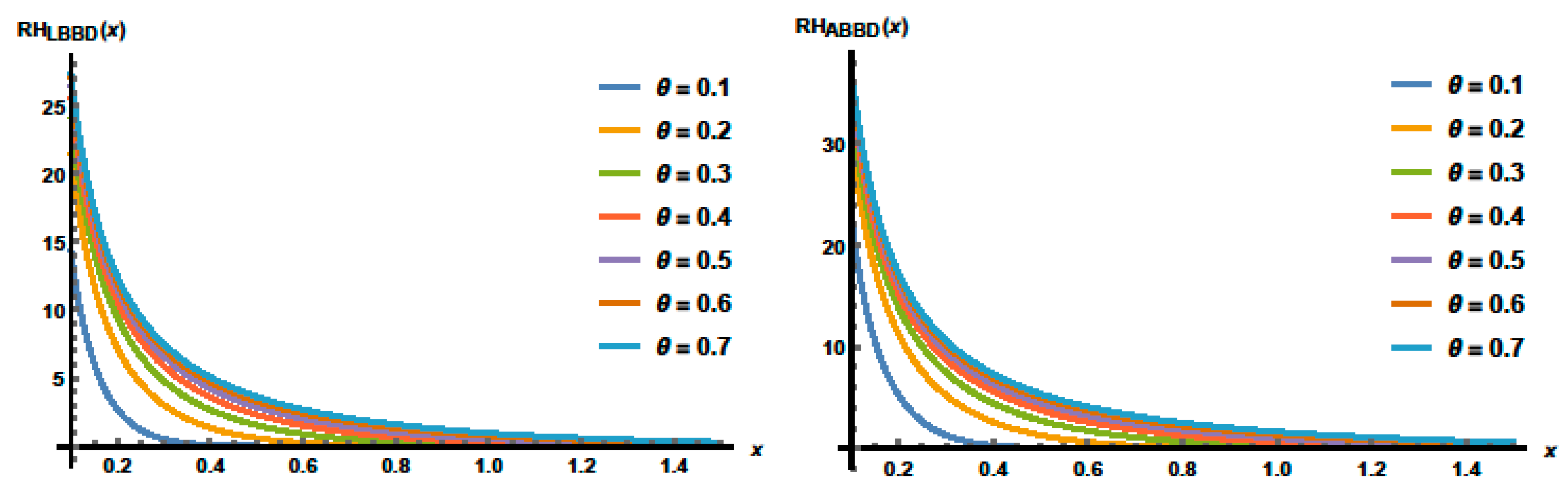
The reversed hazard rate (RH) function is distinct as the ratio between the life probability density to its distribution function as
. The RH functions for the LBBD and ABBD, respectively, are defined as
and
Figure 6 displays some plots of the reversed hazard functions of the LBBD and ABBD for selected values of the parameters as
, where the reversed hazard functions are decreasing for these parameter values.
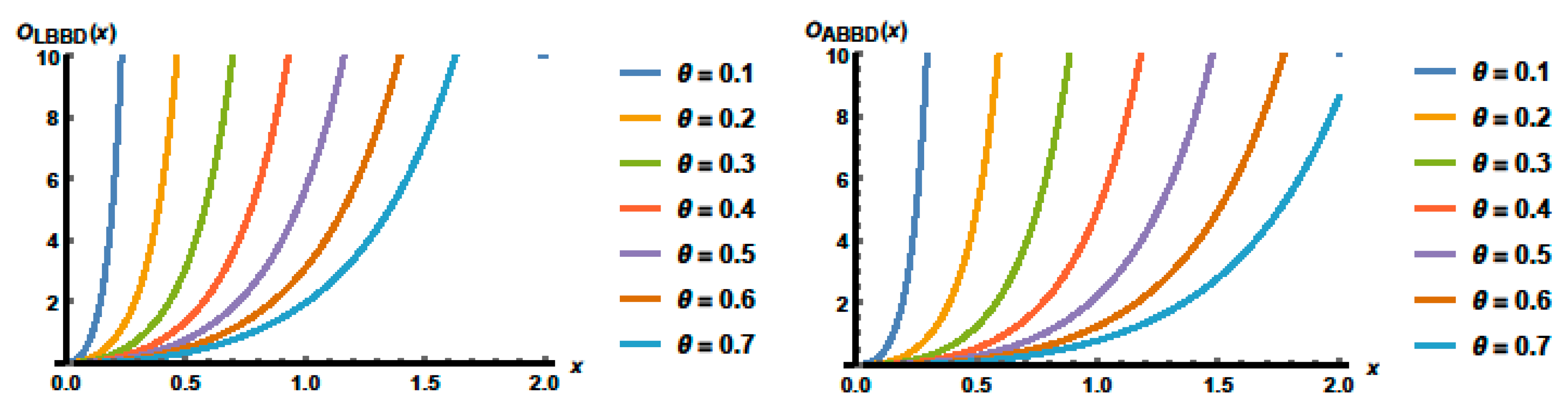
The odds function is obtained as the ratio between
and
as
The LBBD and ABBD have the odds functions, respectively, defined by the following:
Some plots of the odds functions of the LBBD and ABBD for
are presented in
Figure 7, which indicate that the curves are increasing for all parameter values.
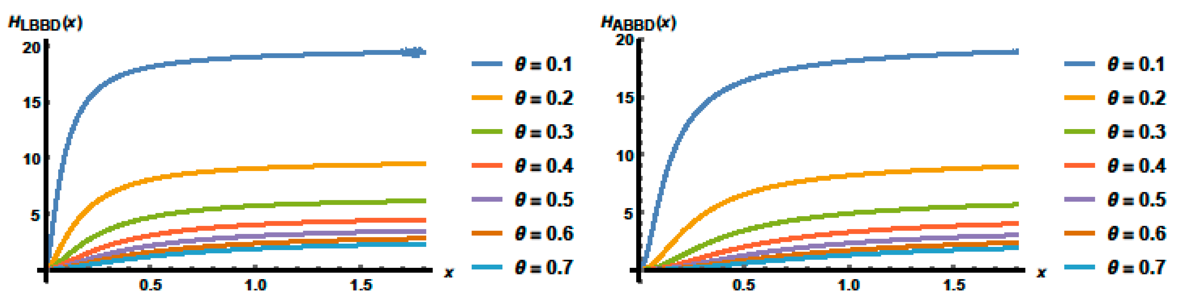
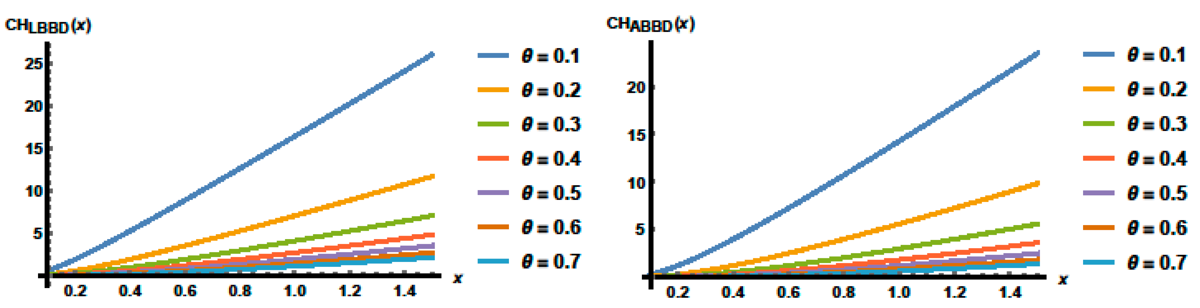
The cumulative hazard (
CH) function of a random variable
X from a univariate continuous distribution is defined as
. The CH for the LBBD and ABBD, respectively, are expressed as
and
Figure 8 shows some plots of the LBBD and ABBD cumulative hazard functions at various values of
It is obvious that the odds function of both distributions is increasing and its values are larger for small values of
.
3.3. Parameters Estimation
The method of moments (MOMs) and maximum likelihood technique are used in this section to estimate the LBBD and ABBD parameters. Let be a random sample of size n selected from a pdf and CDF . The method of moments estimators of the distributions parameter are and , where is the sample mean.
To find the maximum likelihood estimators of the distribution parameter, let
be the sample observations of
from the LBBD and ABBD. The log-likelihood functions are, respectively, obtained using the following:
The partial derivatives of these equations with respect to the parameter
are obtained using the following:
The exact solution of these nonlinear equations is not easy, so one may maximize them by using some optimization approaches as the Newton–Raphson method.
Table 2 provides some values of the MLE
and
, and the corresponding standard errors (SE) for various distributions parameter with sample sizes
n = 40, 80, 120, 160, 200, 240, and 500.
Table 2 demonstrates that the standard errors values for both MLE estimators
and
, which shows that distributions parameters are decreasing for larger sample sizes for fixed parameter values.
3.4. Fisher’s Information and Entropies
This subsection introduces the Fisher’s information (FI) as well as the Rényi entropy of the LBBD and ABBD.
Theorem 5. The Fisher’s information of ABBD and LBBD, respectively, are as follows: Proof. Take the log of the ABBD pdf as
The first and second derivatives of
with respect to
respectively are as follows:
Some values of the Fisher’s information for both of LBBD and ABBD are presented in
Table 3 for selected values of the parameter
.
Table 3 reveals that the values decrease as the distribution’s parameter values rise, and they eventually approach zero for high parameter values.
According to information theory, a random variable’s entropy measures the average amount of uncertainty, information, or surprise that could result from its potential outcomes. From Equation (10), the Rényi entropies of the
LBBD and
ABBD, respectively, are obtained using the following:
Table 4 presents the values of the suggested Rényi entropies of the distributions. It is evident that when the values of
for
increase, the Rényi entropies values decrease. Also, for fixed
, the Rényi entropies values of
are less than their counterparts when
.
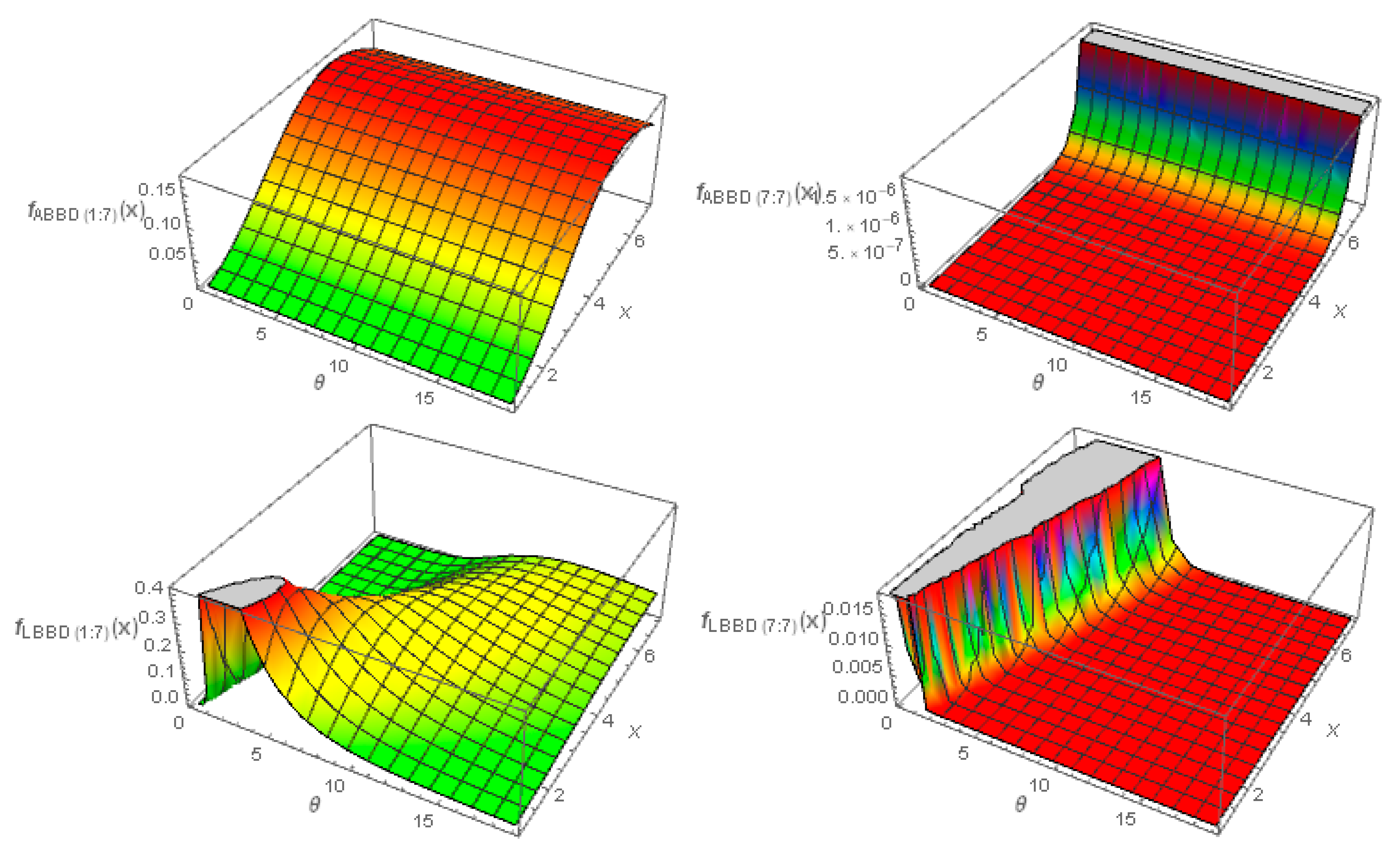
3.5. Order Statistics
In statistical theory, order statistics are essential, especially in the idea of extreme value. Consider a random sample
of size
m selected from
with
Let
be the corresponding order statistics of the sample. The
jth order statistics pdf is defined as follows:
For simplicity, we use
. Now, Equation (15) will be
Therefore, the pdf for the LBBD and ABBD
jth order statistics, respectively, are obtained using
and
For
in Equations (16) and (17), for both LBBD and ABBD, respectively, we can obtain the pdfs of the minimum (min) and maximum (max) order statistics.
Figure 9 shows three-dimensional plots of the pdf of the min and max order statistics of the ABBD and LBBD when
.
4. Applications to Real Data
In this section, we demonstrate the applicability of the proposed ABBD and LBBD distributions using two real data sets.
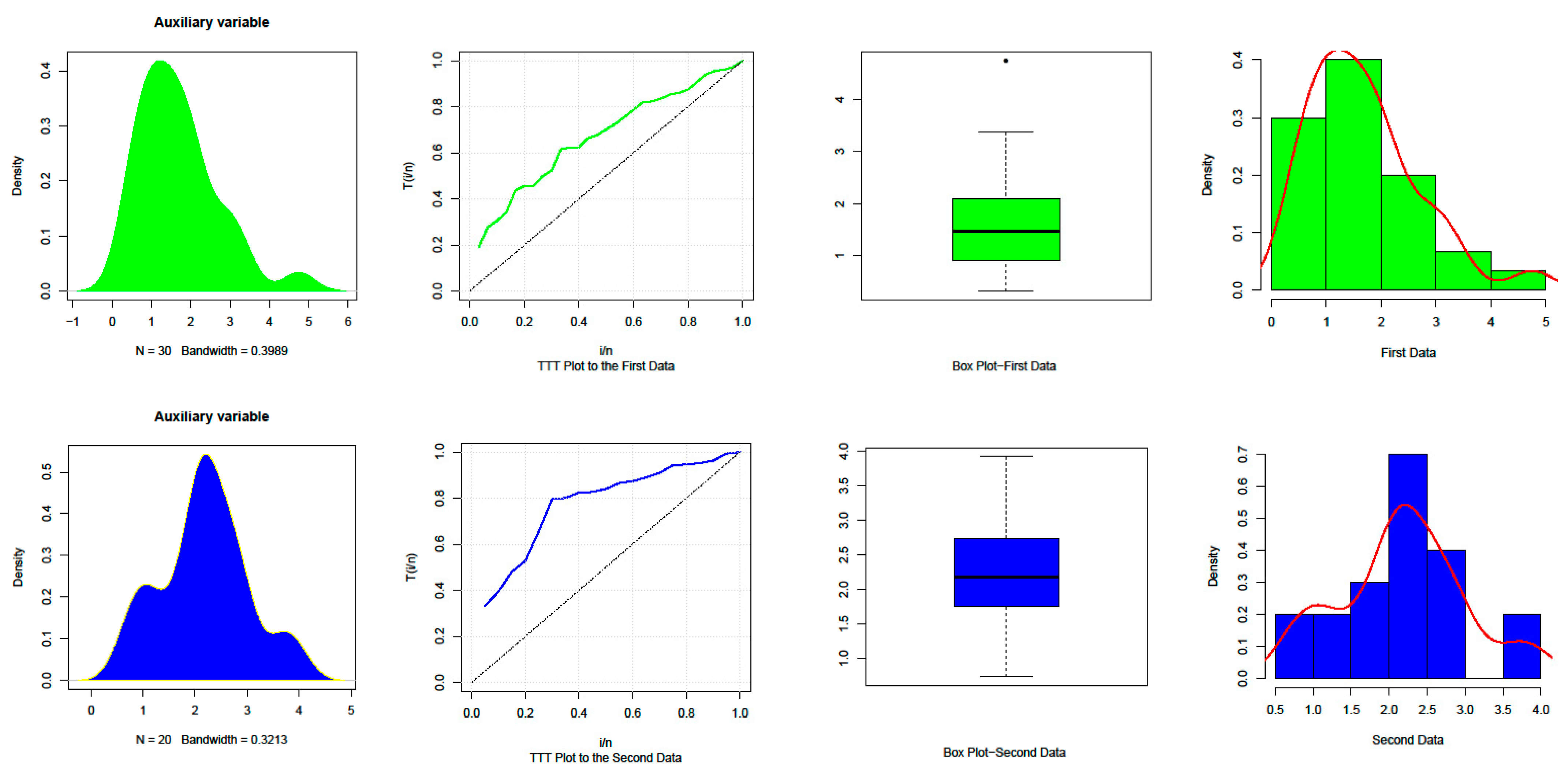
The first data consists of thirty consecutive measurements of March precipitation (in inches) throughout a 30-year period in Minneapolis. The data set values are 0.32, 0.47, 0.52, 0.59, 0.77, 0.81, 0.81, 0.9, 0.96, 1.18, 1.20, 1.20, 1.31, 1.35, 1.43, 1.51, 1.62, 1.74, 1.87, 1.89, 1.95, 2.05, 2.10, 2.20, 2.48, 2.81, 3.0, 3.09, 3.37, and 4.75. The same data are considered by [
21,
22].
The second one consists the survival times (in months) of 20 acute myeloid leukemia patients discussed by [
23], and the observations are 2.226, 2.113, 3.631, 2.473, 2.720, 2.050, 2.061, 3.915, 0.871, 1.548, 2.746, 1.972, 2.265, 1.200, 2.967, 2.808, 1.079, 2.353, 0.726, and 1.958.
The descriptive statistics for both data sets are presented in
Table 5, and it is clear that both data sets are skewed to the right. The density, histogram, box and total time on test (TTT) plots for both data sets are shown in
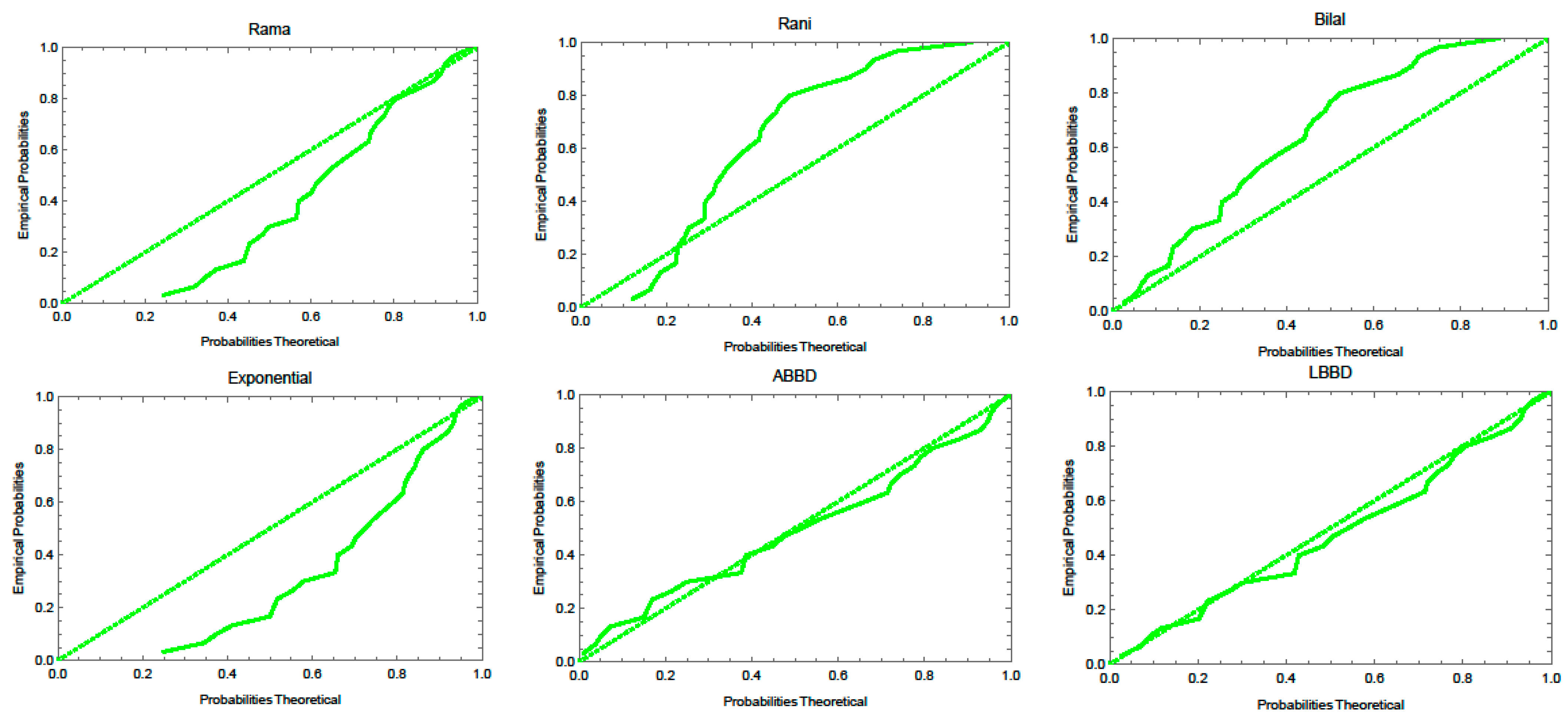
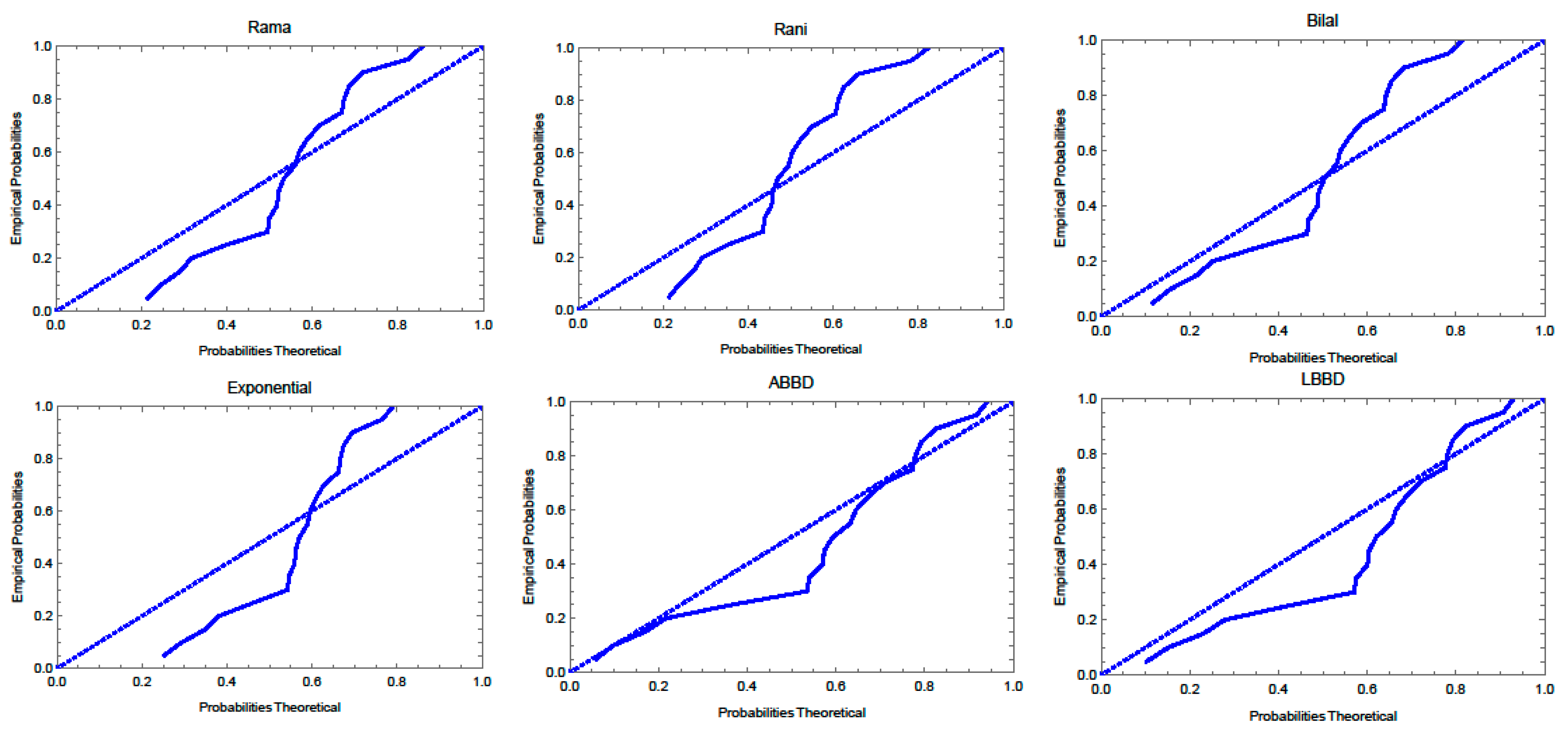
Figure 10. The P-P plots of the fitted distributions for the both data sets are displayed in
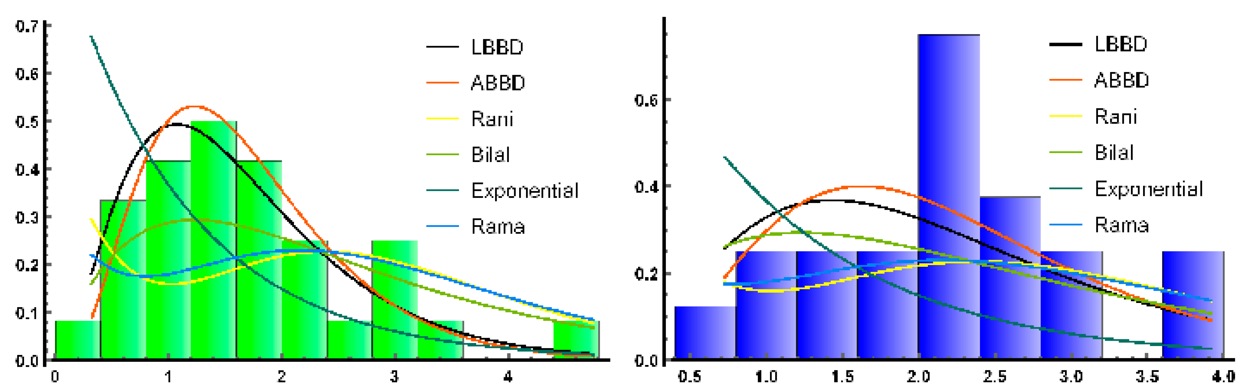
Figure 11. The estimated pdfs of the suggested and competitive distributions are shown in
Figure 12.
Since the proposed distributions in this study have just one parameter, we compared them to certain existing distributions that likewise have just one parameter for a fair comparison.
In order to explain how adaptable LBBD and ABBD are, we are going to evaluate them in contrast to a variety of well-recognized models, including Rani ([
24]), Exponential, Rama ([
25]) and Bilal distributions with pdfs, which are respectively expressed as follows:
- o
- o
- o
- o
We used the maximum likelihood method to estimate these distributions parameters and fit them to the data sets. To compare the results, we used the negative maximized log-likelihood values (
), the Hannan–Quinn information criterion (HQIC), the Bayesian information criterion (BIC), the Akaike information criterion (AIC), and the Consistent Akaike information criterion (CAIC) defined as
,
,
,
, where
n is the sample size and
is the number of parameters. The results are displayed in
Table 6 and the best model is indicated by lower AIC, BIC, CAIC, HQIC values for goodness of statistics. For the first data set, the LBBD fits the data better than other distributions and similarly, the ABBD fits the second data set due to the lowest values of these measures. Therefore, both suggested models are considered as best fitted models as compared to the competitors considered in this study. These results are supported by
Figure 10,
Figure 11 and
Figure 12 where it is seen that the proposed models fit both data sets well.


