Author Contributions
Conceptualization, J.S.C. and J.R.; methodology, M.A.R. and J.R.; software, J.S.C.; validation, J.R. and M.A.R.; formal analysis, J.S.C., M.A.R. and J.R.; investigation, J.S.C., M.A.R. and J.R.; data curation, J.S.C.; writing—original draft preparation, J.S.C., M.A.R. and J.R.; supervision, M.A.R. and J.R. All authors have read and agreed to the published version of the manuscript.
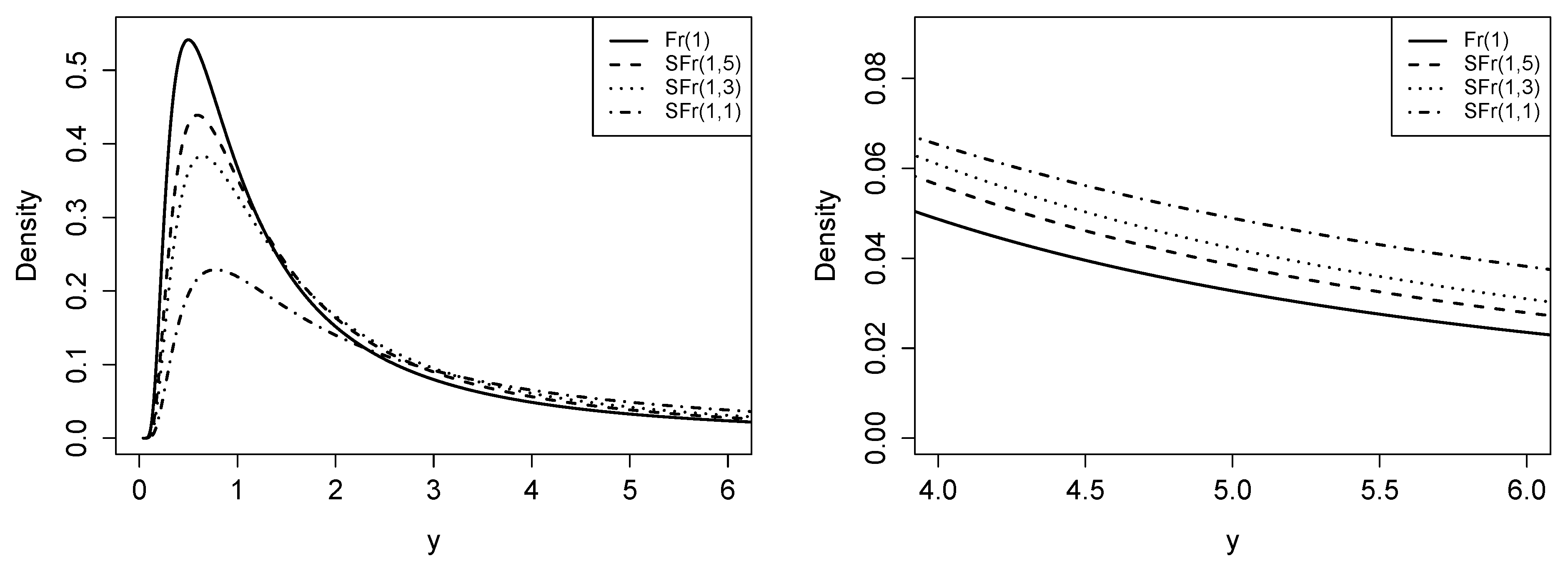
Figure 1.
Graphical comparison of the density function of the Fréchet (Fr) and slash Fréchet (SFr) distributions for fixed alpha () and different values of q.
Figure 1.
Graphical comparison of the density function of the Fréchet (Fr) and slash Fréchet (SFr) distributions for fixed alpha () and different values of q.
Figure 2.
Graphical comparison of the CDF between the Fréchet (Fr) and slash Fréchet (SFr) distribution for the fixed alpha () and different values of q.
Figure 2.
Graphical comparison of the CDF between the Fréchet (Fr) and slash Fréchet (SFr) distribution for the fixed alpha () and different values of q.
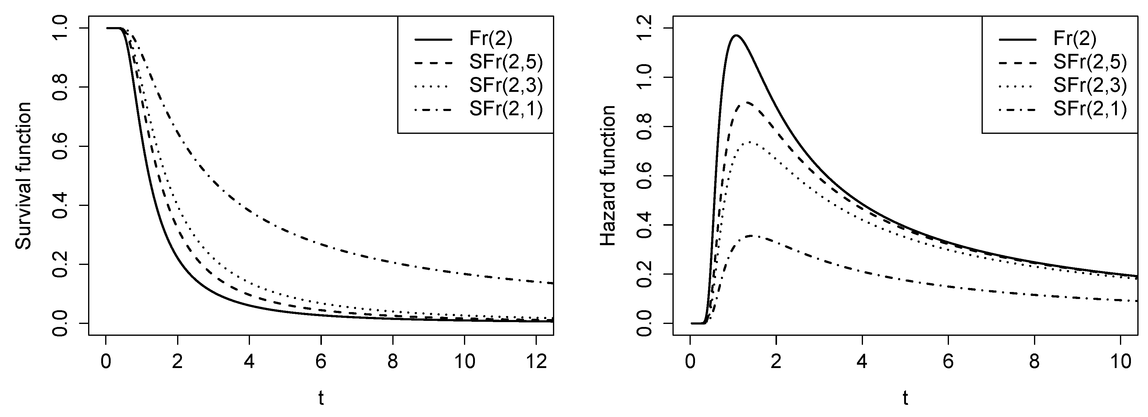
Figure 3.
Graphs of the survival function and hazard function for the SFr distribution with and different values of q.
Figure 3.
Graphs of the survival function and hazard function for the SFr distribution with and different values of q.
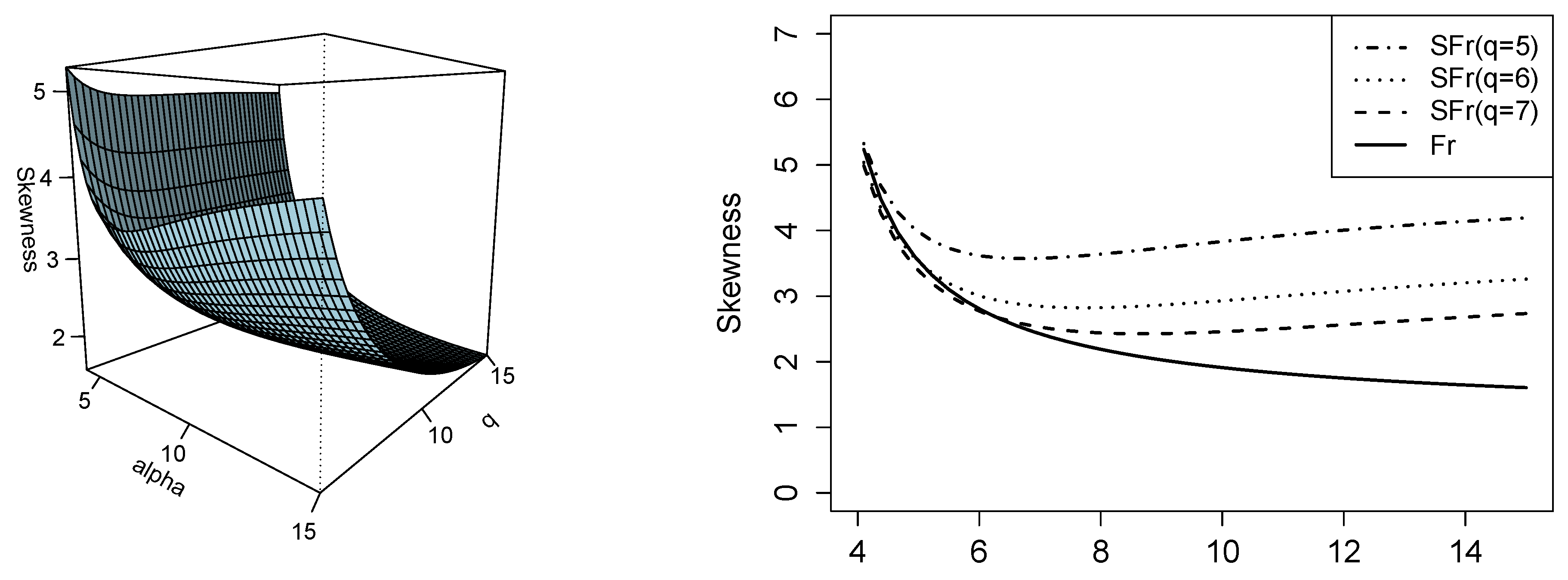
Figure 4.
Skewness coefficient plot of the SFr model (left side). Comparison of the skewness coefficient between SFr and Fr for different values of q (right side).
Figure 4.
Skewness coefficient plot of the SFr model (left side). Comparison of the skewness coefficient between SFr and Fr for different values of q (right side).
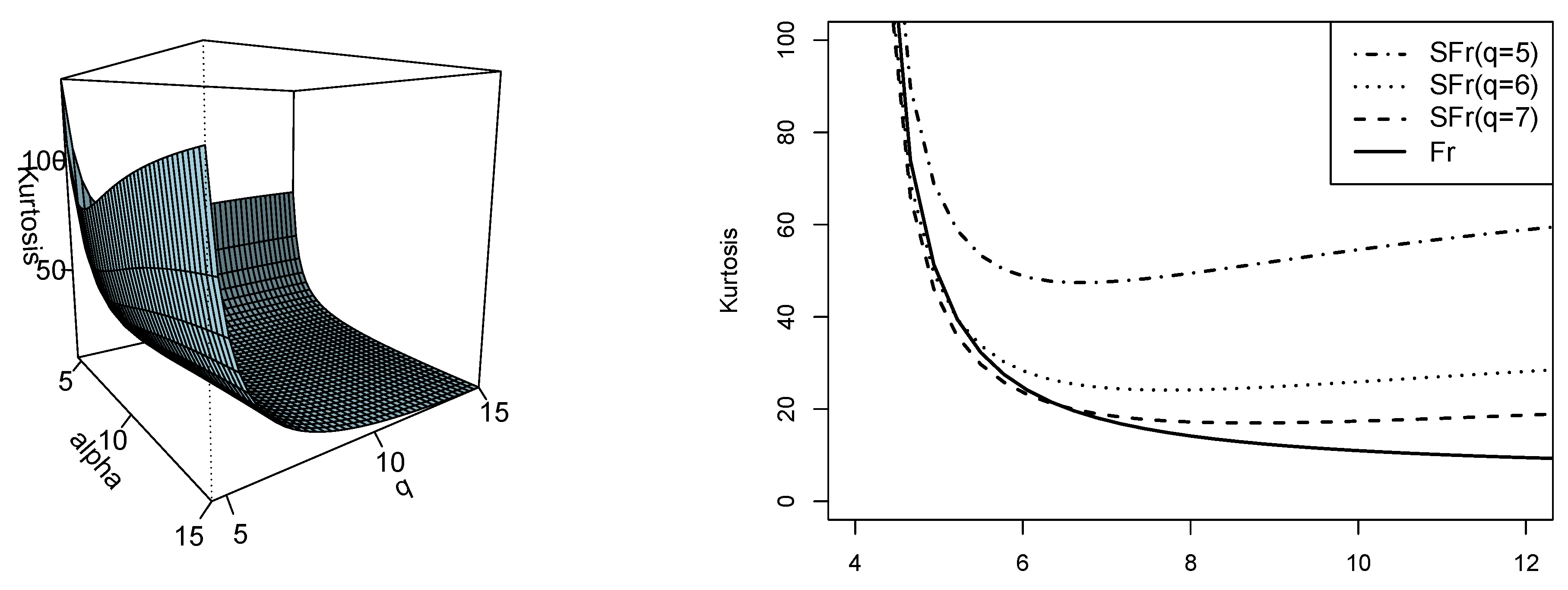
Figure 5.
Plot of the kurtosis coefficient for the SFr model (left side). Comparison of the kurtosis coefficient between the SFr and Fr models for different values of q (right side).
Figure 5.
Plot of the kurtosis coefficient for the SFr model (left side). Comparison of the kurtosis coefficient between the SFr and Fr models for different values of q (right side).
Figure 6.
Profile of the log-likelihood of the SFr distribution.
Figure 6.
Profile of the log-likelihood of the SFr distribution.
Figure 7.
Box plot for the dataset of patients undergoing lung cancer.
Figure 7.
Box plot for the dataset of patients undergoing lung cancer.
Figure 8.
Density adjusted for the dataset of patients undergoing lung cancer in the Fr and SFr distributions.
Figure 8.
Density adjusted for the dataset of patients undergoing lung cancer in the Fr and SFr distributions.
Figure 9.
QQ plots for the dataset of patients undergoing lung cancer: (a) Fr Model; (b) SFr model.
Figure 9.
QQ plots for the dataset of patients undergoing lung cancer: (a) Fr Model; (b) SFr model.
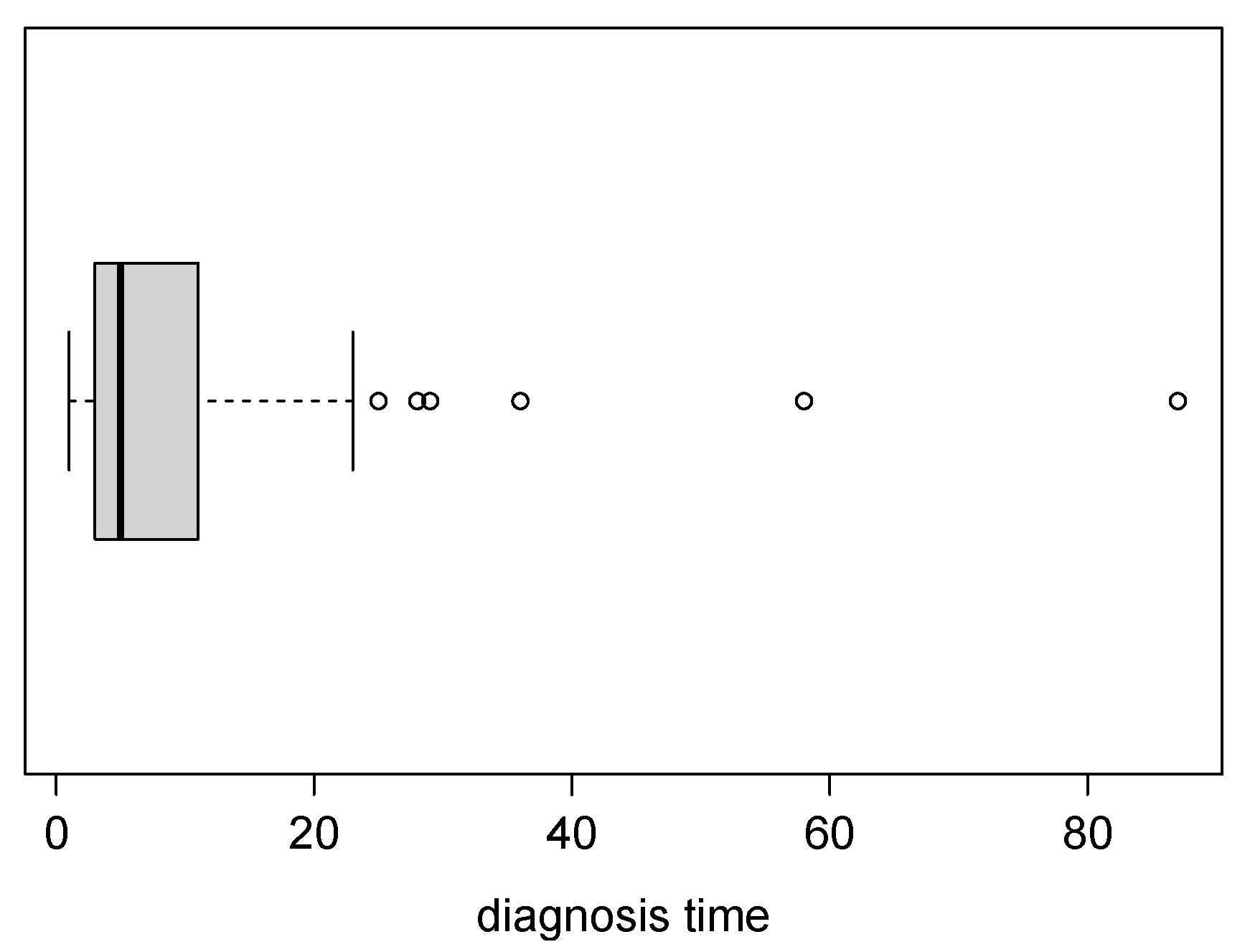
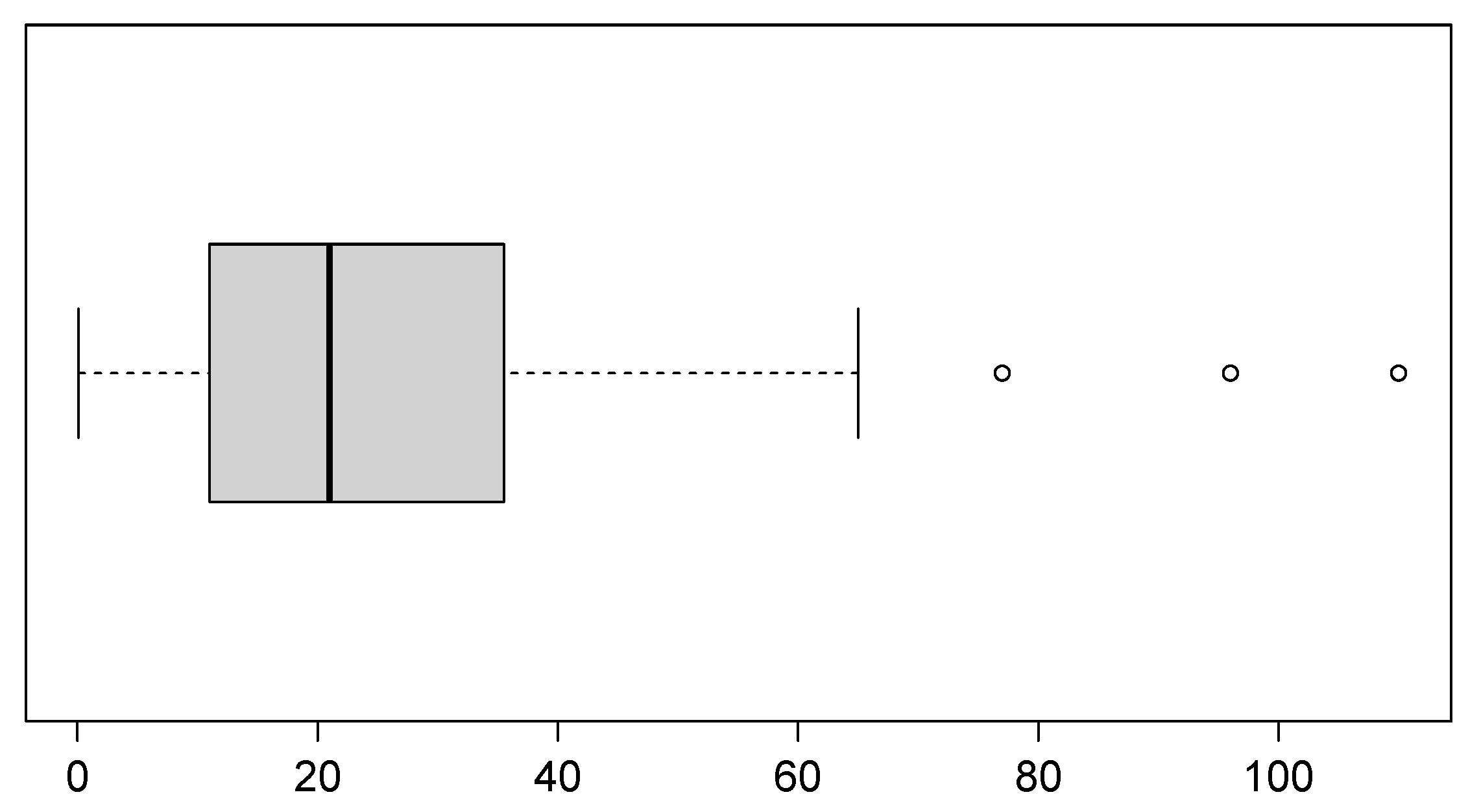
Figure 10.
Box plot of the dataset of patients undergoing peritoneal dialysis.
Figure 10.
Box plot of the dataset of patients undergoing peritoneal dialysis.
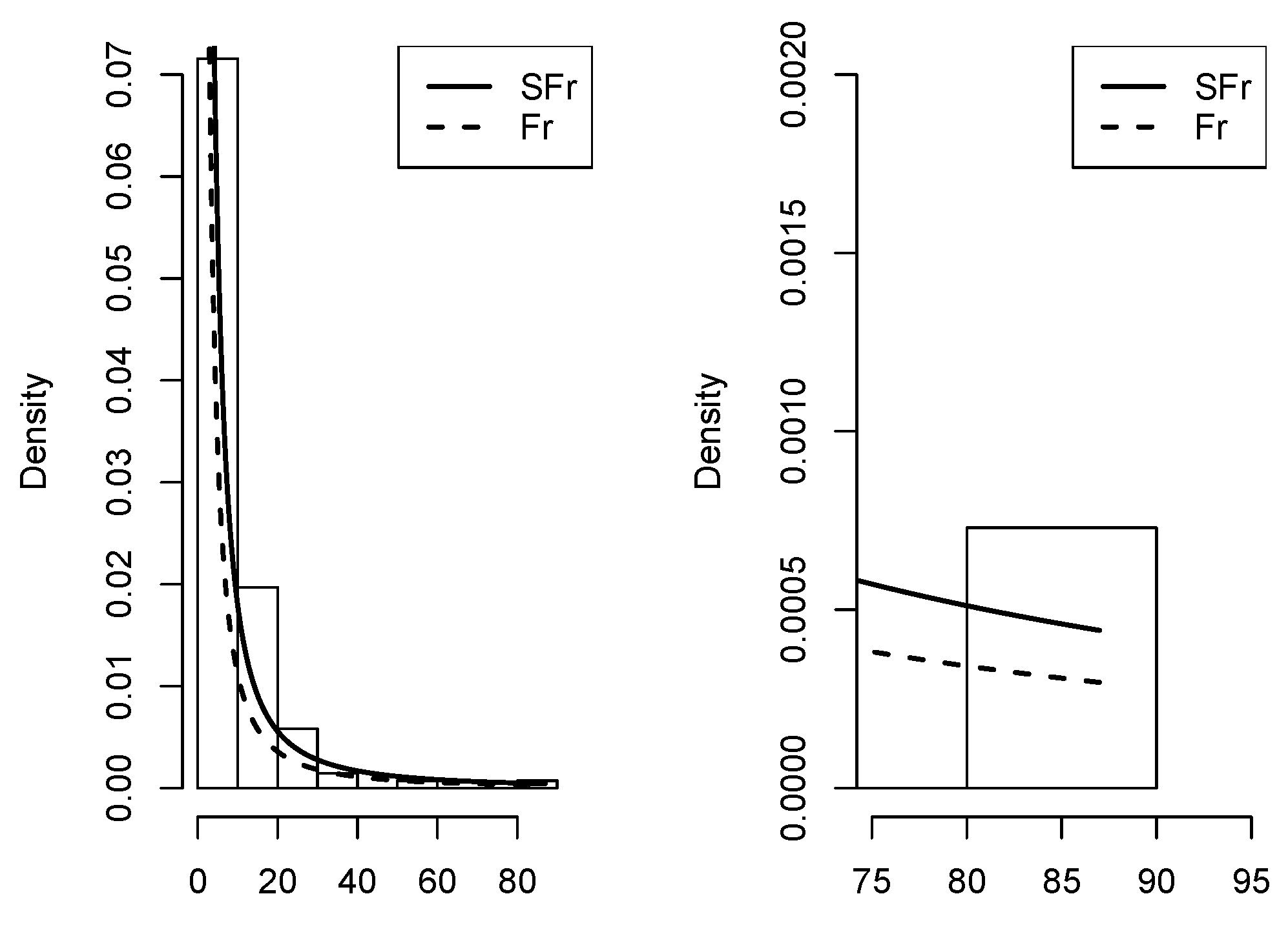
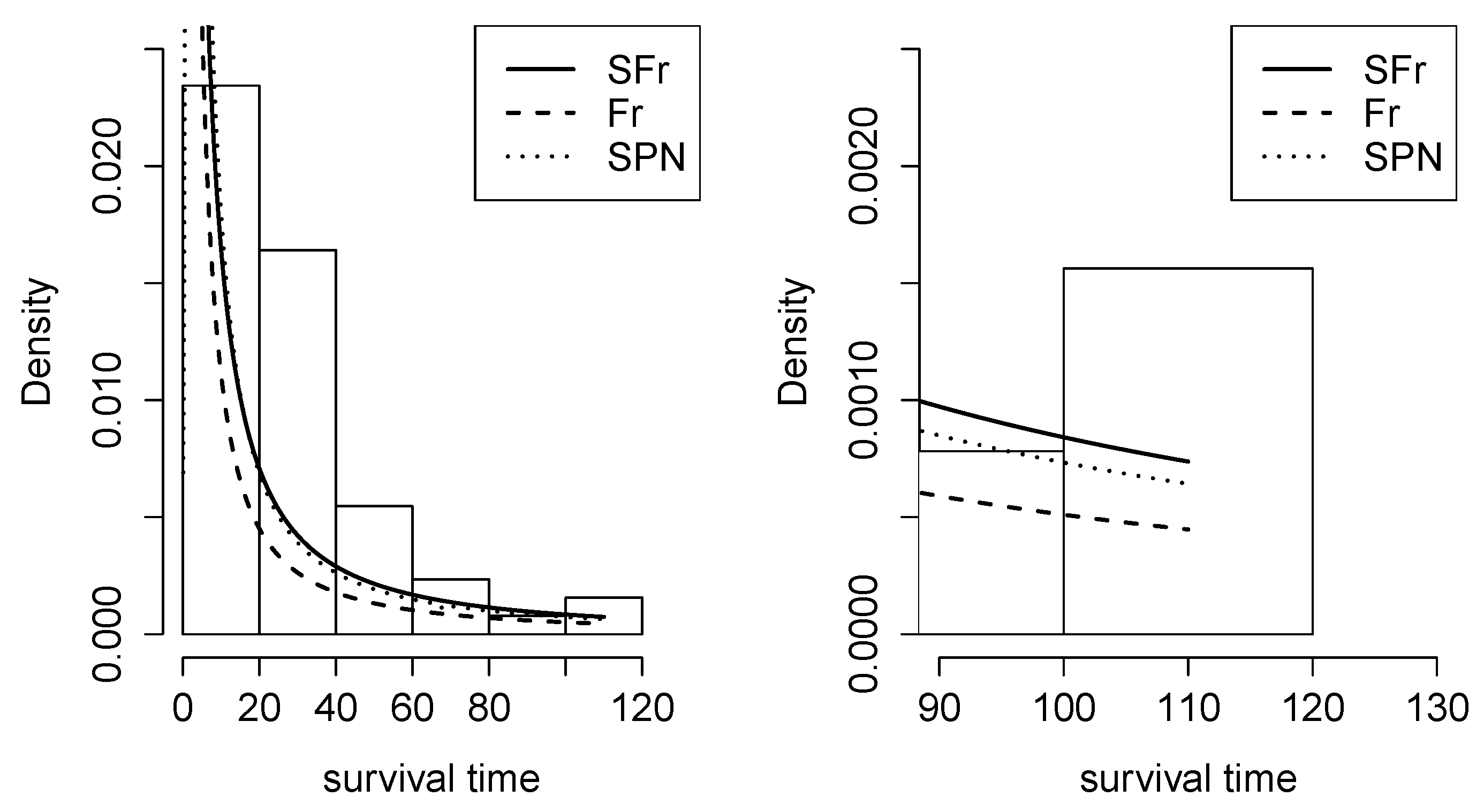
Figure 11.
Density adjusted to the dataset of patients undergoing peritoneal dialysis in the Fr, SPN, and SFr distributions.
Figure 11.
Density adjusted to the dataset of patients undergoing peritoneal dialysis in the Fr, SPN, and SFr distributions.
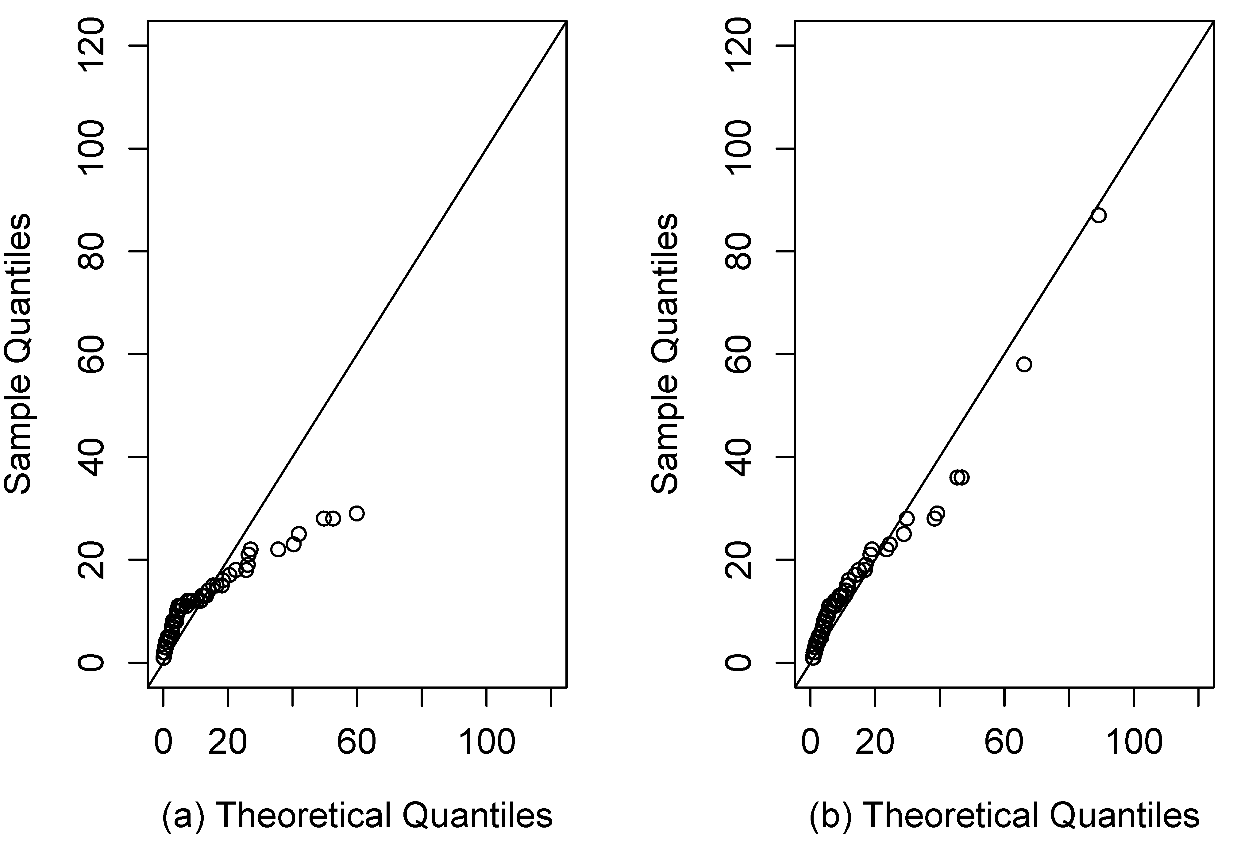
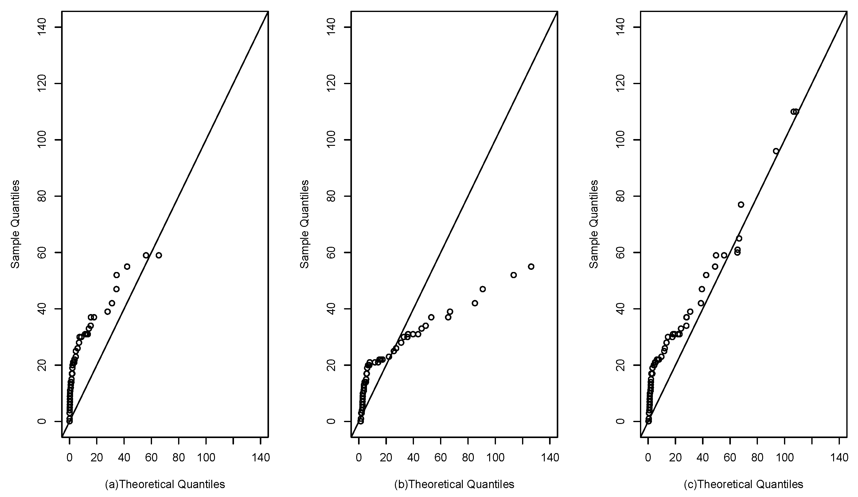
Figure 12.
QQ plots for the dataset of patients undergoing peritoneal dialysis: (a) Fr model; (b) SPN model; (c) SFr model.
Figure 12.
QQ plots for the dataset of patients undergoing peritoneal dialysis: (a) Fr model; (b) SPN model; (c) SFr model.
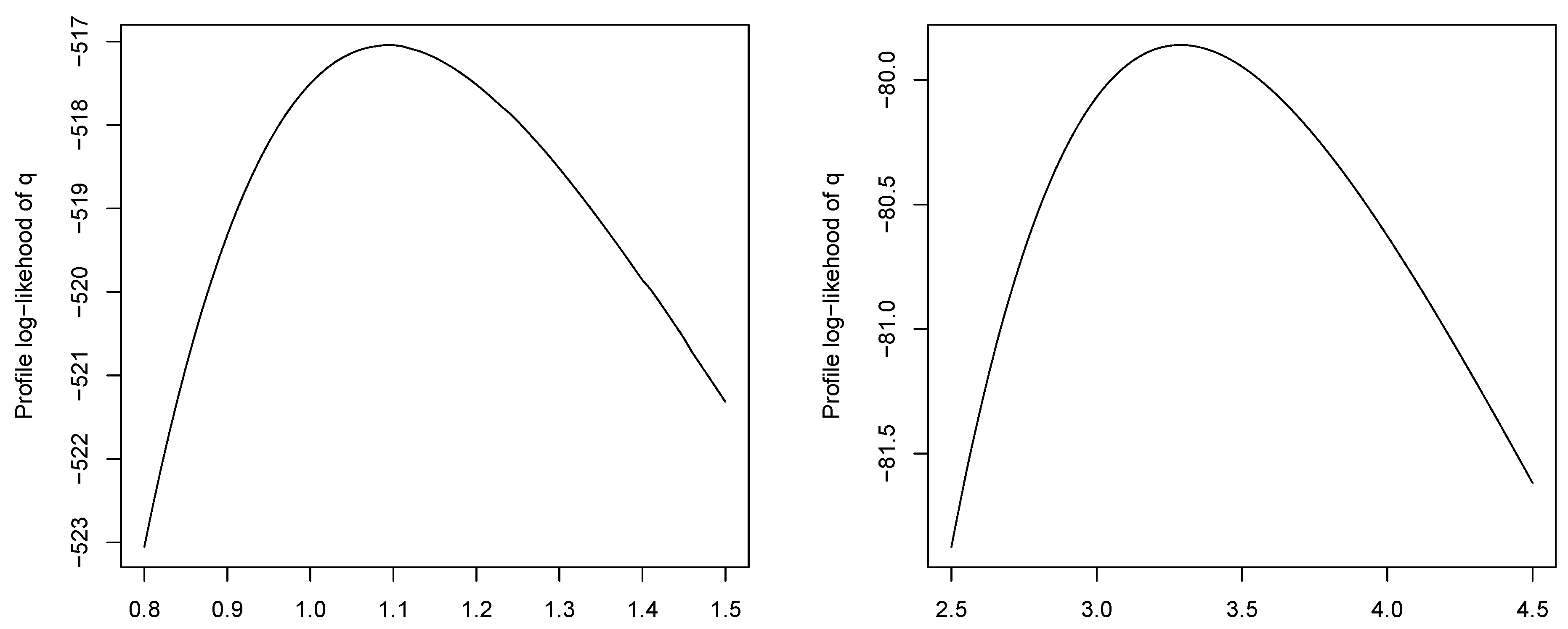
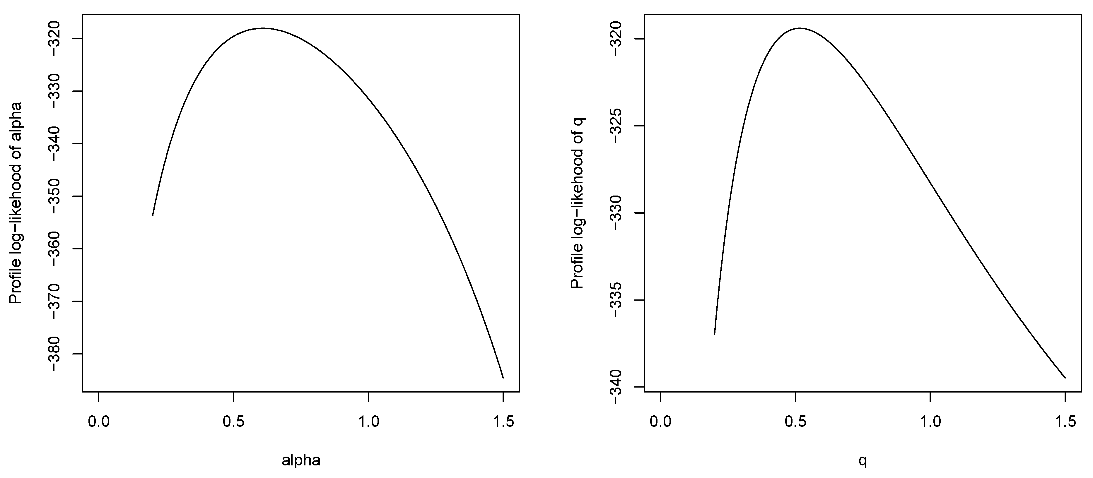
Figure 13.
Profile log-likelihoods of and q for the dataset of patients undergoing peritoneal dialysis.
Figure 13.
Profile log-likelihoods of and q for the dataset of patients undergoing peritoneal dialysis.
Figure 14.
Box plot for the dataset of patients undergoing breast cancer.
Figure 14.
Box plot for the dataset of patients undergoing breast cancer.
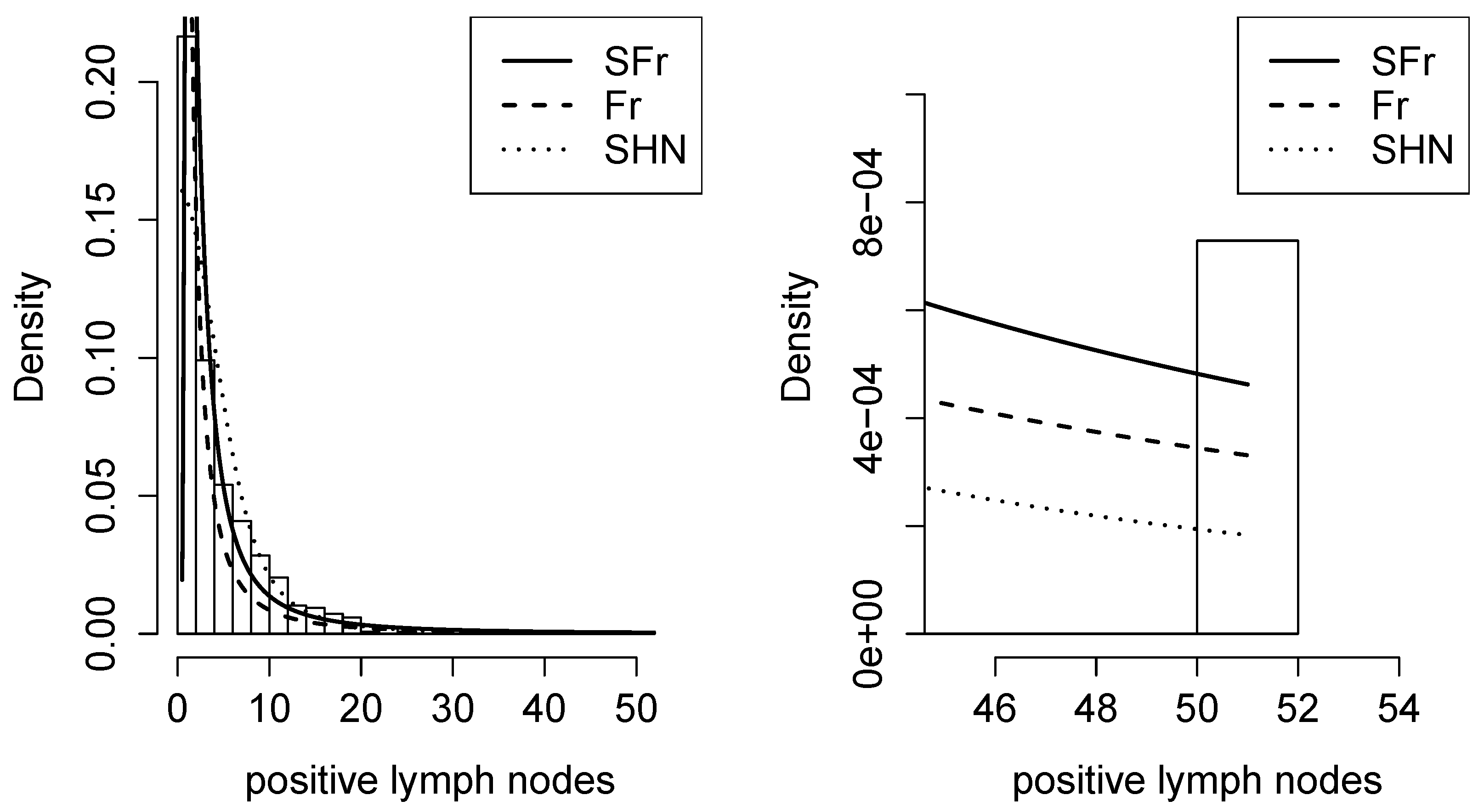
Figure 15.
Density adjusted for the dataset of patients undergoing breast cancer in the Fr, SHN, and SFr distributions.
Figure 15.
Density adjusted for the dataset of patients undergoing breast cancer in the Fr, SHN, and SFr distributions.
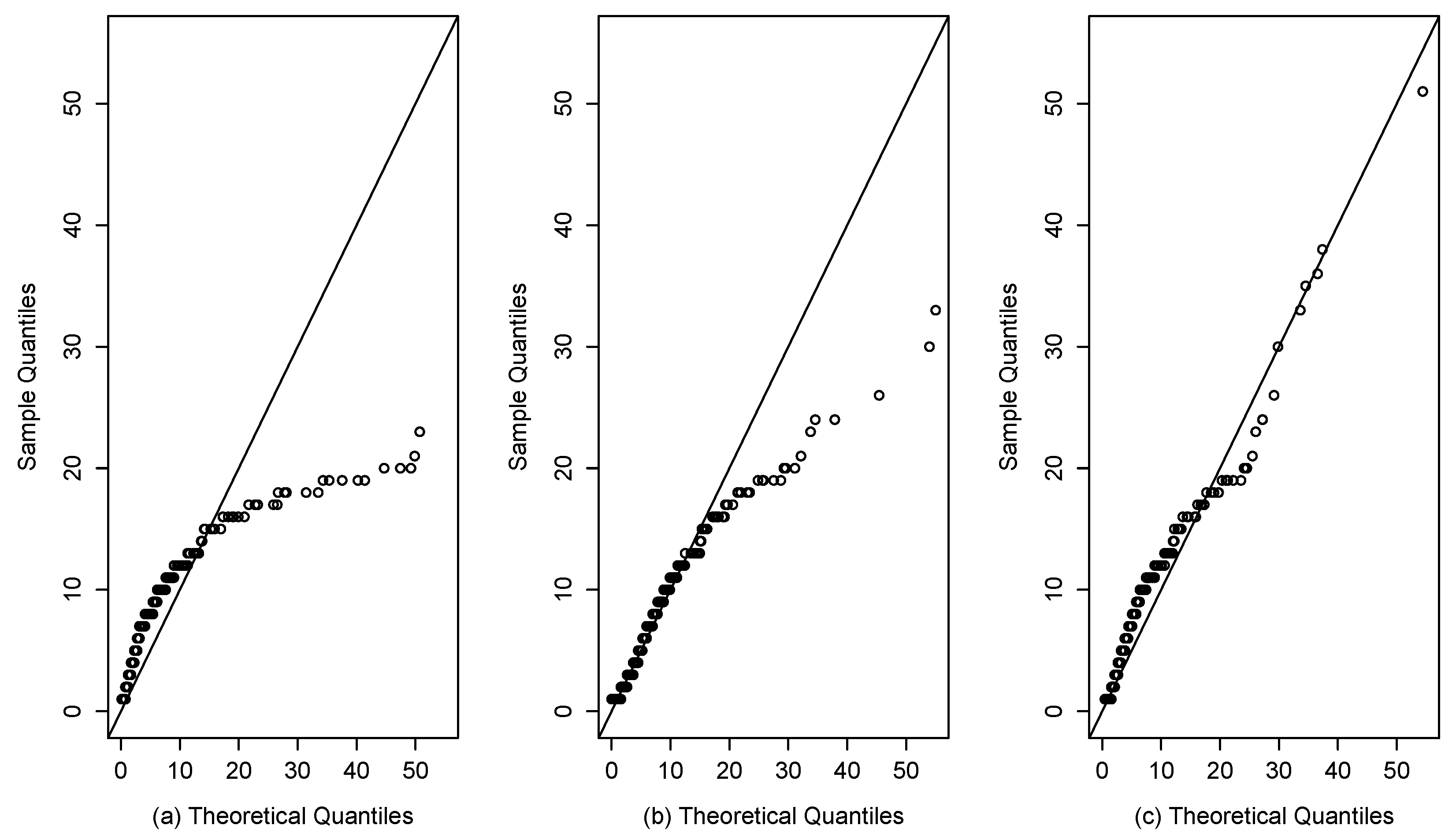
Figure 16.
QQ plots for the dataset of patients undergoing breast cancer: (a) Fr model; (b) SHN model (c) SFr model.
Figure 16.
QQ plots for the dataset of patients undergoing breast cancer: (a) Fr model; (b) SHN model (c) SFr model.
Table 1.
Comparison of values of the survival function between the SFr and Fr distributions for and q = 1, 3, 5, 10.
Table 1.
Comparison of values of the survival function between the SFr and Fr distributions for and q = 1, 3, 5, 10.
| | | | | |
|---|
| Fr (1) | 0.0952 | 0.0869 | 0.0800 | 0.0740 | 0.0689 |
| SFr (1, 10) | 0.1051 | 0.0960 | 0.0884 | 0.0819 | 0.0763 |
| SFr (1, 5) | 0.1171 | 0.1070 | 0.0986 | 0.0914 | 0.0852 |
| SFr (1, 3) | 0.1368 | 0.1253 | 0.1157 | 0.1074 | 0.1002 |
| SFr (1, 1) | 0.2775 | 0.2605 | 0.2457 | 0.2327 | 0.2212 |
Table 2.
Simulation of 2000 samples for the model.
Table 2.
Simulation of 2000 samples for the model.
| n | | q | | | | | | |
|---|
| 50 | 0.5 | 0.5 | 0.5544 | 0.1156 | 97.35 | 0.5329 | 0.1574 | 90.45 |
| 100 | 0.5225 | 0.0676 | 96.05 | 0.5141 | 0.0972 | 92.65 |
| 150 | 0.5148 | 0.0536 | 95.65 | 0.5074 | 0.0775 | 93.20 |
| 200 | 0.5109 | 0.0455 | 95.65 | 0.5061 | 0.0664 | 93.75 |
| 250 | 0.5068 | 0.0401 | 95.15 | 0.5052 | 0.0593 | 94.30 |
| 300 | 0.5068 | 0.0367 | 95.20 | 0.5035 | 0.0539 | 95.05 |
| 50 | 0.7 | 0.4 | 0.8964 | 0.4138 | 97.60 | 0.4106 | 0.0833 | 93.20 |
| 100 | 0.7438 | 0.1289 | 96.95 | 0.4059 | 0.0570 | 94.80 |
| 150 | 0.7307 | 0.1006 | 95.75 | 0.4032 | 0.0457 | 94.65 |
| 200 | 0.7205 | 0.0845 | 95.25 | 0.4025 | 0.0394 | 94.80 |
| 250 | 0.7160 | 0.0747 | 96.25 | 0.4022 | 0.0351 | 95.10 |
| 300 | 0.7151 | 0.0681 | 95.45 | 0.4007 | 0.0318 | 93.95 |
| 50 | 1 | 1 | 1.1888 | 0.3298 | 96.90 | 1.0482 | 0.2915 | 90.1 |
| 100 | 1.0416 | 0.1342 | 95.75 | 1.0178 | 0.1910 | 94.1 |
| 150 | 1.0276 | 0.1066 | 95.40 | 1.0159 | 0.1550 | 93.3 |
| 200 | 1.0200 | 0.0909 | 95.00 | 1.0088 | 0.1322 | 92.8 |
| 250 | 1.0147 | 0.0805 | 95.35 | 1.0096 | 0.1187 | 94.4 |
| 300 | 1.0122 | 0.0731 | 95.30 | 1.0073 | 0.1078 | 94.4 |
| 50 | 3 | 2 | 3.5152 | 2.6864 | 97.25 | 2.0399 | 0.4426 | 93.25 |
| 100 | 3.1753 | 0.5104 | 96.30 | 2.0275 | 0.3054 | 94.80 |
| 150 | 3.1360 | 0.4020 | 96.20 | 2.0132 | 0.2444 | 93.75 |
| 200 | 3.0860 | 0.3375 | 95.45 | 2.0124 | 0.2113 | 94.85 |
| 250 | 3.0645 | 0.2973 | 96.05 | 2.0127 | 0.1885 | 94.60 |
| 300 | 3.0498 | 0.2694 | 96.25 | 2.0065 | 0.1712 | 95.50 |
| 50 | 5 | 3 | 6.0466 | 2.2275 | 96.55 | 3.0638 | 0.6347 | 93.05 |
| 100 | 5.3670 | 0.9570 | 96.45 | 3.0306 | 0.4333 | 94.10 |
| 150 | 5.1994 | 0.6965 | 95.70 | 3.0305 | 0.3513 | 94.80 |
| 200 | 5.1491 | 0.5910 | 96.35 | 3.0132 | 0.3003 | 95.25 |
| 250 | 5.1065 | 0.5197 | 95.25 | 3.0230 | 0.2699 | 94.65 |
| 300 | 5.0991 | 0.4726 | 95.45 | 3.0158 | 0.2451 | 95.30 |
| 50 | 2.3 | 2 | 2.5672 | 0.5551 | 96.65 | 2.0735 | 0.5295 | 91.60 |
| 100 | 2.3919 | 0.3308 | 96.00 | 2.0451 | 0.3593 | 93.55 |
| 150 | 2.3612 | 0.2624 | 95.85 | 2.0196 | 0.2835 | 94.75 |
| 200 | 2.3540 | 0.2253 | 95.65 | 2.0190 | 0.2449 | 95.20 |
| 250 | 2.3387 | 0.1994 | 95.05 | 2.0171 | 0.2186 | 95.35 |
| 300 | 2.3378 | 0.1816 | 95.25 | 2.0128 | 0.1983 | 95.15 |
| 50 | 4.5 | 5 | 4.8658 | 0.8912 | 96.75 | 5.2956 | 1.6178 | 91.10 |
| 100 | 4.6657 | 0.5677 | 96.05 | 5.1339 | 1.0337 | 92.45 |
| 150 | 4.6148 | 0.4520 | 95.50 | 5.1018 | 0.8302 | 92.35 |
| 200 | 4.5990 | 0.3896 | 94.40 | 5.0426 | 0.7024 | 93.25 |
| 250 | 4.5751 | 0.3441 | 95.25 | 5.0352 | 0.6242 | 93.85 |
| 300 | 4.5670 | 0.3126 | 94.20 | 5.0394 | 0.5719 | 93.45 |
Table 3.
Descriptive statistics for the dataset of patients undergoing lung cancer.
Table 3.
Descriptive statistics for the dataset of patients undergoing lung cancer.
| n | | S | | |
|---|
| 137 | 8.7737 | 10.6121 | 4.1055 | 26.3882 |
Table 4.
Estimates, SE in parenthesis, log-likelihood, AIC, BIC, CAIC, and HQIC values for the dataset of patients undergoing lung cancer.
Table 4.
Estimates, SE in parenthesis, log-likelihood, AIC, BIC, CAIC, and HQIC values for the dataset of patients undergoing lung cancer.
| Parameters | Fr | SFr |
|---|
| 0.7452 (0.0540) | 2.0245 (0.3805) |
| q | - | 0.7382 (0.0812) |
| log-likelihood | −504.6068 | −444.1976 |
| AIC | 1011.214 | 892.3952 |
| BIC | 1014.134 | 898.2351 |
| CAIC | 1015.134 | 900.2351 |
| HQIC | 1012.400 | 894.7684 |
Table 5.
Descriptive statistics for the dataset of patients undergoing peritoneal dialysis.
Table 5.
Descriptive statistics for the dataset of patients undergoing peritoneal dialysis.
| n | | S | | |
|---|
| 64 | 27.9547 | 24.9442 | 1.5772 | 5.4244 |
Table 6.
Estimates, SE in parenthesis, log-likelihood, AIC, BIC, CAIC, and HQIC values for the dataset of patients undergoing peritoneal dialysis.
Table 6.
Estimates, SE in parenthesis, log-likelihood, AIC, BIC, CAIC, and HQIC values for the dataset of patients undergoing peritoneal dialysis.
| Parameters | Fr | SPN | SFr |
|---|
| 0.4377 (0.0446) | - | 0.6679 (0.0767) |
| - | 8.6409 (1.9018) | - |
| q | - | 0.3900 (0.0509) | 0.5794 (0.1025) |
| log-likelihood | −336.0071 | −319.3558 | −315.4611 |
| AIC | 674.0141 | 642.7116 | 634.9221 |
| BIC | 676.1730 | 647.0294 | 639.2399 |
| CAIC | 677.1730 | 649.0294 | 641.2399 |
| HQIC | 674.8646 | 644.4126 | 636.6231 |
Table 7.
Descriptive statistics for the dataset of patients undergoing breast cancer.
Table 7.
Descriptive statistics for the dataset of patients undergoing breast cancer.
| n | | S | | |
|---|
| 686 | 5.0102 | 5.4755 | 2.8784 | 16.2079 |
Table 8.
Estimates, SE in parenthesis, log-likelihood, AIC, BIC, CAIC, and HQIC values for the dataset of patients undergoing breast cancer.
Table 8.
Estimates, SE in parenthesis, log-likelihood, AIC, BIC, CAIC, and HQIC values for the dataset of patients undergoing breast cancer.
| Parameters | Fr | SHN | SFr |
|---|
| 1.0452 (0.0348) | - | 2.2209 (0.1934) |
| - | 3.2493 (0.2384) | - |
| q | - | 1.9260 (0.2031) | 1.1304 (0.0631) |
| log-likelihood | −1905.598 | −1790.6070 | −1712.0270 |
| AIC | 3813.196 | 3585.215 | 3428.054 |
| BIC | 3817.727 | 3594.277 | 3437.116 |
| CAIC | 3818.727 | 3596.277 | 3439.116 |
| HQIC | 3814.949 | 3588.721 | 3431.561 |


