
Numerical Analysis of Fractional-Order Parabolic Equation Involving Atangana–Baleanu Derivative

Department of Mathematics, College of Science, University of Bisha, Bisha 61922, Saudi Arabia
Symmetry 2023, 15(1), 237; https://doi.org/10.3390/sym15010237
Submission received: 5 January 2023
/
Revised: 11 January 2023
/
Accepted: 12 January 2023
/
Published: 15 January 2023
(This article belongs to the Special Issue Symmetry in Quantum Calculus)
Abstract
:In this study, the suggested q-homotopy analysis transform method is used to compute a numerical solution of a fractional parabolic equation, and the solution is obtained in a fast convergent series. The leverage and efficacy of the suggested technique are demonstrated by the test examples provided. The results that were acquired are graphically displayed. The series solution in a sizable admissible domain is handled in an extreme way by the current method. It provides us with a simple means of modifying the solution’s convergence zone. The effectiveness and potential of the suggested algorithm are explicitly shown in the results using graphs.
1. Introduction
Fractional calculus is the study of arbitrary order differential and integral equations (FC). Newton invented FC, but it has only recently garnered the interest of a number of specialists. Within the framework of FC, the most intriguing advances in engineering and science applications have been produced over the past three decades. Due to the intrinsic complexity of heterogeneous processes, the non-integer derivative concept has been industrialized. Using fractional differential operators, one can model the behavior of multidimensional media undergoing a diffusion process [1,2,3]. Fractional order differential equations have shown to be a very useful tool, allowing for clearer and more precise solutions to numerous situations. As a result of the rapid rise of mathematical procedures utilizing computer software, a large number of academics began working on extended calculus in order to express their perspectives while analyzing a vast array of complex phenomena [4,5,6]. Consequently, symmetry analysis is a useful method for comprehending partial differential equations, particularly when examining equations generated from accounting-related mathematical concepts. Despite the notion that symmetry is the foundation of nature, “most” observations of the natural world lack symmetry. Creating unexpected events that break symmetry is a creative technique to conceal symmetry. There are two varieties of symmetry: finite and infinitesimal. Both discrete and continuous finite symmetries exist in two distinct forms. Parity and temporal inversion are instances of "discrete" natural symmetries, whereas space represents a continuous change. Mathematicians have always been fascinated by patterns. In the seventeenth century, classification of spatial and planar patterns gained off [7,8,9,10].
Distinguished researchers have provided a variety of ground-breaking recommendations for the several FC definitions that served as the basis. [11,12,13]. FC has also been associated with practical endeavors and is frequently employed in chaos soliton theory [14], optics [15], nanotechnology [16], human diseases [17], and other fields [18,19,20,21,22]. Numerous critical and nonlinear models are currently being extensively and effectively analyzed using FC. Numerous eminent scientists, including Riemann, Liouville, Caputo, and Fabrizio, have presented different definitions. However, these definitions have their own limitations. The initial situation is not described by the Riemann–Liouville derivative; the Caputo derivation solves this issue, but does not define the phenomenon’s singular core. Caputo and Fabrizio overcame the aforementioned duties in 2015 [23]. Numerous academics have utilized this derivation to analyze and solve a variety of nonlinear, challenging situations. Non-singular kernel and non-locality, which are essential to comprehending the physical behavior and nature of non-linear issues, were, nevertheless, cited as important obstacles in the CF derivative. In 2016, Atangana and Baleanu devised a unique fractional derivative and termed it AB derivative. This one of a kind derivative is defined with Mittag–Leffler functions [24]. This fractional derivative addresses all of the aforementioned issues and enables us to comprehend natural processes in a systematic and efficient manner.
The parabolic time FPDEs with varying coefficients
where , and are positive real numbers, with initial conditions (IC’s)
with boundary conditions (BCs)
where are continuous variables and i is the beam’s flexural stiffness ratio in its volume per unit mass, as is mentioned in [25,26,27,28,29,30,31].
Many scientists and mathematicians have recently developed extremely effective and exact methods for identifying and analyzing solutions to tough and nonlinear problems encountered in science and engineering. In this regard, Liao Shijun, [22] a Chinese mathematician, considers the homotopy analysis technique (HAM). Without perturbation or linearization, HAM has been used successfully and profitably to examine the behavior of nonlinear situations. For computing effort, HAM, on the other hand, necessitates a significant amount of time and computer memory. To accomplish this, an intentional procedure is combined with well-known transform techniques.
The combination of semi-analytical techniques with a suitable transformation decreases the amount of time required to examine the solutions of nonlinear problems that characterize real-world applications. In this study, we aimed to locate and explore the behavior of fractional parabolic PDE solutions derived by q-HATM. The proposed method enables us to evaluate a broader range of initial guesses and equation types in complex and nonlinear scenarios, hence allowing us to directly solve challenging NDEs. Its strength is its ability to alter two highly effective computational methods for investigating FDEs. By selecting the suitable ℏ, we are able to control the convergence region of solution series within a large acceptable domain. The future technique is distinguished by its use of a simple algorithm to evaluate the solution and its homotopy and axillary parameters, which enable rapid convergence in the provided solution for a nonlinear component of the given problem. In comparison to existing methods, the method under consideration is capable of maintaining high precision while minimizing computational time and effort.
2. Basic Definitions
In this section, a few definitions, theorems and property that will be useful in this article are given.
Definition 1.
The Aboodh transformation (AT) of a term with exponential-order
is written as
and expressed as
Obviously, the AT is linear as the Laplace transformation (LT).
Definition 2.
The inverse AT of a term is expressed as
Definition 3.
Let , then the LT is expressed as
The LT of is defined as follows.
Theorem 1.
If with the AT and LT , then the following is the case.
Definition 4.
The Mittag–Leffler term is a special functions that often occur naturally in the result of fractional calculus, and it is expressed as
In generalized type, it is given as follows:
Furthermore, we suppose to be the Pochhammer’s symbols.
Definition 5.
Let and , then the fractional AB derivative is defined as
Definition 6.
Let and , then the fractional AB derivative is expressed in the sense of Riemann–Liouville
The normalization term satisfies the conditions .
Theorem 2.
The LT of AB fractional operator according to the sense of Caputo as follows:
Furthermore, the LT of AB fractional operator according to the Riemann–Liouville is defined as.
Theorem 3.
If , with , then the AT of is defined as:
where
Theorem 4.
Let , with , the AT of is expressed as.
Theorem 5.
If is the AT of and is the LT of , then the AT of fractional AB derivative according to the sense of Caputo is expressed as.
Theorem 6.
Suppose that is the AT of and is the LT of , then the AT of fractional AB derivative according to the sense Riemann–Liouville is expressed as.
3. Methodology
In order to present the main process of q-HATM [32,33],we take a NFDE, which is written below:
with initial condition
where symbolise the AB derivative of , signifies the source term, A and H represents the linear and nonlinear differential operator, respectively. On applying the AT to Equation (4), we obtain after simplifying
The non-linear operator is defined as follows
Here, is the real-value term with respect to , and . Now, a homotopy is given as
where is signifying AT, is the embedding parameter and is an auxiliary parameters. For and , the results are defined as
Thus, by intensifying q from 0 to , the solution varies from to . By using the Taylor theorem near to q, we defining in series form and then we obtain
where
The series (8) converges at for the proper chaise of , n and ℏ. Then:
Now, m-times differentiating Equation (9) with q and later dividing by and then putting , we obtain
where the vectors are defined as
On applying inverse AT on Equation (13), one can obtain
where
and
In Equation (16), signifies homotopy polynomials is given as
By the aid of Equations (15) and (16), one can obtain
Using Equation (19), one can obtain the series of . Lastly, the series q-HATM solution is defined as
4. Numerical Problems
In order to present the solution procedure and efficiency of the future scheme, in this subsection of the paper, a few numerical problems are presented.
4.1. Problem
Consider the fractional order one dimensional parabolic equation [34]:
with initial conditions
with boundary conditions
Using Aboodh transform on Equation (21) and then applying Equation (22), we obtain
The nonlinear term is represented with the aid of the given method, as below
The deformation equation of m-th order with the aid of at , is defined by
where
Using inverse Aboodh transform on Equation (26), it reduces to
Using initial conditions to simplify the above equation, we can find the terms of the series solution as
The series solution is given by
Putting the values of in Equation (30), we have
Substituting , and , we obtain
which is the exact solution [34] of Equation (21).
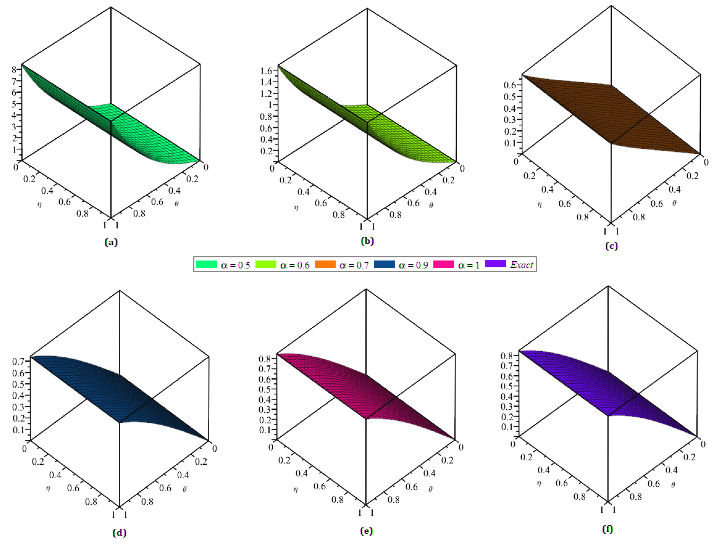
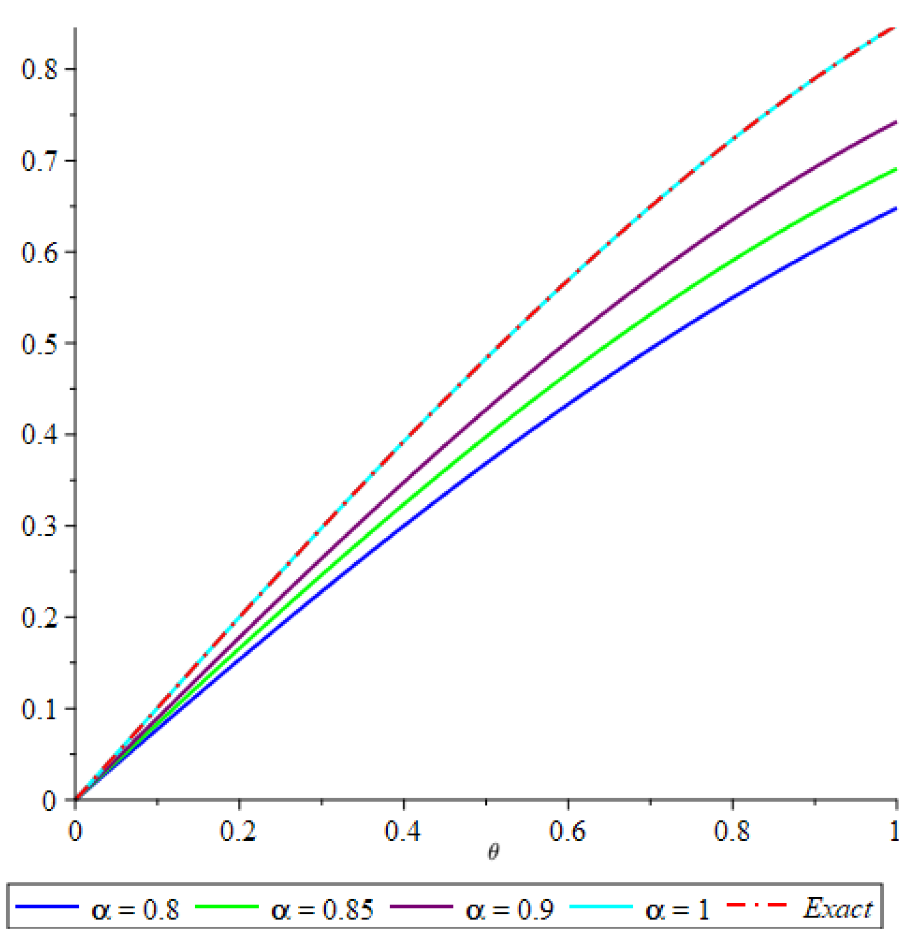
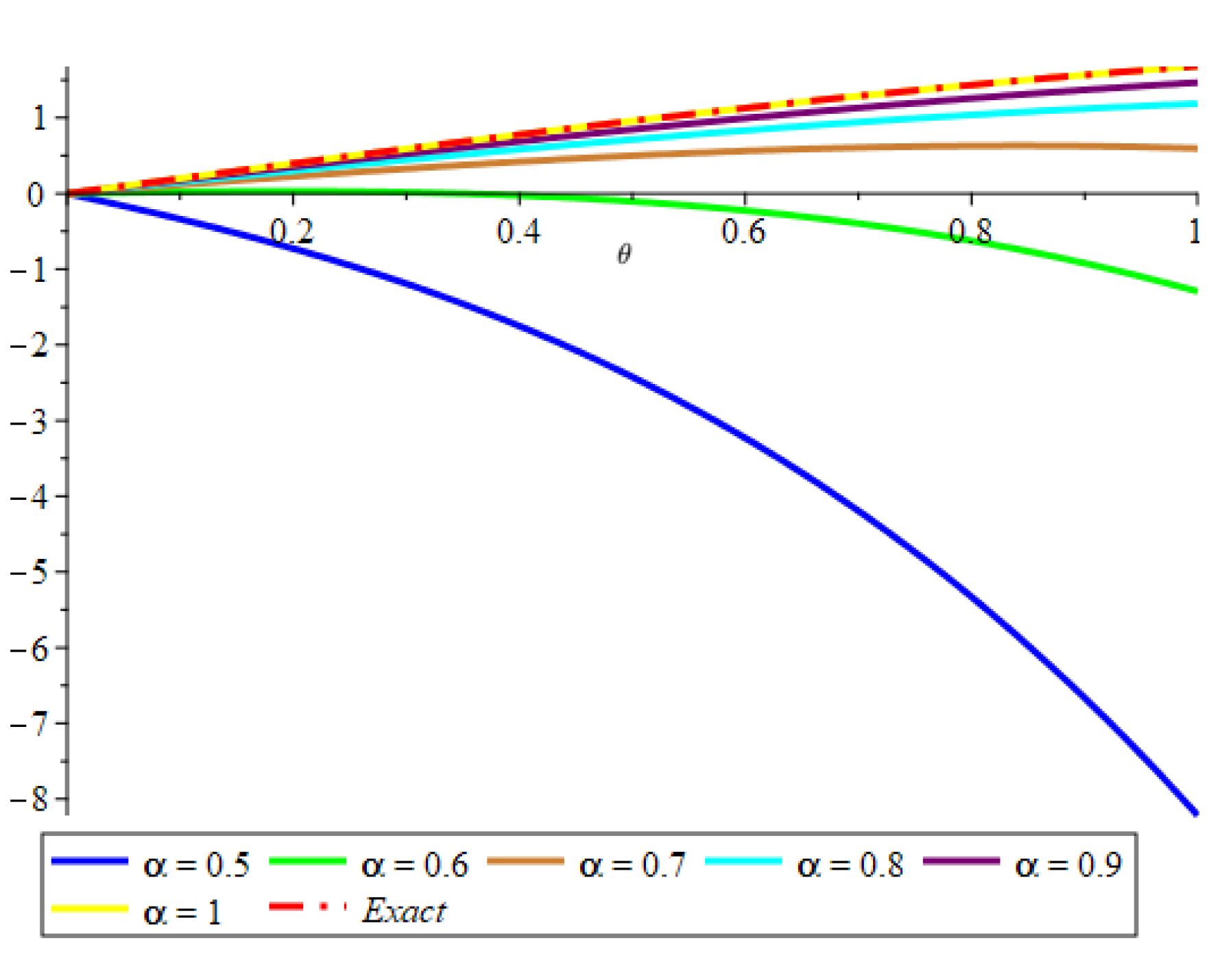
Figure 1, three dimensional graphs of Section 4.1 at (a) , (b) , (c) , (d) , (e) , and (f) Exact. Figure 2, two dimensional plots of the Section 4.1 for various values of . Table 1, absolute error (AE) at , and various fractional order absolute error (AE) at , and various fractional order.
4.2. Problem
Consider the fractional-order two-dimensional parabolic equation [34]:
with initial conditions
with boundary conditions
Taking AT on Equation (34) and then using Equation (35), we obtain
The non-linear operator is presented with the help of future algorithm as below
The deformation equation of m-th order with the help of at , is given by
where
Using inverse Aboodh transform on Equation (39), it reduces to
Using initial conditions to simplify the above equation, we can find the terms of the series solution as
The series solution is given by
Putting the values of in Equation (43), we have
Substituting , and , we obtain
which is the exact solution of Equation (34).
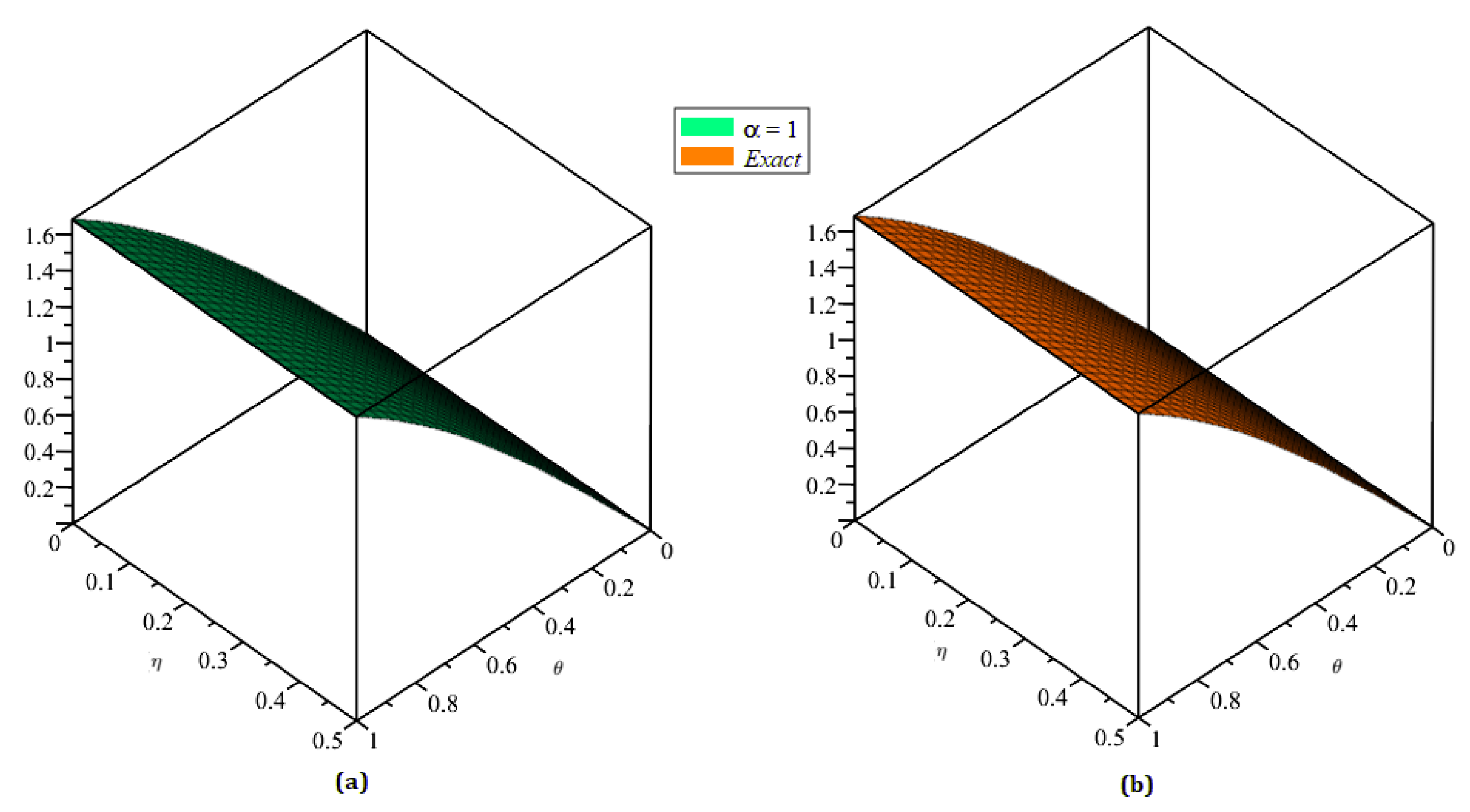
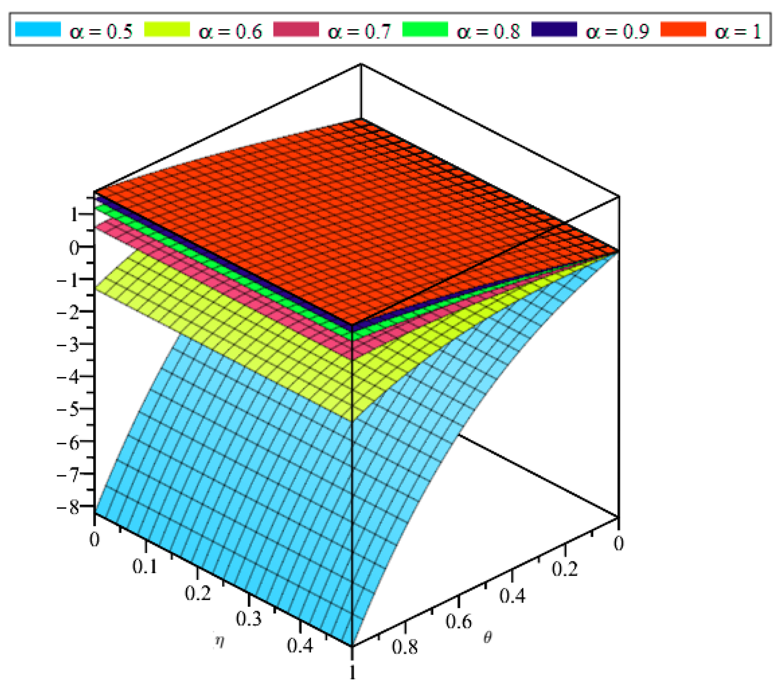
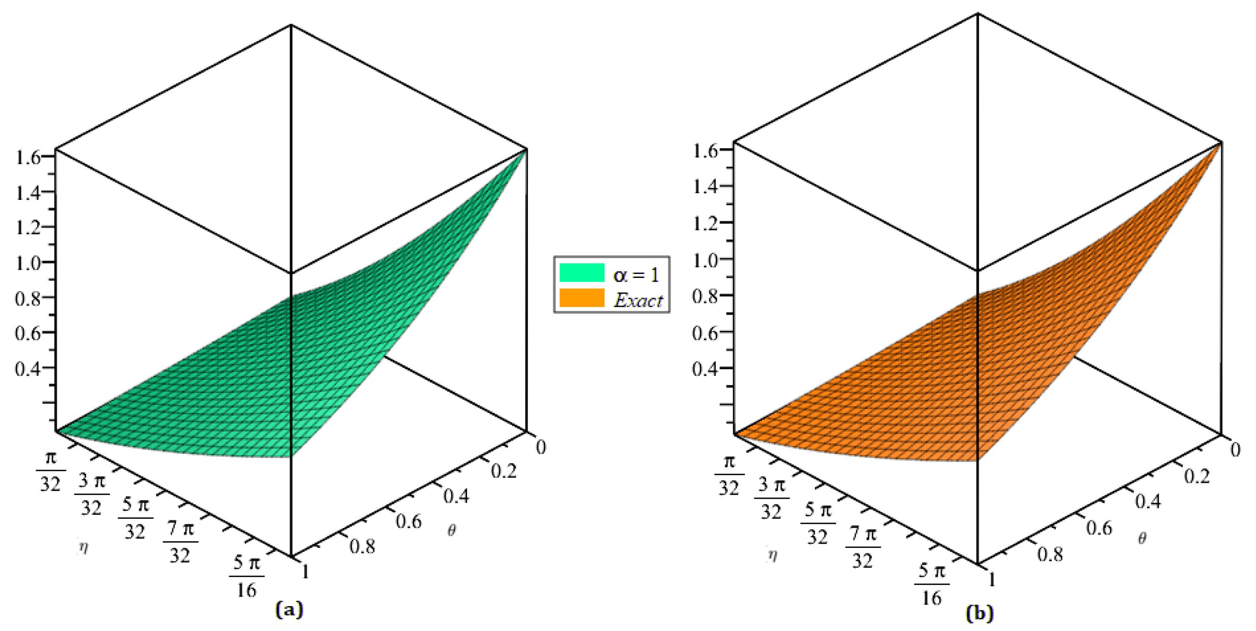
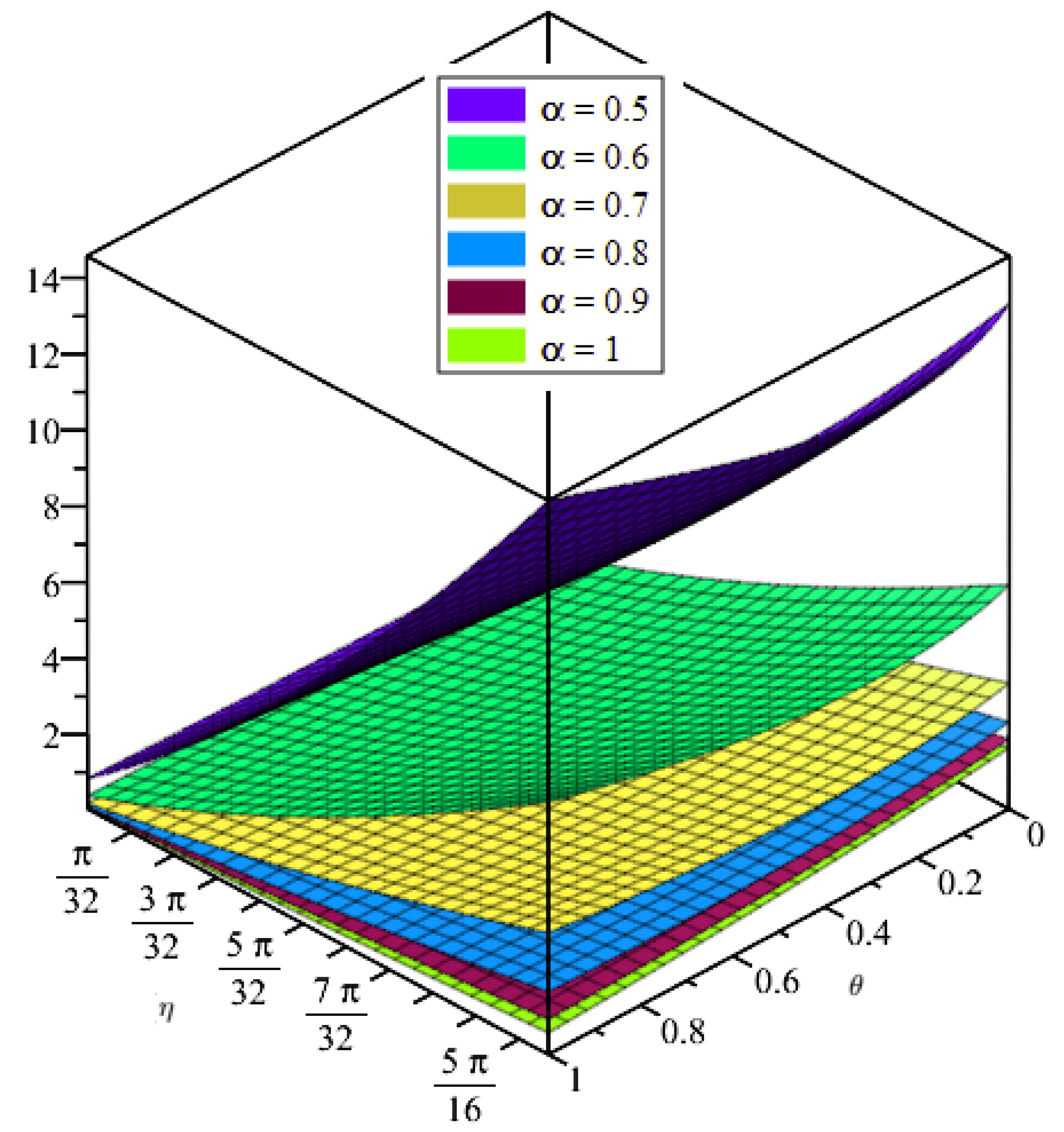
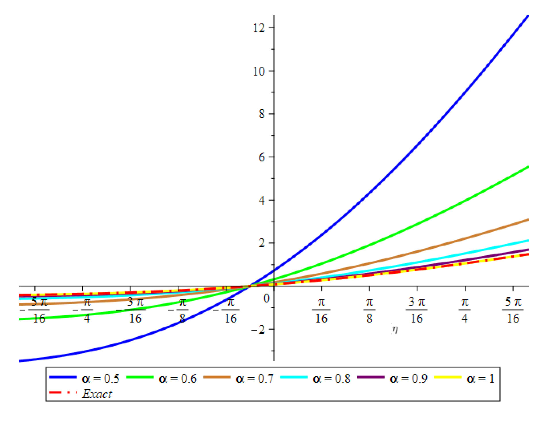
Figure 3, three dimensional graphs of q-HATM solution at (a) and (b) exact Section 4.2. Figure 4, three dimensional graphs of Section 4.2 for different values of . Figure 5, two dimensional plots of the Section 4.2 for various values of and Exact solution. Table 2, absolute error (AE) at , and various fractional order of Section 4.2.
4.3. Problem
Consider the fractional-order two-dimensional parabolic equation [34]:
with initial conditions
with boundary conditions
Using Aboodh tranform on Equation (46) and then applying Equation (47), we obtain
The nonlinear function is represented with the aid of future method as below
The deformation equation of m-th order with the help of at , is given by
where
Applying inverse AT on Equation (51), it reduces to
Using initial conditions to simplify the above equation, we can find the terms of the series solution as
The series solution is given by
Putting the values of in Equation (55), we have
Figure 6, three dimensional graphs of q-HATM solution at (a) and (b) exact Section 4.3. Figure 7, three dimensional graphs of Section 4.3 for different values of . Figure 8, two dimensional plots of the Section 4.3 for various values of and Exact solution.
5. Conclusions
In this study, the q-homotopy analysis transform method is successfully employed to solve fractional parabolic equations numerically. The collected findings indicate the method’s dependability and simplicity. The parameter h provided by the proposed approach allows us to regulate the convergence zone of the series solution. As the q-homotopy analysis transform approach does not require linearization, tiny perturbations, or discretization, computations are drastically reduced. Compared to other methods, the q-homotopy analysis transform method is a competent instrument for obtaining numerical solutions to linked nonlinear fractional partial differential equations.
Funding
This research received no external funding.
Data Availability Statement
The numerical data used to support the findings of this study are included within the article.
Conflicts of Interest
The author declares that there are no conflict of interest regarding the publication of this article.
References
- Nikan, O.; Golbabai, A.; Machado, J.A.; Nikazad, T. Numerical approximation of the time fractional cable model arising in neuronal dynamics. Eng. Comput. 2020, 38, 1–19. [Google Scholar] [CrossRef]
- Oderinu, R.A.; Owolabi, J.A.; Taiwo, M. Approximate solutions of linear time-fractional differential equations. J. Math. Comput. Sci. 2023, 29, 60–72. [Google Scholar] [CrossRef]
- Salama, F.M.; Ali, N.H.M.; Abd Hamid, N.N. Fast O (N) hybrid Laplace transform-finite difference method in solving 2D time fractional diffusion equation. J. Math. Comput. Sci. 2021, 23, 110–123. [Google Scholar] [CrossRef]
- Liouville, J. Memoire surquelques questions de geometrieet de mecanique, et sur un nouveau genre de calcul pour resoudreces questions. J. Ecole Polytech 1832, 13, 1–69. [Google Scholar]
- Riemann, B. Versuch Einer Allgemeinen Auffassung der Integration und Differentiation, Gesammelte Mathematische Werke; Cambridge University Press: Leipzig, Germany, 1896; pp. 1–353. [Google Scholar]
- Caputo, M. Elasticita e Dissipazione; Zanichelli: Bologna, Italy, 1969; pp. 1–300. [Google Scholar]
- Kovalnogov, V.N.; Fedorov, R.V.; Karpukhina, T.V.; Simos, T.E.; Tsitouras, C. Runge-Kutta Embedded Methods of Orders 8(7) for Use in Quadruple Precision Computations. Mathematics 2022, 10, 3247. [Google Scholar] [CrossRef]
- Li, X.; Dong, Z.; Wang, L.; Niu, X.; Yamaguchi, H.; Li, D.; Yu, P. A magnetic field coupling fractional step lattice Boltzmann model for the complex interfacial behavior in magnetic multiphase flows. Appl. Math. Model. 2023, 117, 219–250. [Google Scholar] [CrossRef]
- Jin, H.; Wang, Z.; Wu, L. Global dynamics of a three-species spatial food chain model. J. Differ. Equ. 2022, 333, 144–183. [Google Scholar] [CrossRef]
- Liu, L.; Zhang, S.; Zhang, L.; Pan, G.; Yu, J. Multi-UUV Maneuvering Counter-Game for Dynamic Target Scenario Based on Fractional-Order Recurrent Neural Network. IEEE Trans. Cybern. 2022, 1–14. [Google Scholar] [CrossRef]
- Miller, K.S.; Ross, B. An Introduction to Fractional Calculus and Fractional Differential Equations; A Wiley: New York, NY, USA, 1993; pp. 1–376. [Google Scholar]
- Podlubny, I. Fractional Differential Equations; Academic Press: New York, NY, USA, 1999; pp. 1–366. [Google Scholar]
- Kilbas, A.A.; Srivastava, H.M.; Trujillo, J.J. Theory and Applications of Fractional Differential Equations; Elsevier: Amsterdam, The Netherlands, 2006; pp. 1–541. [Google Scholar]
- Alderremy, A.A.; Iqbal, N.; Aly, S.; Nonlaopon, K. Fractional Series Solution Construction for Nonlinear Fractional Reaction-Diffusion Brusselator Model Utilizing Laplace Residual Power Series. Symmetry 2022, 14, 1944. [Google Scholar] [CrossRef]
- Botmart, T.; Naeem, M.; Iqbal, N. Fractional View Analysis of Emden-Fowler Equations with the Help of Analytical Method. Symmetry 2022, 14, 2168. [Google Scholar] [CrossRef]
- Baleanu, D.; Guvenc, Z.B.; Machado, J.A.T. New Trends in Nanotechnology and Fractional Calculus Applications; Springer: Berlin/Heidelberg, Germany, 2010; pp. 1–544. [Google Scholar]
- Veeresha, P.; Prakasha, D.G.; Baskonus, H.M. Solving smoking epidemic model of fractional order using a modified homotopy analysis transform method. Math. Sci. 2019, 13, 115–128. [Google Scholar] [CrossRef]
- Veeresha, P.; Prakasha, D.G.; Baskonus, H.M. New numerical surfaces to the mathematical model of cancer chemotherapy effect in Caputo fractional derivatives. Chaos 2019, 2, 013119. [Google Scholar] [CrossRef]
- Yasmin, H.; Iqbal, N. A comparative study of the fractional coupled burgers and Hirota-Satsuma KdV equations via analytical techniques. Symmetry 2022, 14, 1364. [Google Scholar] [CrossRef]
- Prakasha, D.G.; Veeresha, P.; Baskonus, H.M. Analysis of the dynamics of hepatitis E virus using the Atangana–Baleanu fractional derivative. Eur. Phys. J. Plus 2019, 134, 1–11. [Google Scholar] [CrossRef]
- Veeresha, P.; Prakasha, D.G.; Baleanu, D. An efficient numerical technique for the nonlinear fractional Kolmogorov-Petrovskii-Piskunov equation. Mathematics 2019, 7, 265. [Google Scholar] [CrossRef] [Green Version]
- Liao, S.J. Homotopy analysis method: A new analytic method for nonlinear problems. Appl. Math. Mech. 1998, 19, 957–962. [Google Scholar]
- Caputo, M.; Fabrizio, M. A new definition of fractional derivative without singular kernel. Prog. Fract. Differ. Appl. 2015, 1, 73–85. [Google Scholar]
- Atangana, A.; Baleanu, D. New fractional derivatives with nonlocal and non-singular kernel theory and application to heat transfer model. Therm. Sci. 2016, 20, 763–769. [Google Scholar] [CrossRef] [Green Version]
- Khaliq, A.Q.M.; Twizell, E.H. A family of second order methods for variable coefficient fourth order parabolic partial differential equations. Int. J. Comput. Math. 1987, 23, 63–76. [Google Scholar] [CrossRef]
- Mukhtar, S.; Noor, S. The Numerical Investigation of a Fractional-Order Multi-Dimensional Model of Navier-Stokes Equation via Novel Techniques. Symmetry 2022, 14, 1102. [Google Scholar] [CrossRef]
- Andrade, C.; McKee, S. High accuracy ADI methods for fourth order parabolic equations with variable coefficients. J. Comput. Appl. Math. 1977, 3, 11–14. [Google Scholar] [CrossRef] [Green Version]
- Conte, S.D. A stable implicit finite difference approximation to a fourth order parabolic equation. J. ACM 1957, 4, 18–23. [Google Scholar] [CrossRef]
- Royster, W.C.; Conte, S.D. Convergence of finite difference solutions to a solution of the equation of the vibrating rod. Proc. Am. Math. Soc. USA 1956, 7, 742–749. [Google Scholar] [CrossRef]
- Evans, D.J. A stable explicit method for the finite-difference solution of a fourthorder parabolic partial differential equation. Comput. J. 1965, 8, 280–287. [Google Scholar] [CrossRef] [Green Version]
- Evans, D.J.; Yousif, W.S. A note on solving the fourth order parabolic equation by the AGE method. Int. J. Comput. Math. 1991, 40, 93–97. [Google Scholar] [CrossRef]
- Cattani, C.; Rushchitskii, Y. Cubically nonlinear elastic waves: Wave equations and methods of analysis. Int. Appl. Mech. 2003, 39, 1115–1145. [Google Scholar] [CrossRef]
- Prakash, A.; Goyal, M.; Gupta, S. A reliable algorithm for fractional Bloch model arising in magnetic resonance imaging. Pramana 2019, 92, 18. [Google Scholar] [CrossRef]
- Naeem, M.; Azhar, O.F.; Zidan, A.M.; Nonlaopon, K.; Shah, R. Numerical analysis of fractional-order parabolic equations via Elzaki transform. J. Funct. Spaces 2021, 2021, 3484482. [Google Scholar] [CrossRef]
Figure 1.
3D graphs of Section 4.1 at (a) , (b) , (c) , (d) , (e) , and (f) Exact.
Figure 1.
3D graphs of Section 4.1 at (a) , (b) , (c) , (d) , (e) , and (f) Exact.

Figure 2.
Tow dimensional plots of the Section 4.1 for various values of .
Figure 2.
Tow dimensional plots of the Section 4.1 for various values of .

Figure 3.
3D graphs of q-HATM solution at (a) and (b) exact Section 4.2.
Figure 3.
3D graphs of q-HATM solution at (a) and (b) exact Section 4.2.

Figure 4.
3D graphs of Section 4.2 for different values of .
Figure 4.
3D graphs of Section 4.2 for different values of .

Figure 5.
2D plots of the Section 4.2 for various values of and Exact solution.
Figure 5.
2D plots of the Section 4.2 for various values of and Exact solution.

Figure 6.
3D graphs of q-HATM solution at (a) and (b) exact Section 4.3.
Figure 6.
3D graphs of q-HATM solution at (a) and (b) exact Section 4.3.

Figure 7.
3D graphs of Section 4.3 for different values of .
Figure 7.
3D graphs of Section 4.3 for different values of .

Figure 8.
2D plots of the Section 4.3 for various values of and Exact solution.
Figure 8.
2D plots of the Section 4.3 for various values of and Exact solution.


Table 1.
Absolute error (AE) at , and various fractional orders.
| AE () | AE () | AE () | AE () | ||
|---|---|---|---|---|---|
| 0.1 | 1 | 0.01012218412 | 0.03251045834 | 0.01102023356 | 1.0 |
| 2 | 0.0127154723 | 0.04083958402 | 0.0138435992 | 1.0 | |
| 3 | 0.0303665632 | 0.0975313750 | 0.0330607006 | 1.0 | |
| 4 | 0.0957006955 | 0.3073716060 | 0.1041912988 | 3.0 | |
| 5 | 0.271458714 | 0.871871383 | 0.295542627 | 1.0 |
Table 2.
Absolute error (AE) at , and various fractional order of Section 4.2.
Table 2.
Absolute error (AE) at , and various fractional order of Section 4.2.
| AE () | AE () | AE () | AE () | ||
|---|---|---|---|---|---|
| 0.1 | 0.1 | 0.1781757909 | 0.0847577008 | 0.0220435308 | 2.0 |
| 0.2 | 0.1781757987 | 0.0847577046 | 0.0220435318 | 2.0 | |
| 0.3 | 0.1781758810 | 0.0847577437 | 0.0220435419 | 2.0 | |
| 0.4 | 0.1781762972 | 0.0847579415 | 0.0220435931 | 2.0 | |
| 0.5 | 0.1781777226 | 0.0847586190 | 0.0220437685 | 2.0 |
Disclaimer/Publisher’s Note: The statements, opinions and data contained in all publications are solely those of the individual author(s) and contributor(s) and not of MDPI and/or the editor(s). MDPI and/or the editor(s) disclaim responsibility for any injury to people or property resulting from any ideas, methods, instructions or products referred to in the content. |
© 2023 by the author. Licensee MDPI, Basel, Switzerland. This article is an open access article distributed under the terms and conditions of the Creative Commons Attribution (CC BY) license (https://creativecommons.org/licenses/by/4.0/).
Share and Cite
MDPI and ACS Style
Alesemi, M. Numerical Analysis of Fractional-Order Parabolic Equation Involving Atangana–Baleanu Derivative. Symmetry 2023, 15, 237. https://doi.org/10.3390/sym15010237
AMA Style
Alesemi M. Numerical Analysis of Fractional-Order Parabolic Equation Involving Atangana–Baleanu Derivative. Symmetry. 2023; 15(1):237. https://doi.org/10.3390/sym15010237
Chicago/Turabian StyleAlesemi, Meshari. 2023. "Numerical Analysis of Fractional-Order Parabolic Equation Involving Atangana–Baleanu Derivative" Symmetry 15, no. 1: 237. https://doi.org/10.3390/sym15010237
Note that from the first issue of 2016, this journal uses article numbers instead of page numbers. See further details here.