Article

On New Symmetric Schur Functions Associated with Integral and Integro-Differential Functional Expressions in a Complex Domain

by
Samir B. Hadid
1,2 and
Rabha W. Ibrahim
3,4,*
1
Department of Mathematics and Sciences, College of Humanities and Sciences, Ajman University, Ajman P.O. Box 346, United Arab Emirates
2
Nonlinear Dynamics Research Center (NDRC), Ajman University, Ajman P.O. Box 346, United Arab Emirates
3
Mathematics Research Center, Department of Mathematics, Near East University, Near East Boulevard, 99138 Nicosia, Turkey
4
Department of Computer Science and Mathematics, Lebanese American University, Beirut 13-5053, Lebanon
*
Author to whom correspondence should be addressed.
Symmetry 2023, 15(1), 235; https://doi.org/10.3390/sym15010235
Submission received: 15 December 2022 / Revised: 25 December 2022 / Accepted: 3 January 2023 / Published: 14 January 2023
(This article belongs to the Special Issue Symmetry in Mathematical Functional Equations)

Abstract

:
The symmetric Schur process has many different types of formals, such as the functional differential, functional integral, and special functional processes based on special functions. In this effort, the normalized symmetric Schur process (NSSP) is defined and then used to determine the geometric and symmetric interpretations of mathematical expressions in a complex symmetric domain (the open unit disk). To obtain more symmetric properties involving NSSP, we consider a symmetric differential operator. The outcome is a symmetric convoluted operator. Geometrically, studies are presented for the suggested operator. Our method is based on the theory of differential subordination.

1. Introduction and Preliminaries

The class of analytic functions from the open unit disk to its closure are what make-up the symmetric Schur functions. These functions, along with their matrices and operator-valued variations, are key elements in harmonic analysis, while their relevance extends far beyond complex analyses to a variety of fields, including linear system concepts, signal processing, electrical engineering, stochastic processes, geophysics, functional principles, interpolation issues, the class of polynomials with orthogonality properties on the unit circle, and quantum calculus. The description of these functions by a series of complex factors and the Schur strictures resulting from the so-called Schur process are their key and most advantageous characteristics [1,2]. This process ς is formulated by different types of functional expressions starting from the basic formula, as follows:
ς 0 ( z ) = ϕ ( z ) ς k ( z ) = z 1 ϕ ( z ) ϕ ( 0 ) z ϕ ( z ) ϕ ( z ) ϕ ( 0 ) , k N ,
where ϕ is analytic at the origin. The modified process is presented by using the Möbius transformation [3]
ς 0 ( z ) = ϕ ( z ) ς k ( z ) = z 1 ϕ ( z ) ε k 1 ε k ¯ ϕ ( z ) , k N .
Moreover, it can be suggested by some functional integrals, such as the Stieltjes function, Nevanlinna function, and Carathéodory function [2].
In this work, the normalized symmetric Schur process (NSSP) is introduced by using a functional integral and utilized to interpret mathematical expressions in a complex symmetric domain in terms of geometry functional formula in the open unit disk. The Fekete–Szegö problem (for specific subclasses of starlike univalent functions) is considered based on the proposed convoluted operator. This problem was studied recently in [4].
The class of normalized analytic functions Ξ admits the following power series
ϕ ( z ) = z + n = 2 ϕ n z n , z Δ : = { z C : | z | < 1 } ,
where ϕ n , n = 2 , 3 , 4 , represent the coefficients of the analytic function ϕ ( z ) , satisfying the equality ϕ ( 0 ) = 0 = ϕ ( 0 ) 1 .
Two functions ϕ and φ in Ξ are convoluted if and only if
ϕ ( z ) φ ( z ) = z + n = 2 ϕ n φ n z n , z Δ ,
where
φ ( z ) = z + n = 2 φ n z n , z Δ ,
such that φ n , n = 2 , 3 , 4 , indicate the coefficients of the analytic function φ ( z ) .
We take into account symmetric integral operators to obtain additional symmetric features involving NSSP. A symmetric convoluted operator is the result. Studies in geometry are provided for the proposed operator. Our approach is created by the differential subordination scheme. Two analytic functions ϕ and φ are subordinated ( ϕ φ ) if the analytic function σ in Δ with σ ( 0 ) = 0 and | σ ( z ) | < 1 occur, such that
ϕ ( z ) = φ ( σ ( z ) ) , z Δ .
Additionally, the following equivalence holds if the function φ is univalent in Δ :
ϕ ( z ) φ ( z ) ϕ ( 0 ) = φ ( 0 ) , ϕ ( Δ ) φ ( Δ ) .
The rest of the paper is as follows: Section 2 deals with the suggested NSSP; Section 3 includes the main results involving the suggested NSSP, and Section 4 presents the conclusion and future works.

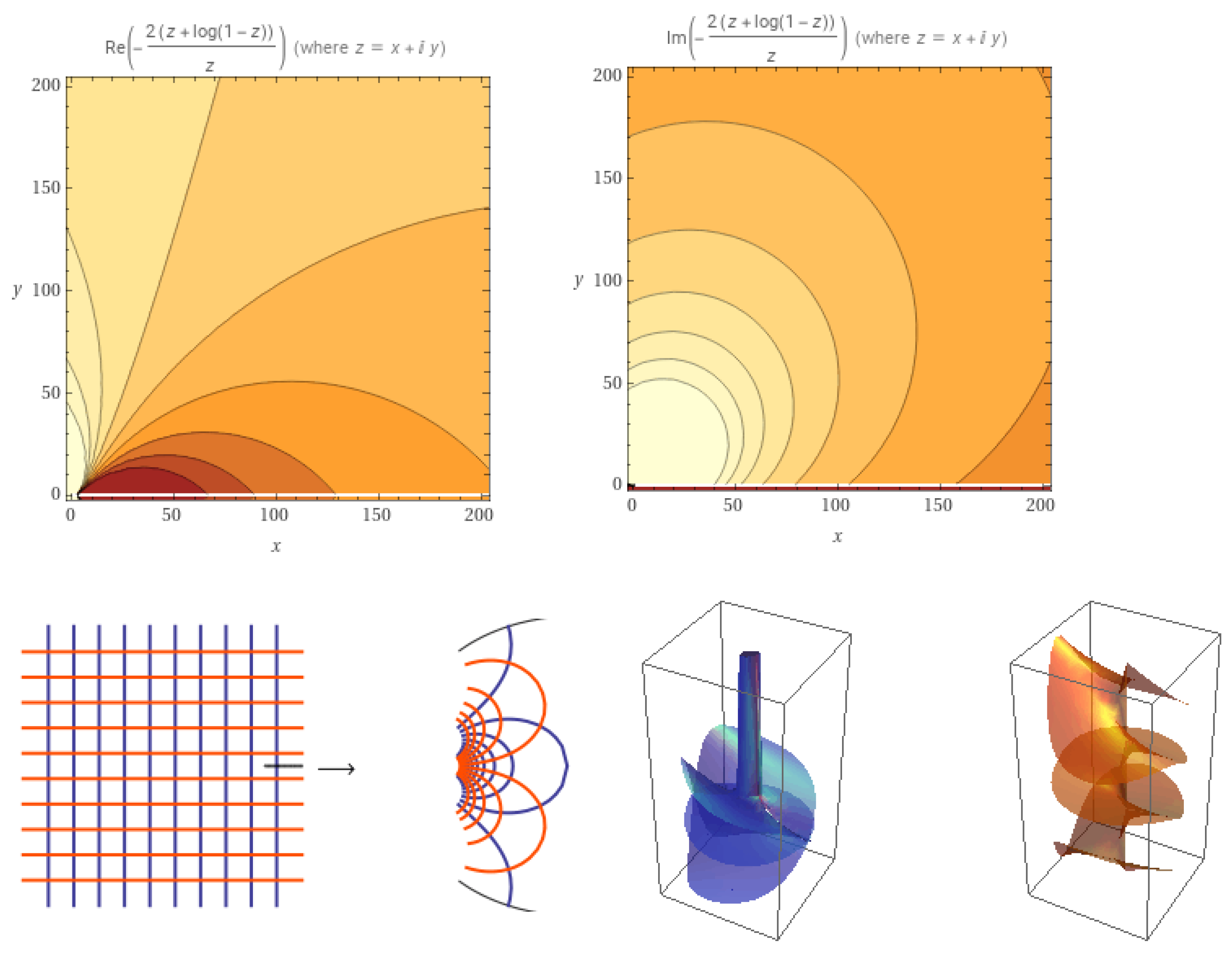
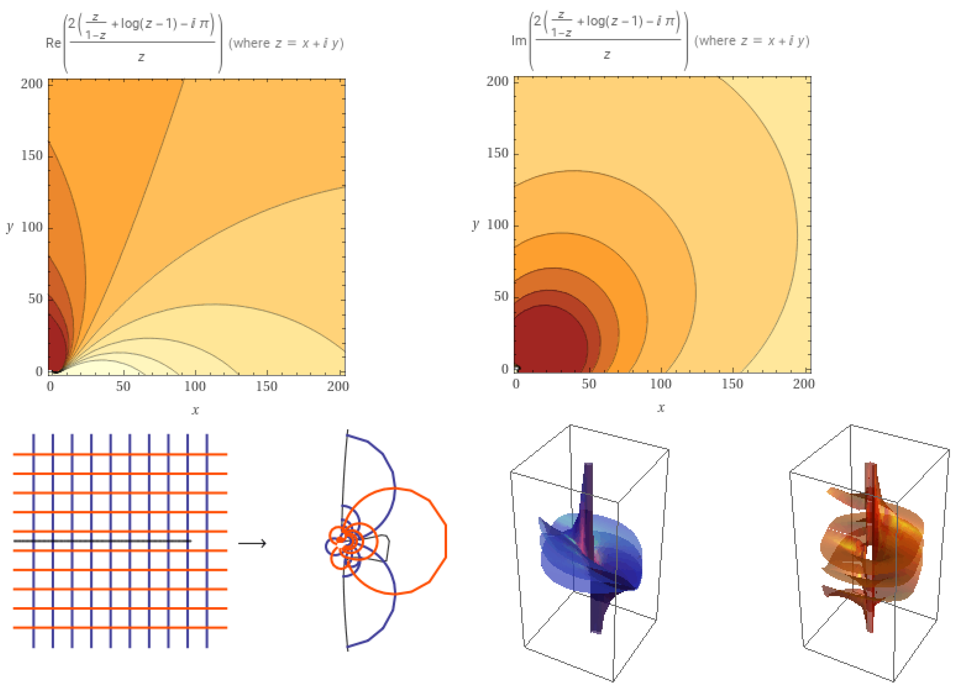
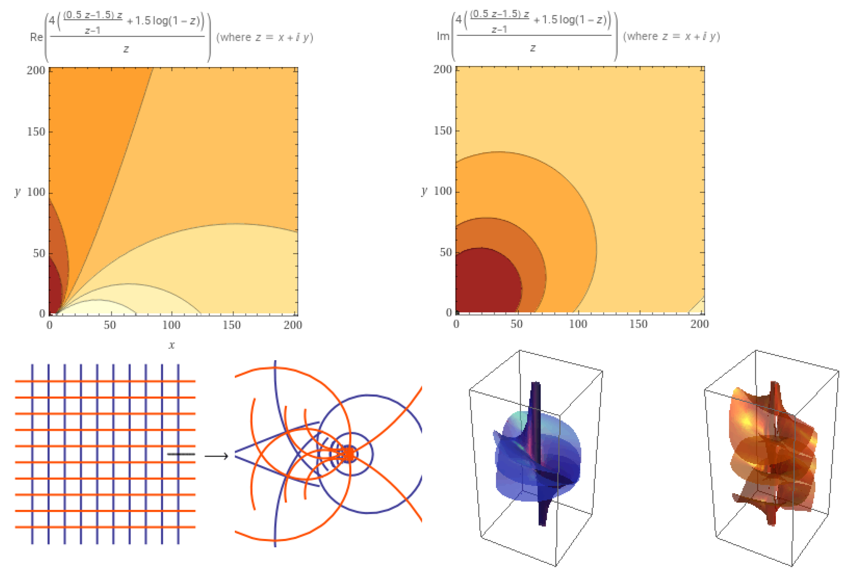
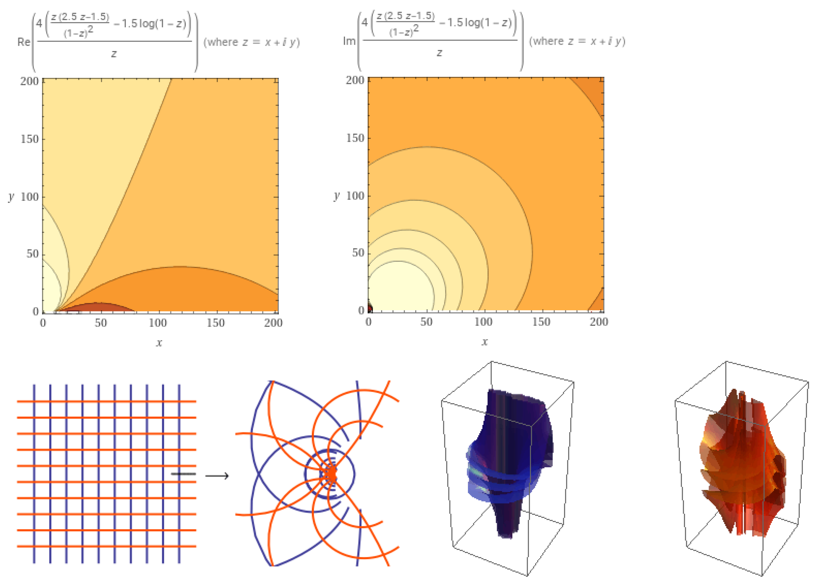
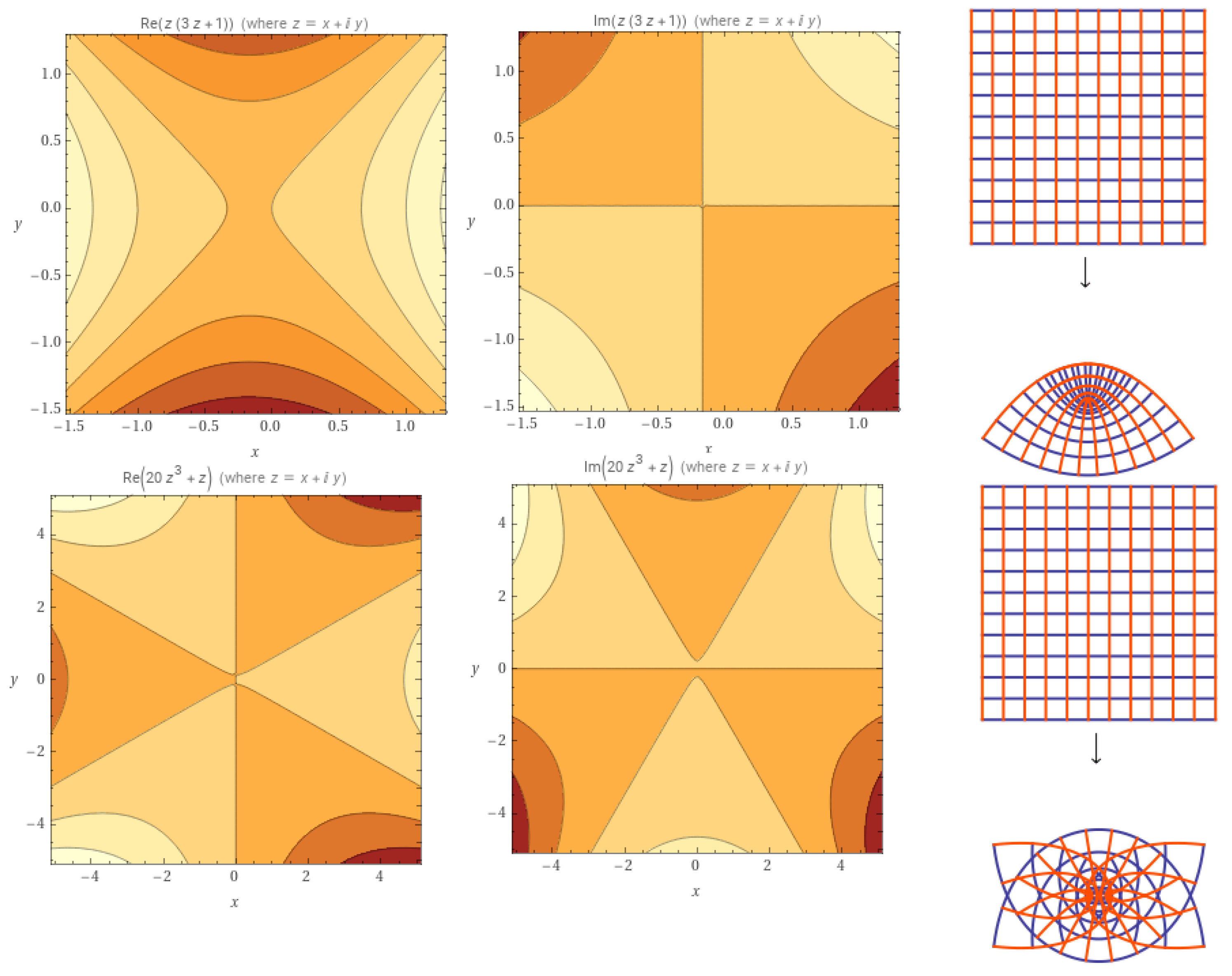
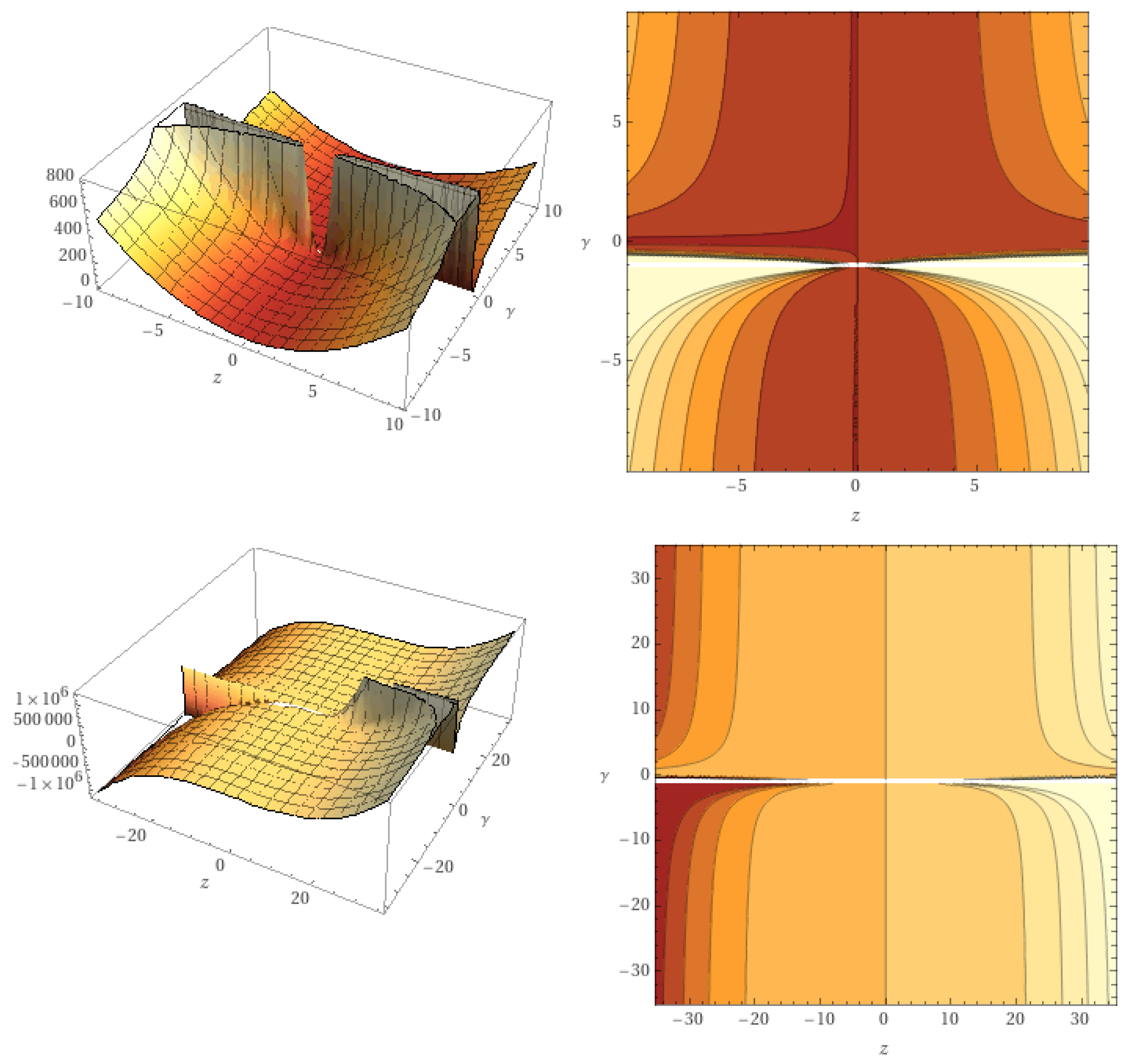
2. The Iteration of NSSP

The process NSSP is suggested in terms of functional integrals, as follows: for a normalized function ϕ Ξ , the process is defined by the iteration
ς 0 ( z ) = ϕ ( z ) = z + n = 2 ϕ n z n ς 1 ( z ) = z 1 2 0 z ς 0 ( w ) d w = 2 z 1 z 2 2 + n = 2 ϕ n z n + 1 n + 1 = z + n = 2 2 n + 1 ϕ n z n ; ς 2 ( z ) = z 1 2 0 z ς 1 ( w ) d w = 2 z 1 z 2 2 + n = 2 ϕ n 2 n + 1 z n + 1 n + 1 = z + n = 2 2 n + 1 2 ϕ n z n ; ς k ( z ) = z 1 2 0 z ς k 1 ( w ) d w = 2 z 1 z 2 2 + n = 2 ϕ n 2 n + 1 k 1 z n + 1 n + 1
= z + n = 2 2 n + 1 k ϕ n z n .
It is clear that ς k Ξ .
For example, let ϕ ( z ) = z 1 z , then (see Figure 1)
ς ( z ) = ( 2 ( z log ( 1 z ) ) ) z = z + 2 z 2 3 + z 3 2 + 2 z 4 5 + z 5 3 + 2 z 6 7 + O ( z 7 ) .
Moreover, let ϕ ( z ) = z ( 1 z ) 2 then (see Figure 2)
ς ( z ) = ( 2 ( 1 / ( 1 z ) + log ( z 1 ) i π 1 ) z = z + 4 z 2 3 + 3 z 3 2 + 8 z 4 5 + 5 z 5 3 + O ( z 6 ) .
Note that for k > 1
n = 1 2 n + 1 k = 2 k ( ζ ( k ) 1 ) ,
where ζ indicates the Riemann–Zeta function. Moreover, for k > 1 , the second sum is converge as follows:
n = 2 2 n + 1 k = 2 k ζ ( k , 3 ) ,
where ζ indicates the generalized Riemann–Zeta function. Moreover, NSSP satisfies the convoluted product
ς k ( z ) = z + n = 2 ϕ n z n z + n = 2 2 n + 1 k z n : = ϕ ( z ) k ( z ) = z + n = 2 φ n z n .
Another new formula is given as an integro-differential expression, as follows:
ð 0 ( z ) = ϕ ( z ) = z + n = 2 ϕ n z n ð 1 γ ( z ) = 2 γ z 1 0 z [ w ð 0 ( w ) ( 1 γ ) ð 0 ( w ) ] d w = z + n = 2 2 n ( 1 γ ) γ ( n + 1 ) ϕ n z n ; ð 2 γ ( z ) = 2 γ z 1 0 z ð 1 ( w ) d w = z + n = 2 2 n ( 1 γ ) γ ( n + 1 ) 2 ϕ n z n ; ð k γ ( z ) = 2 γ z 1 0 z ð k 1 ( w ) d w = z + n = 2 2 n ( 1 γ ) γ ( n + 1 ) k ϕ n z n , γ ( 0 , 1 ] = z + n = 2 ϕ n z n z + n = 2 2 n ( 1 γ ) γ ( n + 1 ) k z n : = ϕ ( z ) P k γ ( z ) .
Thus,
ð k γ ( z ) = z + n = 2 υ n z n .
It is clear that ð k γ Ξ . The boundedness of the expression z 1 [ z ð 0 ( z ) ( 1 γ ) ð 0 ( z ) ] implies the boundedness of ð 0 ( z ) = ϕ ( z ) (see Theorem 1 of [5]). Moreover, it is a univalent starlike of the order 1 γ (Theorem 2 of [5]). Table 1 shows the convergence of the coefficients of the function P k γ ( z ) , in terms of special functions, where γ indicates the Euler–Mascheroni constant, I is the modified Bessel function of the first kind, and ψ is the polygamma function and the generalized hypergeometric function.
For example, let ϕ ( z ) = z / ( 1 z ) , then for k = 1 , γ = 0.5 the process becomes (see Figure 3)
ð 1 0.5 ( z ) = 4 ( ( 0.5 z 1.5 ) z ) ( z 1 ) + 1.5 log ( 1 z ) z , ( z ) 0.99999
= z + 2 z 2 + 2.5 z 3 + 2.8 z 4 + 3 z 5 + O ( z 6 ) .
Moreover, for ϕ ( z ) = z / ( 1 z ) 2 , we have (see Figure 4)
ð 1 0.5 ( z ) = 4 ( ( 2.5 z 1.5 ) z ) ( z 1 ) 2 1.5 log ( 1 z ) z , ( z ) 0.99999
= z + 4 z 2 + 7.5 z 3 + 11.2 z 4 + 15 z 5 + 18.8571 z 6 + O ( z 7 ) , | z | < 1

3. Results

We aim to explore more properties of the NSSP.
Theorem 1.
Suppose that the NSSP: ς k ( z ) satisfies the inequality
z ς k ( z ) ς k ( z ) 1 + u z 1 + v z , v [ 1 , u ) , u ( v , 1 ] .
Then
| ϕ 2 | u v ( 2 / 3 ) k ;
and
| ϕ 3 | 18 k ( v + 1 ) 2 + u v ( 2 / 3 ) k 2 8 k 2 × 9 k .
Moreover, for ρ : = 2 k 3 ( 1 v ) , the Fekete–Szegö functional becomes
ϕ 3 τ ϕ 2 2 ρ max 1 , 2 2 k ( 3 2 k τ ( 2 v 2 + 4 v 2 ) 2 2 k + 2 2 k + 1 ( v 2 3 v ) )
when τ C . Moreover,
ϕ 3 τ ϕ 2 2 ρ 2 ( 2 1 2 k 3 2 k τ ( v 1 ) 2 2 v 2 + 6 v + 1 ) i f τ < ( v 3 2 + 11 2 ) ( v 3 2 11 2 ) 2 1 2 k 3 2 k ( v 1 ) 2 2 k 2 ( 1 v ) i f 0 τ 1 2 ( 2 1 2 k 3 2 k τ ( v 1 ) 2 2 v 2 + 6 v + 1 ) i f τ > ( v 3 2 + 3 ) ( v 3 2 3 ) 2 2 2 k 3 2 k ( v 1 ) 2
when τ R .
Proof. 
The subordination inequality implies the functional formula
z ς k ( z ) ς k ( z ) = ( u + 1 ) h ( z ) ( u 1 ) ( v + 1 ) h ( z ) ( v 1 ) ,
where h ( z ) = 1 + h 1 z + h 2 z 2 + such that ( h ( z ) ) > 0 . A computation yields that
( u + 1 ) h ( z ) ( u 1 ) ( v + 1 ) h ( z ) ( v 1 ) = 1 + 1 2 h 1 z ( u v ) 1 4 z 2 ( ( h 1 2 ( v + 1 ) 2 h 2 ) ( u v ) ) + 1 8 h 1 ( v + 1 ) z 3 ( h 1 2 ( v + 1 ) 4 h 2 ) ( u v ) 1 16 z 4 ( ( v + 1 ) ( h 1 4 ( v + 1 ) 2 6 h 2 h 1 2 ( v + 1 ) + 4 h 2 2 ) ( u v ) ) + O ( z 5 ) .
On the other hand, we have
z ς k ( z ) ς k ( z ) = 1 + ϕ 2 ( 2 / 3 ) k z + z 2 ( 2 ϕ 3 9 k ϕ 2 2 8 k ) 18 k + z 3 ϕ 2 3 k ( ϕ 2 2 ( 8 / 9 ) k 3 ϕ 3 ) + z 4 ( ϕ 2 4 ( 64 k ) + ϕ 3 ϕ 2 2 2 ( 3 k + 2 ) 9 k 2 ϕ 3 2 81 k ) 324 k + O ( z 5 )
Comparing the last two qualities, we have
ϕ 2 = ( 1 / 2 ) ( u v ) ( 2 / 3 ) k h 1
and
ϕ 3 = 18 k 4 ( 2 h 2 h 1 2 ( v + 1 ) ) ( u v ) + ( 1 / 2 ) ( u v ) ( 2 / 3 ) k 2 h 1 2 8 k 2 × 9 k .
Since | h i | 2 , , i = 2 , 3 , where ( h ( z ) ) > 0 then
| ϕ 2 | u v ( 2 / 3 ) k ;
and
| ϕ 3 | 18 k ( v + 1 ) 2 + u v ( 2 / 3 ) k 2 8 k 2 × 9 k .
Obviously, we have the equality
ϕ 3 τ ϕ 2 2 = 2 k 3 ( u v ) h 2 κ h 1 2 ,
where
κ : = u v ( 2 / 3 ) k 2 ( 4 9 ) k τ ( v + 1 ) .
In view of the Fekete–Szegö theory, we obtain the last inequalities. □
Theorem 2.
Suppose that the NSSP: ð k γ ( z ) fulfills the inequality
z ( ð k γ ( z ) ) ð k γ ( z ) 1 + u z 1 + v z , v [ 1 , u ) , u ( v , 1 ] .
Then
| ϕ 2 | 3 γ 2 ( γ + 1 ) k ( u v ) ;
and
| ϕ 3 | γ 6 ( γ + 1 ) ) k + 2 k 1 ( u v ) , γ ( 0 , 1 ] .
Moreover, for ρ : = 2 k 3 ( 1 v ) , the Fekete–Szegö functional becomes
υ 3 ϱ υ 2 2 2 k 2 ( u v ) max 1 , 2 1 3 k 9 k | ϱ | 1 + 1 γ 2 k
when ϱ C . Moreover,
υ 3 ϱ υ 2 2 2 k 2 ( u v ) 2 2 3 k 9 k ϱ ( 1 / γ + 1 ) 2 k i f ϱ < 0 2 k 1 ( u v ) i f 0 ϱ 1 2 k 2 ( u v ) 2 2 3 k 9 k ϱ ( 1 / γ + 1 ) 2 k i f ϱ > 0
when ϱ R .
Proof. 
The subordination inequality implies the functional formula
z ( ð k γ ( z ) ) ð k γ ( z ) = ( u + 1 ) g ( z ) ( u 1 ) ( v + 1 ) g ( z ) ( v 1 ) ,
where g ( z ) = 1 + g 1 z + g 2 z 2 + such that ( g ( z ) ) > 0 . A computation yields that
( u + 1 ) g ( z ) ( u 1 ) ( v + 1 ) g ( z ) ( v 1 ) = 1 + 1 2 g 1 z ( u v ) 1 4 z 2 ( ( g 1 2 ( v + 1 ) 2 g 2 ) ( u v ) ) + 1 8 g 1 ( v + 1 ) z 3 ( g 1 2 ( v + 1 ) 4 g 2 ) ( u v ) 1 16 z 4 ( ( v + 1 ) ( g 1 4 ( v + 1 ) 2 6 g 2 g 1 2 ( v + 1 ) + 4 g 2 2 ) ( u v ) ) + O ( z 5 ) .
On the other hand, we have
z ( ð k γ ( z ) ) ð k γ ( z ) = 1 + ϕ 2 ( 2 / 3 ) k z ( 1 + γ γ ) k + 18 k z 2 2 ϕ 3 9 k ( γ + 2 γ ) k ϕ 2 2 8 k ( 1 + γ γ ) 2 k + ϕ 2 3 k z 3 ( 1 + γ γ ) k ϕ 2 2 ( 8 / 9 ) k ( 1 + γ γ ) 2 k 3 ϕ 3 ( γ + 2 γ ) k + 324 k z 4 ϕ 2 2 ϕ 3 2 3 k + 2 9 k ( 1 + γ γ ) 2 k ( γ + 2 γ ) k 2 ϕ 3 2 81 k ( γ + 2 γ ) 2 k ϕ 2 4 64 k ( 1 + γ γ ) 4 k + O ( z 5 )
Comparing the last two qualities, we have
ϕ 2 = ( 1 / 2 ) ( u v ) ( 2 / 3 ) k ( 1 + γ γ ) k g 1
and
ϕ 3 = 2 k 3 2 g 2 σ 1 g 1 2 ( u v ) ,
where σ 1 : = v + 1 2 12 k ( γ γ + 1 ) k . Since | g i | 2 , i = 2 , 3 , where ( g ( z ) ) > 0 then
| ϕ 2 | 3 γ 2 ( γ + 1 ) k ( u v ) ;
and
| ϕ 3 | γ 6 ( γ + 1 ) ) k + 2 k 1 ( u v ) , γ ( 0 , 1 ] .
Furthermore, we have the equality
ϕ 3 ϱ ϕ 2 2 = 2 k 2 ( u v ) g 2 ϵ g 1 2 ,
where
ϵ : = 1 2 + ϱ 4 ( 2 / 3 ) 2 k ( 1 + γ γ ) 2 k 2 k 2
In view of the Fekete–Szegö theory, we obtain the last inequalities. □
In general, we have the following results that describe the upper bound of | ϕ n | .
Theorem 3.
Let
z ς k ( z ) ς k ( z ) 1 + u z 1 + v z , v [ 1 , u ) , u ( v , 1 ] .
Then
| ϕ 2 | λ 3 2 k , | ϕ 3 | λ ( 1 + λ ) 4 2 k ,
and
| ϕ n | λ n + 1 2 k ı = 1 n 2 ( 1 + λ ) ı , n 3 ,
where λ : = max v n 1 ( u + v ) .
Proof. 
It is clear that
1 + u z 1 + v z = 1 + n = 1 ( v ) n ( u + v ) ) v z n .
Moreover, by the definition of ς k ( z ) , we have
z ς k ( z ) ς k ( z ) = z + n = 2 n ϕ n 2 n + 1 k z n z + n = 2 ϕ n 2 n + 1 k z n .
Now there is an analytic function ( z ) in Δ , such that ( 0 ) = 1 satisfies the equation
z ς k ( z ) ς k ( z ) = ( z ) .
In terms of the power series, we have
z + n = 2 n ϕ n 2 n + 1 k z n = z + n = 2 ϕ n 2 n + 1 k z n 1 + n = 1 n z n = n = 2 ϕ n 2 n + 1 k z n n = 0 n z n + n = 0 n z 1 + n .
As a result of comparing the z n coefficients, we now have
n ϕ n 2 n + 1 k ϕ n 2 n + 1 k = j = 1 n 1 ϕ j 2 j + 1 k n j ,
which implies
( n 1 ) ϕ n 2 n + 1 k = j = 1 n 1 ϕ j 2 j + 1 k n j .
Thus,
ϕ n = j = 1 n 1 ϕ j 2 j + 1 k n j ( n 1 ) 2 n + 1 k .
However,
| n | max v n 1 ( u + v ) : = λ ,
then we obtain
| ϕ n | j = 1 n 1 | ϕ j | 2 j + 1 k λ ( n 1 ) 2 n + 1 k j = 1 n 1 | ϕ j | 2 j + 1 k λ 2 n + 1 k .
For n = 2 , we have
| ϕ 2 | j = 1 1 | ϕ j | 2 j + 1 k λ 2 2 + 1 k = λ 3 2 k .
For n = 3 , we have
| ϕ 3 | j = 1 2 | ϕ j | 2 j + 1 k λ 2 4 k λ ( 1 + λ ) 4 2 k .
Consequently, for n = 4 ,
| ϕ 4 | j = 1 3 | ϕ j | 2 j + 1 k λ 2 5 k λ ( 1 + λ ) 2 5 2 k .
Thus, by induction, we have
| ϕ n | λ n + 1 2 k ı = 1 n 2 ( 1 + λ ) ı , n 3 .
Corollary 1.
Let
z ( ς k ( z ) ) ς k ( z ) 1 + u z 1 + v z , v [ 1 , u ) , u ( v , 1 ] .
Then
| ϕ n | λ E 1 , 1 k 1 log ( 2 ) log ( n + 1 ) log ( n + 1 ) ı = 1 n 2 ( 1 + λ ) ı , n 3 ,
where λ = max v n 1 ( u + v ) and E p , q represents the Mittag-Leffler function.
Proof. 
In view of Theorem 3 and by using the power series together with the definition of the Mittag-Leffler function, we conclude from the results
( n + 1 2 ) k = v = 0 k v 1 log ( 2 ) log ( n + 1 ) v log v ( n + 1 ) Γ ( v + 1 ) = E 1 , 1 k 1 log ( 2 ) log ( n + 1 ) log ( n + 1 ) , n = 2 , 3 , .
Similarly, we have the following coefficient bounds of ð k γ .
Theorem 4.
Let
z ( ð k γ ( z ) ) ð k γ ( z ) 1 + u z 1 + v z , v [ 1 , u ) , u ( v , 1 ] .
Then
| ϕ 2 | λ 3 2 k γ γ + 1 k , | ϕ 3 | λ ( 1 + λ ) 4 2 k γ γ + 2 k ,
and
| ϕ n | λ n + 1 2 k γ γ + n 1 k ı = 1 n 2 ( 1 + λ ) ı , n 3 ,
where λ = max v n 1 ( u + v ) .
Proof. 
It is clear that
1 + u z 1 + v z = 1 + n = 1 ( v ) n ( u + v ) ) v z n .
In addition, by the definition of ð k γ ( z ) , we have
z ( ð k γ ( z ) ) ð k γ ( z ) = z + n = 2 n ϕ n 2 n ( 1 γ ) γ ( n + 1 ) k z n z + n = 2 ϕ n 2 n ( 1 γ ) γ ( n + 1 ) k z n .
Now there is the analytic function ( z ) in Δ , such that ( 0 ) = 1 satisfies the equation
z ( ð k γ ( z ) ) ς k ( z ) = ( z ) .
In terms of the power series, we have
z + n = 2 n ϕ n 2 n ( 1 γ ) γ ( n + 1 ) k z n = z + n = 2 ϕ n 2 n ( 1 γ ) γ ( n + 1 ) k z n 1 + n = 1 n z n = n = 2 ϕ n 2 n ( 1 γ ) γ ( n + 1 ) k z n n = 0 n z n + n = 0 n z 1 + n .
As an outcome of comparing the z n coefficients, we then have
n ϕ n 2 n ( 1 γ ) γ ( n + 1 ) k ϕ n 2 n ( 1 γ ) γ ( n + 1 ) k = j = 1 n 1 ϕ j 2 j ( 1 γ ) γ ( j + 1 ) k n j ,
which yields
( n 1 ) ϕ n 2 n ( 1 γ ) γ ( n + 1 ) k = j = 1 n 1 ϕ j 2 j ( 1 γ ) γ ( j + 1 ) k n j .
Thus, we find the next inequality
ϕ n = j = 1 n 1 ϕ j 2 j ( 1 γ ) γ ( j + 1 ) k n j ( n 1 ) 2 n + 1 k .
However,
| n | max v n 1 ( u + v ) = λ ,
then we obtain
| ϕ n | j = 1 n 1 | ϕ j | 2 j ( 1 γ ) γ ( j + 1 ) k λ ( n 1 ) 2 n ( 1 γ ) γ ( n + 1 ) k j = 1 n 1 | ϕ j | 2 j ( 1 γ ) γ ( j + 1 ) k λ 2 n ( 1 γ ) γ ( n + 1 ) k .
For n = 2 , we receive
| ϕ 2 | j = 1 1 | ϕ j | 2 1 ( 1 γ ) 2 γ k λ 2 2 ( 1 γ ) γ ( 2 + 1 ) k = λ 3 2 k γ γ + 1 k .
For n = 3 , we have
| ϕ 3 | j = 1 2 | ϕ j | 2 j ( 1 γ ) γ ( j + 1 ) k λ 2 3 ( 1 γ ) γ ( 3 + 1 ) k λ ( 1 + λ ) 4 2 k γ γ + 2 k .
Consequently, for n = 4 ,
| ϕ 4 | j = 1 3 | ϕ j | 2 j ( 1 γ ) γ ( j + 1 ) k λ 2 n ( 1 γ ) γ ( n + 1 ) k λ ( 1 + λ ) 2 5 2 k γ γ + 3 k .
Thus, by induction, we have
| ϕ n | λ n + 1 2 k γ γ + n 1 k ı = 1 n 2 ( 1 + λ ) ı , n 3 .
Corollary 2.
Let
z ( ð k γ ( z ) ) ð k γ ( z ) 1 + u z 1 + v z , v [ 1 , u ) , u ( v , 1 ] .
Then
| ϕ 2 | λ 3 2 k E 1 , 1 k log γ γ + 1 ,
| ϕ 3 | λ ( 1 + λ ) 4 2 k E 1 , 1 k log γ γ + 2 ,
and
| ϕ n | λ E 1 , 1 k 1 log ( 2 ) log ( n + 1 ) log ( n + 1 ) × E 1 , 1 k log γ γ + n 1 ı = 1 n 2 ( 1 + λ ) ı , n 3 ,
where λ = max v n 1 ( u + v ) and E p , q represents the Mittag-Leffler function.
Proof. 
We draw conclusions from the findings in light of Theorem 4 by combining the definition of the Mittag-Leffler function with the power series.
( γ γ + n 1 ) k = v = 0 k v log v γ 1 + γ + n Γ ( v + 1 ) = E 1 , 1 k log γ γ + n 1 , n = 2 , 3 , .
Additionally, the upper bound of the coefficient can be determined by using the integral formula when γ is selected as the Euler–Mascheroni constant.
Corollary 3.
Let
z ( ð k γ ( z ) ) ð k γ ( z ) 1 + u z 1 + v z , v [ 1 , u ) , u ( v , 1 ] .
Then
| ϕ n | λ E 1 , 1 k 1 log ( 2 ) log ( n + 1 ) log ( n + 1 ) × 1 1 + n 0 1 1 + exp ( 1 / t ) + exp ( t ) t d t k
× ( 1 ) 0 1 1 + exp ( 1 / t ) + exp ( t ) t d t k , n 3 ,
where λ = max v n 1 ( u + v ) and E p , q represents the Mittag-Leffler function.
Proof. 
In view of Theorem 4 and by using the integral form, we obtain the results
( γ γ + n 1 ) k = 1 1 + n 0 1 1 + exp ( 1 / t ) + exp ( t ) t d t k × ( 1 ) 0 1 1 + exp ( 1 / t ) + exp ( t ) t d t k , n 3 .
Corollary 4.
Let
z ( ð k γ ( z ) ) ð k γ ( z ) 1 + u z 1 + v z , v [ 1 , u ) , u ( v , 1 ] .
Then
| ϕ n | λ E 1 , 1 k 1 log ( 2 ) log ( n + 1 ) log ( n + 1 ) × 1 1 + n + 0 exp ( t ) + ( 1 1 + t ) t d t k
× 0 exp ( t ) + ( 1 1 + t ) t t d t k , n 3 ,
where λ = max v n 1 ( u + v ) and E p , q represents the Mittag-Leffler function.
Proof. 
In view of Theorem 4 and by using the integral form, we have the results
( γ γ + n 1 ) k = 1 1 + n + 0 exp ( t ) + ( 1 1 + t ) t d t k × 0 exp ( t ) + ( 1 1 + t ) t t d t k , n 3 .
Corollary 5.
Let
z ( ð k γ ( z ) ) ð k γ ( z ) 1 + u z 1 + v z , v [ 1 , u ) , u ( v , 1 ] .
Then
| ϕ n | λ E 1 , 1 k 1 log ( 2 ) log ( n + 1 ) log ( n + 1 ) × | ψ ( 1 ) | ( n 1 ψ ( 1 ) ) ) k , n 3 ,
where ψ ( x ) represents the digamma function, where ψ ( 1 ) = γ .
Example 1.
Consider the process ς k ( z ) satisfying the condition of Theorem 3. Then in view of Theorem 3, the result is sharp and the maximum function is given by the formula
ς k ( z ) = z + λ ( 3 2 ) k z 2 ,
and for all n
ς k ( z ) = z + λ n + 1 2 k ı = 1 n 2 ( 1 + λ ) ı z n .
Figure 5 shows the symmetric behavior of the functional process ς k ( z ) .
Example 2.
Consider the process ð k γ ( z ) satisfying the condition of Theorem 4. Then in view of Theorem 4, the result is sharp and the maximum function is given by the formula
ð k γ ( z ) = z + λ ( 3 2 ) k γ γ + 1 k z 2 ,
and for all n
ð k γ ( z ) = z + λ n + 1 2 k γ γ + n 1 k ı = 1 n 2 ( 1 + λ ) ı z n .
Figure 6 shows the symmetric behavior of the functional process ð k γ ( z ) .

4. Conclusions

New symmetric Schur functions associated with integral and integro-differential operators in a complex domain are suggested. Geometric results are investigated using the Janowski functions of the starlike formula. The two processes admitted special functional coefficients, the Zeta function, and the hypergeometric function, respectively. We computed the upper bounds of the coefficients for joining the normalized function based on these special functions. The consequences are introduced by describing functional formulas of the maximum bound, including the Mittag-Leffler function and integral functional presentation.
This study will serve as a model for many properties in subsequent works because it is the first to examine a symmetric process from the perspective of the geometric function theory.

Author Contributions

Methodology, R.W.I. and S.B.H.; software, R.W.I.; validation, R.W.I. and S.B.H.; formal analysis, R.W.I.; writing—revised copy, S.B.H.; funding acquisition, S.B.H. All authors have read and agreed to the published version of the manuscript.

Funding

This work is supported by the Ajman University fund: 2022-IRG-HBS-8.

Informed Consent Statement

Not applicable.

Data Availability Statement

Data sharing is not applicable to this article as no data sets were generated or analyzed during the current study.

Conflicts of Interest

The authors declare no conflict of interest.

References

  1. van Doorn, E.A.; Schrijner, P. Geomatric ergodicity and quasi-stationarity in discrete-time birth-death processes. ANZIAM J. 1995, 37, 121–144. [Google Scholar] [CrossRef] [Green Version]
  2. Grunbaum, F.A.; Velazquez, L. A generalization of Schur functions: Applications to Nevanlinna functions, orthogonal polynomials, random walks and unitary and open quantum walks. Adv. Math. 2018, 326, 352–464. [Google Scholar] [CrossRef] [Green Version]
  3. Simon, B. Orthogonal Polynomials on the Unit Circle; American Mathematical Society: Providence, RI, USA, 2005. [Google Scholar]
  4. Seoudy, T.; Aouf, M.K. Fekete-Szego problem for certain subclass of analytic functions with complex order defined by q-analogue of Ruscheweyh operator. Constr. Math. Anal. 2020, 3, 36–44. [Google Scholar] [CrossRef]
  5. Tuneski, N. Some simple sufficient conditions for starlikeness and convexity. Appl. Math. Lett. 2009, 22, 693–697. [Google Scholar] [CrossRef]
Figure 1. Plot of ς ( z ) = ( 2 ( z log ( 1 z ) ) ) z .
Symmetry 15 00235 g001
Figure 2. Plot of ς ( z ) = ( 2 ( 1 / ( 1 z ) + log ( z 1 ) i π 1 ) z .
Symmetry 15 00235 g002
Figure 3. Plot of ð 1 0.5 ( z ) when ϕ ( z ) = z / ( 1 z ) .
Symmetry 15 00235 g003
Figure 4. Plot of ð 1 0.5 ( z ) when ϕ ( z ) = z / ( 1 z ) 2 .
Symmetry 15 00235 g004
Figure 5. Plot of ς k ( z ) when λ = k = 2 , and n = 2, 3, respectively.
Symmetry 15 00235 g005
Figure 6. Plot of ð k γ ( z ) when λ = k = 2 , and n = 2, 3, respectively.
Symmetry 15 00235 g006
Table 1. Convergence of coefficients of P k γ ( z ) .
kConvergence of n = 2 2 n ( 1 γ ) γ ( n + 1 ) k
1 2 + 2 ( 2 + e ) γ
2 4 + 4 γ 2 ( I 0 ( 2 ) 2 ) + 8 I 0 ( 2 ) 8 I 1 ( 2 )
+ γ ( 8 8 I 0 ( 2 ) + 8 I 1 ( 2 ) )
3 8 ( γ 3 ( 0 F 2 ( ; 1 , 1 ; 1 ) 2 ) 3 0 F 2 ( ; 1 , 2 ; 1 ) + 3 γ ( 0 F 2 ( ; 1 , 1 ; 1 )
+ 0 F 2 ( ; 1 , 2 ; 1 ) 2 0 F 2 ( ; 2 , 2 ; 1 ) 1 ) + 3 0 F 2 ( ; 2 , 2 ; 1 ) + γ 2 ( 3 0 F 2 ( ; 1 , 1 ; 1 )
+ 3 0 F 2 ( ; 2 , 2 ; 1 ) + 3 ) + 1 )
4 ( 720 k + 2880 γ ψ ( 0 , k + 2 ) 5760 ψ ( 0 , k + 2 ) 4320 γ 2 ψ ( 1 , k + 2 )
+ 17280 γ ψ ( 1 , k + 2 ) 17280 ψ ( 1 , k + 2 ) + 1440 γ 3 ψ ( 2 , k + 2 )
8640 γ 2 ψ ( 2 , k + 2 ) + 17280 γ ψ ( 2 , k + 2 ) 11520 ψ ( 2 , k + 2 ) 120 γ 4 ψ ( 3 , k + 2 )
+ 960 γ 3 ψ ( 3 , k + 2 ) 2880 γ 2 ψ ( 3 , k + 2 ) + 3840 γ ψ ( 3 , k + 2 ) 1920 ψ ( 3 , k + 2 ) + 8 γ 4 π 4
64 γ 3 π 4 + 192 γ 2 π 4 256 γ π 4 + 128 π 4 + 720 γ 2 π 2 2880 γ π 2 + 2880 π 2 765 γ 4 + 6120 γ 3
20880 γ 2 + 36000 γ 25920 1440 γ 3 ψ ( 2 , 3 ) + 8640 γ 2 ψ ( 2 , 3 ) 17280 γ ψ ( 2 , 3 )
+ 11520 ψ ( 2 , 3 ) ) / 45 γ 4
Disclaimer/Publisher’s Note: The statements, opinions and data contained in all publications are solely those of the individual author(s) and contributor(s) and not of MDPI and/or the editor(s). MDPI and/or the editor(s) disclaim responsibility for any injury to people or property resulting from any ideas, methods, instructions or products referred to in the content.

