A Numerical Method for Computing the Roots of Non-Singular Complex-Valued Matrices

Abstract

A method for the computation of the $n^{\mathrm{th}}$ roots of a general complex-valued $r\times r$ non-singular matrix $𝒜$ is presented. The proposed procedure is based on the Dunford–Taylor integral (also ascribed to Riesz–Fantappiè) and relies, only, on the knowledge of the invariants of the matrix, so circumventing the computation of the relevant eigenvalues. Several worked examples are illustrated to validate the developed algorithm in the case of higher order matrices.

1. Introduction

Complex-valued matrices are a natural extension of complex numbers, and matrix operations are well known to the reader [1] likely with the only exception of roots’ computation.

The normal situation for a complex number is that the $n^{\mathrm{th}}$ root always has n determinations. The equivalent situation for an $r\times r$ matrix $𝒜$ is that the $n^{\mathrm{th}}$ root of $𝒜$ should have $n^r$ determinations. The problem arises in the case of matrices of a special type, for which the computation of roots is ill-posed in the sense of J.Hadamard, as they admit no roots or, conversely, an infinite number of those.

In general, the problem of computing the $n^{\mathrm{th}}$ roots of general complex-valued matrices has not received the necessary attention so far. In relation to the simple case of $2\times 2$ matrices, a few articles appeared in Mathematics Magazine [2,3,4] and in Linear Algebra and its Applications [5,6].

The Newton–Raphson method was applied by N.J. Higham in [7] for computing the square roots of general matrices, whereas I.A. al-Tamimi [8] and S.S. Rao et al. [9] used the Cayley–Hamilton theorem for computing roots of general $2\times 2$ non-singular matrices. A necessary and sufficient condition for the existence of the $n^{\mathrm{th}}$ root of a singular complex matrix $𝒜$ was given by P.J. Psarrakos in [10].

Two alternative techniques for the computation of the $n^{\mathrm{th}}$ roots of a non-singular complex-valued matrix has been recently proposed.

The first method was presented in [11] and is based on the Cayley–Hamilton theorem in combination with the representation of non-singular matrix powers in terms of Chebyshev polynomials of the second kind [12,13]. In this way, it is possible to express the roots of non-singular $2\times 2$ or $3\times 3$ complex-valued matrices by making use of pseudo-Chebyshev functions [14,15]. Unfortunately, the extension of this technique to higher order matrices can be hardly achieved, owing to the complicated inductive procedure that is necessary for this purpose.

A second method, which is referred to as the FKN ($F_{k,n}$ functions)procedure, was described in [16]. This technique can be applied to non-singular $r\times r$ ($r\ge 2$, $r\in \mathbb{N}$) complex-valued matrices, though it is not valid for general matrices, such as nilpotent matrices. The $F_{k,n}$ functions can be expressed by generalized Lucas polynomials of the second kind [17,18,19,20].

Since the considered problem cannot be solved in its generality when dealing with rootless matrices [4], nilpotent matrices (i.e., Jordan blocks), or matrices with infinite roots [21], the present study is devoted to the illustration of a “canonical” method for computing the roots of general matrices in the regular case, so excluding the aforementioned exceptions. In particular, we will show that the FKN expansion can be avoided when representing the $n^{\mathrm{th}}$ roots of a non-singular matrix $𝒜$. As a matter of fact, the problem can be solved in an effective way by making use of the Dunford–Taylor integral, which traces back to previous works by F. Riesz and L. Fantappié, as well as a known formula for the resolvent of a matrix reported in [22].

It is shown that the evaluation of the roots of a given non-singular matrix $𝒜$ can be performed only on the basis of the knowledge of the matrix invariants, which are the coefficients of the characteristic equation (or equivalently, the elementary symmetric functions of the eigenvalues), and the relevant spectral radius R, which can be estimated using Gershgorin’s theorem. In this way, a numerical quadrature rule can be adopted to compute a contour integral extended to a circle centered at the origin and having a radius larger than R. We also stress that, by using the proposed methodology, one can easily evaluate all the determinations of the root of a given matrix.

The paper is organized as follows. First, we recall the formula for the resolvent of a matrix and then apply this formula in combination with the Dunford–Taylor integral to derive an explicit representation of a matrix root. Several worked examples are prepared and presented in the paper to prove the effectiveness of the procedure for arbitrary higher order non-singular complex-valued matrices. To this end, the computer program Mathematica${}^{\copyright }$ is used.

2. The Dunford–Taylor Integral

The Dunford–Taylor integral [23] is an analogue of the Cauchy integral formula in function theory. It can be applied to holomorphic functions of a given operator. In the finite-dimensional case, an operator is nothing but a matrix $𝒜$.

Theorem 1.

Suppose that $f\left(\lambda \right)$ is a holomorphic function in a domain Δ of the complex plane containing all the eigenvalues ${\lambda }_h$ of $𝒜$, and let $\gamma \subset \Delta$ be a closed smooth curve with positive direction that encloses all the ${\lambda }_h$ in its interior. Then, the matrix function $f\left(𝒜\right)$ can be defined by the Dunford–Taylor integral:

$$\begin{array}{c}\hfill {\displaystyle f\left(𝒜\right)=\frac{1}{2\pi \mathrm{i}}{\oint }_{\gamma }f\left(\lambda \right){(\lambda \mathcal{I}-𝒜)}^{-1}d\lambda ,}\end{array}$$

(1)

where ${(\lambda \mathcal{I}-𝒜)}^{-1}$ denotes the resolvent of $𝒜$.

As an example, given the natural number n, the $n^{\mathrm{th}}$ power of $𝒜$ can be evaluated as:

$$\begin{array}{c}\hfill {\displaystyle {𝒜}^n=\frac{1}{2\pi \mathrm{i}}{\oint }_{\gamma }{\lambda }^n{(\lambda \mathcal{I}-𝒜)}^{-1}d\lambda .}\end{array}$$

(2)

It is worth noting that an alternative technique has been presented in the scientific literature to compute matrix powers through the Cayley–Hamilton theorem and the so-called $F_{k,n}$ functions, which are solutions of linear recursions [12,13]. This method is purely algebraic and does not make use of quadrature rules, which are necessary to avoid Cauchy’s residue theorem.

It is useful to mention that, if $𝒜$ is non-singular, both the Equation (2) and the results reported in [12,13] are still valid for negative values of the exponent n, since the FKN functions can be defined for $n<0$ as well [24].

For holomorphic functions of general matrices, the evaluation of the Dunford–Taylor integral is more convenient than the application of Cauchy’s residue theorem from a computational standpoint. In fact, such an approach relies, only, on the knowledge of the entries of the considered matrix and the relevant invariants, whereas the knowledge of the eigenvalues is necessary where Cauchy’s residue theorem is applied.

3. Recalling the Resolvent of a Matrix

The resolvent of an operator is an important tool for using methods of complex analysis in the theory of operators on Banach spaces. The holomorphic functional calculus gives a formal justification of the procedure used. The spectral properties of the operator are determined by the analytical structure of the functional.

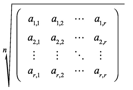
In this study, we consider the finite-dimensional case, so that the general operator under consideration can be represented as a $r\times r$ ($r\in \mathbb{N}$) complex-valued matrix $𝒜$.

We denote as:

$$\left\{\begin{array}{c}{u}_1=tr𝒜=a_{11}+a_{22}+\dots +a_{rr}\hfill \\ {\displaystyle u_2=\sum _{i<j}^{1,r}\left|\begin{array}{cc}{a}_{ii}& a_{ij}\\ a_{ji}& a_{jj}\end{array}\right|}\hfill \\ {\displaystyle u_3=\sum _{i<j<k}^{1,r}\left|\begin{array}{ccc}{a}_{ii}& a_{ij}& a_{ik}\\ a_{ji}& a_{jj}& a_{jk}\\ a_{ki}& a_{kj}& a_{kk}\end{array}\right|}\hfill \\ \cdots \hfill \\ u_r=det𝒜\hfill \end{array}\right.$$

(3)

the invariants of $𝒜$, i.e., the coefficients of the characteristic polynomial:

$$\begin{array}{c}\hfill P\left(\lambda \right)={\lambda }^r-u_1{\lambda }^{r-1}+\cdots +{(-1)}^{r-1}{u}_{r-1}\lambda +{(-1)}^r{u}_r,\end{array}$$

(4)

which are invariants under similarity transformations. Let:

$$\begin{array}{c}\hfill {\lambda }_1,{\lambda }_2,\dots ,{\lambda }_r\end{array}$$

(5)

be the roots of $P\left(\lambda \right)$, i.e., the eigenvalues of $𝒜$.

In [22] (pp. 93–95), the following representation of the resolvent ${\left(\lambda \mathcal{I}-𝒜\right)}^{-1}$ in terms of the invariants of $𝒜$ was proven:

$$\begin{array}{c}\hfill {\displaystyle {(\lambda \mathcal{I}-𝒜)}^{-1}=\frac{1}{P\left(\lambda \right)}\sum _{k=0}^{r-1}\sum _{h=0}^{r-k-1}{(-1)}^h{u}_h{\lambda }^{r-k-h-1}{𝒜}^k.}\end{array}$$

(6)

By using (5) and (6), we can easily derive the representation formula for matrix functions reported in [18].

Theorem 2.

Let $f\left(\lambda \right)$ be a holomorphic function in a domain Δ of the complex plane containing the spectrum of $𝒜$, and denote by $\gamma \subset \Delta$ a simple contour enclosing all the zeros of $P\left(\lambda \right)$. Then, the Dunford–Taylor integral is written as:

$$\begin{array}{c}\hfill \begin{array}{c}{\displaystyle f\left(𝒜\right)=\frac{1}{2\pi \mathrm{i}}\sum _{k=1}^r\left[{\displaystyle {\oint }_{\gamma }\frac{f\left(\lambda \right){\sum }_{h=0}^{k-1}{(-1)}^h{u}_h{\lambda }^{k-h-1}}{P\left(\lambda \right)}d\lambda }\right]{𝒜}^{r-k}.}\end{array}\end{array}$$

(7)

It should be noted that, if $\Delta$ does not contain the origin, a simple choice of $\gamma$ is a circle centered at the origin and having a radius larger than the spectral radius of $𝒜$, which can be determined using Gershgorin’s theorem.

Let us consider now the function $f\left(\lambda \right)={\lambda }^{1/n}$, where n is a fixed integer number. As this function is always holomorphic in the open set $\Delta =(\mathbb{C}-\{0\left\}\right)$, i.e., in the whole plane excluding the origin, the preceding theorem can be re-formulated as follows:

Theorem 3.

If $𝒜$ is a non-singular complex-valued matrix and $\gamma \subset \Delta$ is a simple contour enclosing all the zeros of $P\left(\lambda \right)$, then the $n^{\mathrm{th}}$ roots of $𝒜$ can be represented as:

$${\displaystyle {𝒜}^{1/n}=\sum _{k=1}^r{\xi }_k{𝒜}^{r-k},}$$

(8)

with the general coefficient ${\xi }_k$ given by:

$${\displaystyle {\xi }_k=\frac{1}{2\pi \mathrm{i}}{\oint }_{\gamma }\frac{{\lambda }^{1/n}{\sum }_{h=0}^{k-1}{(-1)}^h{u}_h{\lambda }^{k-h-1}}{P\left(\lambda \right)}d\lambda .}$$

(9)

Recalling Cauchy’s residue theorem [25] and denoting the integrand in (9) as $\Phi =\Phi \left(\lambda \right)$, the contour integral can be evaluated as:

$$\begin{array}{c}\hfill \begin{array}{c}{\displaystyle {\oint }_{\gamma }\frac{{\lambda }^{1/n}{\sum }_{h=0}^{k-1}{(-1)}^h{u}_h{\lambda }^{k-h-1}}{P\left(\lambda \right)}d\lambda =2\pi \mathrm{i}\sum _{\ell =1}^{r}Re{s}_{\Phi }\left({\lambda }_{\ell }\right).}\end{array}\end{array}$$

(10)

Assuming, for simplicity, that the eigenvalues are all simple and, therefore:

$$P\left(\lambda \right)=(\lambda -{\lambda }_1)(\lambda -{\lambda }_2)\cdots (\lambda -{\lambda }_r).$$

we find:

$$\begin{array}{c}\begin{array}{c}{\displaystyle Re{s}_{\Phi }\left({\lambda }_{\ell }\right)=\underset{\lambda \to {\lambda }_{\ell }}{lim}(\lambda -{\lambda }_{\ell })\frac{{\lambda }^{1/n}{\sum }_{h=0}^{k-1}{(-1)}^h{u}_h{\lambda }^{k-h-1}}{P\left(\lambda \right)}=}\\ {\displaystyle \phantom{1pt26pt}=\frac{{\lambda }_{\ell }^{1/n}{\sum }_{h=0}^{k-1}{(-1)}^h{u}_h{\lambda }_{\ell }^{k-h-1}}{({\lambda }_{\ell }-{\lambda }_1)\cdots ({\lambda }_{\ell }-{\lambda }_{\ell -1})({\lambda }_{\ell }-{\lambda }_{\ell +1})\cdots ({\lambda }_{\ell }-{\lambda }_r)},}\end{array}\hfill \end{array}$$

(11)

where we have put, by definition, $(\lambda -{\lambda }_0)=(\lambda -{\lambda }_{r+1}):=1$.

Finally, upon combining (10) and (11), it is trivial to verify that (9) becomes:

$${\displaystyle {\xi }_k=\sum _{\ell =1}^{r}Re{s}_{\Phi }\left({\lambda }_{\ell }\right)=\sum _{\ell =1}^r\frac{{\lambda }_{\ell }^{1/n}{\sum }_{h=0}^{k-1}{(-1)}^h{u}_h{\lambda }_{\ell }^{k-h-1}}{({\lambda }_{\ell }-{\lambda }_1)\cdots ({\lambda }_{\ell }-{\lambda }_{\ell -1})({\lambda }_{\ell }-{\lambda }_{\ell +1})\cdots ({\lambda }_{\ell }-{\lambda }_r)}.}$$

(12)

A similar result can be found in the case of multiple roots of the characteristic polynomial by using the following more general equation, which holds true for a pole of order m at the point ${\lambda }_{\ell }$:

$$\begin{array}{c}\hfill \begin{array}{c}{\displaystyle Re{s}_{\Phi }\left({\lambda }_{\ell }\right)=\frac{1}{(m-1)!}\underset{\lambda \to {\lambda }_{\ell }}{lim}\frac{d^{m-1}}{d{\lambda }^{m-1}}\left[{(\lambda -{\lambda }_{\ell })}^{m}f\left(\lambda \right)\right].}\end{array}\end{array}$$

(13)

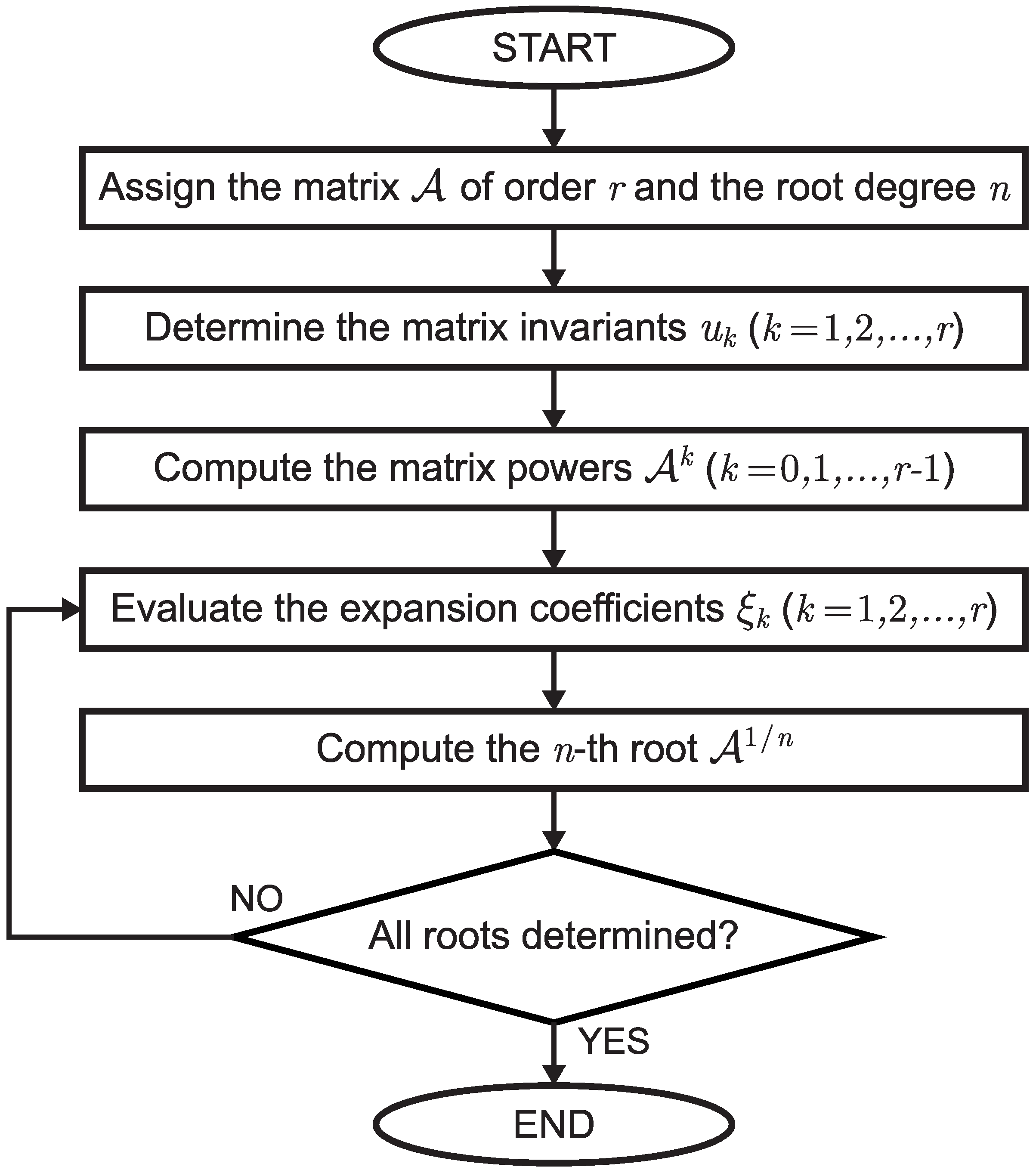
Remark 1.

Note that the knowledge of the eigenvalues is not necessary unless the integral in (7) is computed by means of Cauchy’s residue theorem. In general, only the knowledge of the matrix invariants is sufficient to evaluate the considered contour integral by choosing, as γ, a circle centered at the origin with a radius larger than the spectral radius of $𝒜$. Examples of computations using Cauchy’s residue theorem were given in [16].

Remark 2.

Note that, upon selecting the different determinations of the root function of degree n in the formal expression of ${𝒜}^{1/n}$, it is possible to evaluate the various roots of $𝒜$ through Equation (8).

Based on Theorem 3, the proposed algorithm for the evaluation of the $n^{\mathrm{th}}$ roots of a matrix $𝒜$ can be described through the flowchart illustrated in Figure 1. It is straightforward to verify that the computational complexity of the relevant numerical procedure is $O\left(r^4\right)$ in the worst case.

4. Examples

4.1. Square Root of a $\mathbf{6}\times \mathbf{6}$ Non-Singular Matrix

Consider the matrix:

$$𝒜=\left(\begin{array}{cccccc}\hfill 1& \hfill -2& \hfill 0& \hfill 1& \hfill 3& \hfill 3\\ \hfill 0& \hfill 2& \hfill 0& \hfill 0& \hfill -3& \hfill -2\\ \hfill 8& \hfill 4& \hfill -1& \hfill -2& \hfill 6& \hfill 7\\ \hfill 4& \hfill 1& \hfill -1& \hfill 1& \hfill 2& \hfill 5\\ \hfill -3& \hfill 0& \hfill 0& \hfill 1& \hfill -4& \hfill -3\\ \hfill 2& \hfill 1& \hfill 0& \hfill -1& \hfill 2& \hfill 1\end{array}\right)$$

(14)

The relevant invariants are:

$$u_1=0,u_2=-4,u_3=0,u_4=-1,u_5=0,u_6=4$$

(15)

whereas the corresponding eigenvalues are found to be:

$${\lambda }_1=-2,{\lambda }_2=2,{\lambda }_3=-1,{\lambda }_4=\mathrm{i},{\lambda }_5=-\mathrm{i},{\lambda }_6=1.$$

(16)

Putting:

$${𝒜}^{1/2}=\mathrm{Re}\left\{{𝒜}^{1/2}\right\}+\mathrm{i}\mathrm{Im}\left\{{𝒜}^{1/2}\right\},$$

(17)

we find:

$$Re\left\{{𝒜}^{1/2}\right\}=\left(\begin{array}{cccccc}\frac{1}{60}\left(71\sqrt{2}-10\right)& \frac{1}{60}\left(-30-13\sqrt{2}\right)& \frac{1}{6}\left(\sqrt{2}-1\right)& \frac{1}{3}-\frac{1}{5\sqrt{2}}& \frac{1}{60}\left(20+57\sqrt{2}\right)& \frac{1}{2}+\frac{4\sqrt{2}}{5}\\ \frac{1}{60}\left(35-34\sqrt{2}\right)& \frac{7}{4}+\frac{1}{15\sqrt{2}}& -\frac{7}{12}\left(\sqrt{2}-1\right)& \frac{9}{5\sqrt{2}}-\frac{7}{6}& \frac{1}{60}\left(-70-33\sqrt{2}\right)& \frac{1}{20}\left(11\sqrt{2}-35\right)\\ \frac{1}{60}\left(55+37\sqrt{2}\right)& \frac{1}{60}\left(165-101\sqrt{2}\right)& \frac{1}{60}\left(55-7\sqrt{2}\right)& \frac{11}{30}\left(3\sqrt{2}-5\right)& \frac{1}{30}\left(93\sqrt{2}-55\right)& \frac{1}{20}\left(57\sqrt{2}-55\right)\\ \frac{5}{12}+\frac{4\sqrt{2}}{5}& \frac{5}{4}-\frac{2\sqrt{2}}{5}& \frac{1}{60}\left(25-39\sqrt{2}\right)& \frac{13}{5\sqrt{2}}-\frac{5}{6}& \frac{3}{2\sqrt{2}}-\frac{5}{6}& \frac{1}{20}\left(43\sqrt{2}-25\right)\\ \frac{1}{12}\left(1-9\sqrt{2}\right)& \frac{1}{4}\left(1+\sqrt{2}\right)& \frac{1}{60}\left(5-21\sqrt{2}\right)& \frac{2\sqrt{2}}{5}-\frac{1}{6}& -\frac{1}{6}-\frac{9}{5\sqrt{2}}& \frac{1}{4}\left(-1-\sqrt{2}\right)\\ \frac{1}{6}& \frac{1}{2}-\frac{1}{\sqrt{2}}& \frac{1}{30}\left(5+3\sqrt{2}\right)& \frac{1}{5\sqrt{2}}-\frac{1}{3}& \frac{9}{5\sqrt{2}}-\frac{1}{3}& \frac{1}{\sqrt{2}}-\frac{1}{2}\end{array}\right)$$

(18)

$$\mathrm{Im}\left\{{𝒜}^{1/2}\right\}=\left(\begin{array}{cccccc}\frac{1}{12}\left(5\sqrt{2}-4\right)& \frac{1}{12}\left(3\sqrt{2}-4\right)& \frac{1}{15}\left(5-2\sqrt{2}\right)& -\frac{2\sqrt{2}}{15}& \frac{13}{30\sqrt{2}}& \frac{1}{\sqrt{2}}-1\\ \frac{1}{12}\left(5\sqrt{2}-1\right)& \frac{1}{12}\left(3\sqrt{2}-1\right)& \frac{1}{60}\left(5-8\sqrt{2}\right)& -\frac{2\sqrt{2}}{15}& \frac{13}{30\sqrt{2}}& \frac{1}{\sqrt{2}}-\frac{1}{4}\\ \frac{1}{12}\left(19-50\sqrt{2}\right)& \frac{19}{12}-\frac{5}{\sqrt{2}}& \frac{4\sqrt{2}}{3}-\frac{19}{12}& \frac{4\sqrt{2}}{3}& -\frac{13}{3\sqrt{2}}& \frac{19}{4}-5\sqrt{2}\\ \frac{1}{12}\left(-3-5\sqrt{2}\right)& \frac{1}{4}\left(-1-\sqrt{2}\right)& \frac{1}{4}+\frac{2\sqrt{2}}{15}& \frac{2\sqrt{2}}{15}& -\frac{13}{30\sqrt{2}}& -\frac{3}{4}-\frac{1}{\sqrt{2}}\\ \frac{5\sqrt{2}}{3}-\frac{3}{4}& \sqrt{2}-\frac{3}{4}& \frac{3}{4}-\frac{8\sqrt{2}}{15}& -\frac{8\sqrt{2}}{15}& \frac{13\sqrt{2}}{15}& 2\sqrt{2}-\frac{9}{4}\\ 1-\frac{5\sqrt{2}}{3}& 1-\sqrt{2}& \frac{8\sqrt{2}}{15}-1& \frac{8\sqrt{2}}{15}& -\frac{13\sqrt{2}}{15}& 3-2\sqrt{2}\end{array}\right)$$

(19)

It is not difficult to verify that:

$${\left({𝒜}^{1/2}\right)}^2-𝒜={\mathcal{O}}_6,$$

with ${\mathcal{O}}_6$ denoting the zero matrix of order six.

4.2. Cubic Root of a $\mathbf{5}\times \mathbf{5}$ Non-Singular Matrix

Consider the matrix:

$$𝒜=\left(\begin{array}{ccccc}\hfill -8693722& \hfill 4346843& \hfill -4346851& \hfill 4346851& \hfill -9\\ \hfill 3335561& \hfill -1667774& \hfill 1667777& \hfill -1667776& \hfill 2\\ \hfill 38080793& \hfill -19040315& \hfill 19040350& \hfill -19040347& \hfill 39\\ \hfill 17357336& \hfill -8678630& \hfill 8678646& \hfill -8678645& \hfill 19\\ \hfill 18089316& \hfill -9044623& \hfill 9044638& \hfill -9044636& \hfill 16\end{array}\right)$$

(20)

The relevant invariants are:

$$u_1=225,u_2=15055,u_3=335655,u_4=2048824,u_5=1728000$$

(21)

whereas the corresponding eigenvalues are found to be:

$${\lambda }_1=125,{\lambda }_2=64,{\lambda }_3=27,{\lambda }_4=8,{\lambda }_5=1.$$

(22)

We find:

$${𝒜}^{1/3}=\left(\begin{array}{ccccc}-\frac{550639692034711}{5080863606}& \frac{92292354791999}{1693621202}& -\frac{276892879819117}{5080863606}& \frac{19894689325307}{362918829}& -\frac{30446809252}{2540431803}\\ \frac{35442617545992}{846810601}& -\frac{53470087177853}{2540431803}& \frac{53475165103408}{2540431803}& -\frac{7685586295792}{362918829}& \frac{4154804876}{846810601}\\ \frac{1206517116655057}{2540431803}& -\frac{202223214891122}{846810601}& \frac{86672336394136}{362918829}& -\frac{610286406219277}{2540431803}& \frac{134332737209}{2540431803}\\ \frac{2198065365953581}{10161727212}& -\frac{1105223638927307}{10161727212}& \frac{1105286905814213}{10161727212}& -\frac{277945100292131}{2540431803}& \frac{121949841985}{5080863606}\\ \frac{328104046034725}{1451675316}& -\frac{1154921972562721}{10161727212}& \frac{384994878724441}{3387242404}& -\frac{96822304734112}{846810601}& \frac{133570410865}{5080863606}\end{array}\right)$$

(23)

It is not difficult to verify that:

$${\left({𝒜}^{1/3}\right)}^3-𝒜={\mathcal{O}}_5,$$

with ${\mathcal{O}}_5$ denoting the zero matrix of order five.

4.3. Another Cubic Root of a $\mathbf{5}\times \mathbf{5}$ Non-Singular Matrix

Consider the matrix:

$$𝒜=\left(\begin{array}{ccccc}\hfill 62& \hfill -49& \hfill 41& \hfill -41& \hfill -9\\ \hfill -15& \hfill 14& \hfill -11& \hfill 12& \hfill 2\\ \hfill -243& \hfill 203& \hfill -168& \hfill 171& \hfill 39\\ \hfill -122& \hfill 99& \hfill -83& \hfill 84& \hfill 19\\ \hfill -106& \hfill 88& \hfill -73& \hfill 75& \hfill 16\end{array}\right)$$

(24)

The relevant invariants are:

$$u_1=8,u_2=0,u_3=0,u_4=-1,u_5=-8$$

(25)

whereas the corresponding eigenvalues are found to be:

$${\lambda }_1=8,{\lambda }_2=-1,{\lambda }_3=\mathrm{i},{\lambda }_4=-\mathrm{i},{\lambda }_5=1.$$

(26)

Putting:

$${𝒜}^{1/3}=\mathrm{Re}\left\{{𝒜}^{1/3}\right\}+\mathrm{i}\mathrm{Im}\left\{{𝒜}^{1/3}\right\},$$

(27)

we find:

$$\mathrm{Re}\left\{{𝒜}^{1/3}\right\}=\left(\begin{array}{ccccc}\frac{1}{780}\left(4762+963\sqrt{3}\right)& \frac{1}{910}\left(756\sqrt{3}-14071\right)& \frac{57796-6741\sqrt{3}}{5460}& \frac{1}{546}\left(3591\sqrt{3}-11623\right)& \frac{12799}{2730}-\frac{267\sqrt{3}}{65}\\ \frac{1}{390}\left(-449-96\sqrt{3}\right)& \frac{1}{455}\left(2157+133\sqrt{3}\right)& \frac{672\sqrt{3}-7907}{2730}& \frac{1}{273}\left(1760-483\sqrt{3}\right)& \frac{83\sqrt{3}}{65}-\frac{2453}{1365}\\ -\frac{19}{780}\left(787+213\sqrt{3}\right)& \frac{1}{910}\left(59014-2569\sqrt{3}\right)& \frac{28329\sqrt{3}-238009}{5460}& \frac{50041}{546}-\frac{368\sqrt{3}}{13}& \frac{48951\sqrt{3}-56656}{2730}\\ \frac{-15733-3852\sqrt{3}}{1560}& \frac{56739-2569\sqrt{3}}{1820}& \frac{26964\sqrt{3}-235279}{10920}& \frac{12169}{273}-\frac{697\sqrt{3}}{52}& \frac{46221\sqrt{3}-52561}{5460}\\ \frac{-13157-3468\sqrt{3}}{1560}& \frac{1}{260}\left(7263-313\sqrt{3}\right)& \frac{3468\sqrt{3}-29873}{1560}& \frac{3091}{78}-\frac{631\sqrt{3}}{52}& \frac{1}{780}\left(5997\sqrt{3}-6497\right)\end{array}\right)$$

(28)

$$\mathrm{Im}\left\{{𝒜}^{1/3}\right\}=\left(\begin{array}{ccccc}-\frac{47}{12\sqrt{3}}& 0& -\frac{47}{12\sqrt{3}}& -\frac{47}{6\sqrt{3}}& \frac{47}{3\sqrt{3}}\\ \frac{7}{6\sqrt{3}}& 0& \frac{7}{6\sqrt{3}}& \frac{7}{3\sqrt{3}}& -\frac{14}{3\sqrt{3}}\\ \frac{103}{6\sqrt{3}}& 0& \frac{103}{6\sqrt{3}}& \frac{103}{3\sqrt{3}}& -\frac{206}{3\sqrt{3}}\\ \frac{197}{24\sqrt{3}}& 0& \frac{197}{24\sqrt{3}}& \frac{197}{12\sqrt{3}}& -\frac{197}{6\sqrt{3}}\\ \frac{169}{24\sqrt{3}}& 0& \frac{169}{24\sqrt{3}}& \frac{169}{12\sqrt{3}}& -\frac{169}{6\sqrt{3}}\end{array}\right)$$

(29)

It is not difficult to verify that:

$${\left({𝒜}^{1/3}\right)}^3-𝒜={\mathcal{O}}_5,$$

with ${\mathcal{O}}_5$ denoting, as usual, the zero matrix of order five.

4.4. Fifth Root of a $\mathbf{4}\times \mathbf{4}$ Non-Singular Matrix

Consider the matrix:

$$𝒜=\left(\begin{array}{cccc}\hfill -4& \hfill 291& \hfill 285& \hfill -294\\ \hfill -1& \hfill 65& \hfill 63& \hfill -65\\ \hfill 1& \hfill -127& \hfill -126& \hfill 129\\ \hfill 1& \hfill -98& \hfill -97& \hfill 99\end{array}\right)$$

(30)

The relevant invariants are:

$$u_1=34,u_2=63,u_3=-34,u_4=-64$$

(31)

whereas the corresponding eigenvalues are found to be:

$${\lambda }_1=32,{\lambda }_2=2,{\lambda }_3=-1,{\lambda }_5=1.$$

(32)

Putting:

$${𝒜}^{1/5}=\mathrm{Re}\left\{{𝒜}^{1/5}\right\}+\mathrm{i}\mathrm{Im}\left\{{𝒜}^{1/5}\right\},$$

(33)

we find:

$$\mathrm{Re}\left\{{𝒜}^{1/5}\right\}=\left(\begin{array}{cccc}-\frac{50379}{13640}+\frac{43}{52^{4/5}}+\frac{3\sqrt{5}}{88}& \frac{492579}{13640}-\frac{129\sqrt[5]{2}}{5}-\frac{3\sqrt{5}}{88}& \frac{305757}{13640}-\frac{129}{52^{4/5}}+\frac{3\sqrt{5}}{88}& \frac{3\left(-104089+58652\sqrt[5]{2}+155\sqrt{5}\right)}{13640}\\ -\frac{7871}{6820}+\frac{16\sqrt[5]{2}}{15}+\frac{\sqrt{5}}{132}& \frac{198293}{20460}-\frac{32\sqrt[5]{2}}{5}-\frac{\sqrt{5}}{132}& \frac{108739}{20460}-\frac{16\sqrt[5]{2}}{5}+\frac{\sqrt{5}}{132}& -\frac{110909}{20460}+\frac{16\sqrt[5]{2}}{5}+\frac{\sqrt{5}}{132}\\ \frac{79107-87296\sqrt[5]{2}+4495\sqrt{5}}{40920}& -\frac{695987}{40920}+\frac{64\sqrt[5]{2}}{5}-\frac{29\sqrt{5}}{264}& -\frac{409381}{40920}+\frac{32\sqrt[5]{2}}{5}+\frac{29\sqrt{5}}{264}& \frac{428291}{40920}-\frac{32\sqrt[5]{2}}{5}+\frac{29\sqrt{5}}{264}\\ \frac{5839-7502\sqrt[5]{2}+775\sqrt{5}}{6820}& -\frac{65899}{6820}+\frac{33\sqrt[5]{2}}{5}-\frac{5\sqrt{5}}{44}& -\frac{46697}{6820}+\frac{33}{52^{4/5}}+\frac{5\sqrt{5}}{44}& \frac{49487}{6820}-\frac{33}{52^{4/5}}+\frac{5\sqrt{5}}{44}\end{array}\right)$$

(34)

$$\mathrm{Im}\left\{{𝒜}^{1/5}\right\}=\left(\begin{array}{cccc}\frac{3}{22}\sqrt{\frac{5}{8}-\frac{\sqrt{5}}{8}}& -\frac{3}{22}\sqrt{\frac{5}{8}-\frac{\sqrt{5}}{8}}& \frac{3}{22}\sqrt{\frac{5}{8}-\frac{\sqrt{5}}{8}}& \frac{3}{22}\sqrt{\frac{5}{8}-\frac{\sqrt{5}}{8}}\\ \frac{1}{33}\sqrt{\frac{5}{8}-\frac{\sqrt{5}}{8}}& -\frac{1}{33}\sqrt{\frac{5}{8}-\frac{\sqrt{5}}{8}}& \frac{1}{33}\sqrt{\frac{5}{8}-\frac{\sqrt{5}}{8}}& \frac{1}{33}\sqrt{\frac{5}{8}-\frac{\sqrt{5}}{8}}\\ \frac{29}{66}\sqrt{\frac{5}{8}-\frac{\sqrt{5}}{8}}& -\frac{29}{66}\sqrt{\frac{5}{8}-\frac{\sqrt{5}}{8}}& \frac{29}{66}\sqrt{\frac{5}{8}-\frac{\sqrt{5}}{8}}& \frac{29}{66}\sqrt{\frac{5}{8}-\frac{\sqrt{5}}{8}}\\ \frac{5}{11}\sqrt{\frac{5}{8}-\frac{\sqrt{5}}{8}}& -\frac{5}{11}\sqrt{\frac{5}{8}-\frac{\sqrt{5}}{8}}& \frac{5}{11}\sqrt{\frac{5}{8}-\frac{\sqrt{5}}{8}}& \frac{5}{11}\sqrt{\frac{5}{8}-\frac{\sqrt{5}}{8}}\end{array}\right)$$

(35)

It is not difficult to verify that:

$${\left({𝒜}^{1/5}\right)}^5-𝒜={\mathcal{O}}_4,$$

with ${\mathcal{O}}_4$ denoting the zero matrix of order four.

4.5. Square Root of a $\mathbf{3}\times \mathbf{3}$ Non-Singular Matrix

Consider the complex-valued matrix:

$$𝒜=\left(\begin{array}{ccc}1& 0& 0\\ 5& \mathrm{i}& -2-\mathrm{i}\\ 3& 0& -1\end{array}\right)$$

(36)

The relevant invariants are:

$$u_1=\mathrm{i},u_2=-1,u_3=-\mathrm{i}$$

(37)

whereas the corresponding eigenvalues are found to be:

$${\lambda }_1=-1,{\lambda }_2=\mathrm{i},{\lambda }_3=1.$$

(38)

By taking the various determinations of the square root function, we find:

$${𝒜}^{1/2}=\left(\begin{array}{ccc}1& 0& 0\\ \left(\frac{3}{4}-\frac{\mathrm{i}}{4}\right)\left(\sqrt{2}+2-2\mathrm{i}\right)& \frac{1+\mathrm{i}}{\sqrt{2}}& \left(-1-\frac{\mathrm{i}}{2}\right)\left(\sqrt{2}-1-\mathrm{i}\right)\\ \frac{3}{2}-\frac{3\mathrm{i}}{2}& 0& \mathrm{i}\end{array}\right)$$

(39)

$${𝒜}^{1/2}=\left(\begin{array}{ccc}-1& 0& 0\\ \left(\frac{3}{4}-\frac{\mathrm{i}}{4}\right)\left(\sqrt{2}-2-4\mathrm{i}\right)& \frac{1+\mathrm{i}}{\sqrt{2}}& \left(-1-\frac{\mathrm{i}}{2}\right)\left(\sqrt{2}-1-\mathrm{i}\right)\\ -\frac{3}{2}-\frac{3\mathrm{i}}{2}& 0& \mathrm{i}\end{array}\right)$$

(40)

$${𝒜}^{1/2}=\left(\begin{array}{ccc}1& 0& 0\\ \left(-\frac{3}{4}+\frac{\mathrm{i}}{4}\right)\left(\sqrt{2}-2+2\mathrm{i}\right)& -\frac{1+\mathrm{i}}{\sqrt{2}}& \left(1+\frac{\mathrm{i}}{2}\right)\left(\sqrt{2}+1+\mathrm{i}\right)\\ \frac{3}{2}-\frac{3\mathrm{i}}{2}& 0& \mathrm{i}\end{array}\right)$$

(41)

$${𝒜}^{1/2}=\left(\begin{array}{ccc}-1& 0& 0\\ \left(-\frac{3}{4}+\frac{\mathrm{i}}{4}\right)\left(\sqrt{2}+2+4\mathrm{i}\right)& -\frac{1+\mathrm{i}}{\sqrt{2}}& \left(1+\frac{\mathrm{i}}{2}\right)\left(\sqrt{2}+1+\mathrm{i}\right)\\ -\frac{3}{2}-\frac{3\mathrm{i}}{2}& 0& \mathrm{i}\end{array}\right)$$

(42)

$${𝒜}^{1/2}=\left(\begin{array}{ccc}1& 0& 0\\ \left(\frac{3}{4}-\frac{\mathrm{i}}{4}\right)\left(\sqrt{2}+2+4\mathrm{i}\right)& \frac{1+\mathrm{i}}{\sqrt{2}}& \left(-1-\frac{\mathrm{i}}{2}\right)\left(\sqrt{2}+1+\mathrm{i}\right)\\ \frac{3}{2}+\frac{3\mathrm{i}}{2}& 0& -\mathrm{i}\end{array}\right)$$

(43)

$${𝒜}^{1/2}=\left(\begin{array}{ccc}-1& 0& 0\\ \frac{1}{2}\left(-2+4\mathrm{i}+\sqrt{4-3\mathrm{i}}\right)& \frac{1+\mathrm{i}}{\sqrt{2}}& \left(-1-\frac{\mathrm{i}}{2}\right)\left(\sqrt{2}+1+\mathrm{i}\right)\\ -\frac{3}{2}+\frac{3\mathrm{i}}{2}& 0& -\mathrm{i}\end{array}\right)$$

(44)

$${𝒜}^{1/2}=\left(\begin{array}{ccc}1& 0& 0\\ \left(-\frac{3}{4}+\frac{\mathrm{i}}{4}\right)\left(\sqrt{2}-2-4\mathrm{i}\right)& -\frac{1+\mathrm{i}}{\sqrt{2}}& \left(1+\frac{\mathrm{i}}{2}\right)\left(\sqrt{2}-1-\mathrm{i}\right)\\ \frac{3}{2}+\frac{3\mathrm{i}}{2}& 0& -\mathrm{i}\end{array}\right)$$

(45)

$${𝒜}^{1/2}=\left(\begin{array}{ccc}-1& 0& 0\\ -1+2\mathrm{i}-\frac{1}{2}\sqrt{4-3\mathrm{i}}& -\frac{1+\mathrm{i}}{\sqrt{2}}& \left(1+\frac{\mathrm{i}}{2}\right)\left(\sqrt{2}-1-\mathrm{i}\right)\\ -\frac{3}{2}+\frac{3\mathrm{i}}{2}& 0& -\mathrm{i}\end{array}\right)$$

(46)

For each one of the $n^r=8$ roots, it is not difficult to verify that:

$${\left({𝒜}^{1/2}\right)}^2-𝒜={\mathcal{O}}_3,$$

with ${\mathcal{O}}_3$ denoting the zero matrix of order three.

5. Conclusions

A general method for computing the $n^{\mathrm{th}}$ roots of complex-valued matrices was detailed. The proposed procedure was based on the application of the Dunford–Taylor integral in combination with a suitable representation formula of the matrix resolvent. In this way, it was possible to overcome the limitations of the techniques already available in the scientific literature, in terms of the matrix order, as well as of the root degree.

The presented approach provided an effective means for evaluating all the determinations of the root of a given matrix with a reduced computational complexity and burden since it relied, only, on the knowledge of the matrix invariants, so circumventing the need for computing the relevant eigenvalues, while the spectral radius could be estimated using Gershgorin’s theorem. Several worked examples were provided to prove the correctness of the procedure for higher order real- and complex-valued matrices.

References

1. Gantmacher, F.R. The Theory of Matrices; Chelsea Pub. Co.: New York, NY, USA, 1959. [Google Scholar]
2. Levinger, B.W. The square root of a 2 × 2 matrix. Math. Mag. 1980, 53, 222–224. [Google Scholar] [CrossRef]
3. Sullivan, D. The square roots of 2 × 2 matrices. Math. Mag. 1993, 66, 314–316. [Google Scholar] [CrossRef]
4. Yood, B. Rootless matrices. Math. Mag. 2002, 75, 219–223. [Google Scholar] [CrossRef]
5. Choudhry, A. Extraction of nth roots of 2 × 2 matrices. Linear Algebra Appl. 2004, 387, 183–192. [Google Scholar] [CrossRef] [Green Version]
6. Johnson, C.R.; Okubo, K.; Reams, R. Uniqueness of matrix square roots and an application. Linear Algebra Appl. 2001, 323, 51–60. [Google Scholar] [CrossRef] [Green Version]
7. Higham, N. Functions of Matrices. Theory and Computation; SIAM: Philadelphia, PA, USA, 2008. [Google Scholar]
8. Al-Tamimi, I.A. The square roots of 2 × 2 invertible matrices. Adv. Algebra 2010, 3, 15–18. [Google Scholar]
9. Rao, S.S.; Jagadeeshwar, P.; Somasekhar, K. On the square root of a matrix. JGRMA 2013, 1, 30–33. [Google Scholar]
10. Psarrakos, P.J. On the mth roots of a complex matrix. Electron. J. Linear Algebra 2002, 9, 32–41. [Google Scholar] [CrossRef] [Green Version]
11. Ricci, P.E.; Srivastava, R. A study of the second-kind multivariate pseudo-Chebyshev functions of fractional degree. Mathematics 2020. submitted. [Google Scholar]
12. Ricci, P.E. Alcune osservazioni sulle potenze delle matrici del secondo ordine e sui polinomi di Tchebycheff di seconda specie. Atti Accad. Sci. Torino 1975, 109, 405–410. [Google Scholar]
13. Ricci, P.E. Sulle potenze di una matrice. Rend. Mat. 1976, 9, 179–194. [Google Scholar]
14. Ricci, P.E. Complex spirals and pseudo-Chebyshev polynomials of fractional degree. Symmetry 2018, 10, 671. [Google Scholar] [CrossRef] [Green Version]
15. Ricci, P.E. A survey on pseudo-Chebyshev functions. 4Open 2019. submitted. [Google Scholar]
16. Ricci, P.E. On the roots of complex r × r matrices. Lect. Notes TICMI 2020. to appear. [Google Scholar]
17. Lucas, É. Théorie des Nombres; Gauthier-Villars: Paris, France, 1891. [Google Scholar]
18. Bruschi, M.; Ricci, P.E. An explicit formula for f(𝒜) and the generating function of the generalized Lucas polynomials. Siam J. Math. Anal. 1982, 13, 162–165. [Google Scholar] [CrossRef]
19. Natalini, P.; Ricci, P.E. A “hard to die” series expansion and Lucas polynomials of the second kind. Appl. Math. 2015, 6, 1235–1240. [Google Scholar] [CrossRef] [Green Version]
20. Natalini, P.; Ricci, P.E. Solution of linear dynamical systems using Lucas polynomials of the second kind. Appl. Math. 2016, 7, 616–628. [Google Scholar] [CrossRef] [Green Version]
21. Mitchell, D.W. Using Pythagorean triples to generate square roots of I2. Math. Gaz. 2003, 87, 499–500. [Google Scholar] [CrossRef]
22. Cherubino, S. Calcolo delle Matrici; Cremonese: Rome, Italy, 1957. [Google Scholar]
23. Kato, T. Perturbation Theory for Linear Operators; Springer: Berlin/Heidelberg, Germany, 1966. [Google Scholar]
24. Bruschi, M.; Ricci, P.E. Sulle funzioni Fk,n e i polinomi di Lucas di seconda specie generalizzati. Pubbl. Ist. Mat. Appl. Fac. Ing. Univ. Stud. Roma 1979, 14, 49–58. [Google Scholar]
25. Rudin, W. Real and Complex Analysis, 3rd ed.; McGraw-Hill: Singapore, 1987. [Google Scholar]
Figure 1. Flowchart of the algorithm for the evaluation of the n th roots of a given matrix 𝒜 .
Symmetry 12 00966 g001