On Path Homology of Vertex Colored (Di)Graphs


Faculty of Mathematics and Computer Science, University of Warmia and Mazury in Olsztyn, Słoneczna 54, 10-710 Olsztyn, Poland
*
Author to whom correspondence should be addressed.
Symmetry 2020, 12(6), 965; https://doi.org/10.3390/sym12060965
Submission received: 6 May 2020
/
Revised: 31 May 2020
/
Accepted: 1 June 2020
/
Published: 5 June 2020
Abstract
:In this paper, we construct the colored-path homology theory in the category of vertex colored (di)graphs and describe its basic properties. Our construction is based on the path homology theory of digraphs that was introduced in the papers of Grigoryan, Muranov, and Shing-Tung Yau and stems from the notion of the path complex. Any graph naturally gives rise to a path complex in which for a given set of vertices, paths go along the edges of the graph. We define path complexes of vertex colored (di)graphs using the natural restrictions that are given by coloring. Thus, we obtain a new collection of colored-path homology theories. We introduce the notion of colored homotopy and prove functoriality as well as homotopy invariance of homology groups. For any colored digraph, we construct the spectral sequence of colored-path homology groups which gives the effective method of computations in the general case since any (di)graph can be equipped with various colorings. We provide a lot of examples to illustrate our results as well as methods of computations. We introduce the notion of homotopy and prove functoriality and homotopy invariance of introduced vertexed colored-path homology groups. For any colored digraph, we construct the spectral sequence of path homology groups which gives the effective method of computations in the constructed theory. We provide a lot of examples to illustrate obtained results as well as methods of computations.
1. Introduction
In this paper, we apply the methods of the path homology theory of digraphs and quivers first defined in [1,2,3,4,5,6] to the category and homotopy category of vertex colored digraphs and graphs (see [7,8,9,10,11]).
We construct the collection of path homology theories for vertex colored digraphs. Then we describe the possibility of implementing this theory to the case of edge colored digraphs and non-directed graphs. We will consider vertex colored (di)graphs which from now on will be simply called colored (di)graphs unless otherwise clearly stated.
The consideration of digraphs in this theory stems from the following reasons. The path homology theory is a natural generalization of simplicial homology theory and is defined for any path complex. Any digraph naturally gives rise to a path complex in which allowed paths go along directed edges. The path homology theory for digraphs provides the path homology theory for (non-directed) graphs by applying the functorial transformation from a given graph to the corresponding symmetric digraph [2].
In the classical algebraic topology, in most cases, the homology groups have a natural filtration that is given by the n-skeleton of or a simplicial complex. In the general case, the path homology groups do not have any structure that is similar to the n-skeleton. It follows directly from the results below that a vertex coloring of a digraph gives a functorial filtration that agrees with path homology groups. If we color a digraph in some way, then by the means of the spectral sequence constructed below, we obtain an effective method of computing the path homology groups of such a (di)graph.
Note also that the line digraph of an edge colored digraph gives the vertex colored digraph and that means in turn that the vertex colored homology theory might be applied to the edge colored digraphs and non-directed graphs. Let us mention here that the application of the colored homology theory to the case of quivers requires significant modifications. This fact follows from the generalization of the path homology theory to the category of quivers constructed in [4].
In our paper, we use the notions of the category and the functor (see, for example, ([10,12], Chapter 1) and ([13], Chapter 1)). A category consists of a class of objects and for each ordered pair of objects a collection of morphisms. Any such morphism will be denoted by . For every pair of morphisms , , we define a composition . The morphisms satisfy the following axioms.
- (i)
- If , and , then .
- (ii)
- For every object B there is a morphism , such that if , then and if , then .
Let and be two categories. A functor from to assigns to any object of an object and to any morphism of a morphism in such a way that
- (i)
- ,
- (ii)
- for , .
It is necessary to remark that the notion of homotopy in the graph theory differs from a similar notion in the continuous topology (see Definition 4 and Example 1 below). Two digraph mappings are homotopic if we can construct a sequence of digraph mappings from G to H, so that any pair of sequential mappings satisfies one of the following properties (see ([2], §3.1)):
- (i)
- or in the digraph H for arbitrary vertex v of the digraph G,
- (ii)
- or in the digraph H for arbitrary vertex v of the digraph G.
Let us point out here the main new results provided in our paper. First, we introduce the category of colored digraphs and define a notion of the colored homotopy between colored morphisms. Then we describe the basic properties of the colored homotopy and colored morphisms and construct a collection of functorial path homology theories for colored digraphs. We prove the invariance of the colored-path homology groups relative to the colored homotopy. For any colored digraph we construct the spectral sequence of colored-path homology groups which gives the effective method of computations of path homology groups of arbitrary digraphs since any (di)graph can be equipped with various colorings. We also describe the transfer of the colored-path homology theory to the category of graphs and edge colored (di)graphs.
The paper is organized as follows. In Section 2, for the sake of convenience, we recall the basic definitions from the graph theory and the path homology theory for digraphs.
In Section 3, we bring the notion of colored digraphs to your attention and introduce the notion of homotopy for colored digraphs.
In Section 4, we define several path homology theories for the categories that were introduced in the previous Section. Next, we provide examples to illustrate the difference between the path homology theory of digraphs in colored and uncolored case.
In Section 5, we construct a spectral sequence for path homology groups of a colored digraph, and describe its basic properties. We also obtain a braid of exact sequences of path homology groups for 3-colored digraphs. We give detailed computations of path homology groups in such a braid of exact sequences for a digraph G that is the one-dimensional skeleton of the minimal triangulation of the closed Möbius band.
In Section 6, we describe applications of the obtained results to the case of non-directed graphs. We also explain the possibility of applying homology of vertex colored digraph to the edge colored digraphs and edge colored graphs using the line digraphs.
Finally, in Section 7, we give conclusions and make some remarks about our results, whereas is acknowledgement section.
2. The Path Homology Theory for Digraphs
In this Section, we give preliminary material about the path homology theory for a digraph following [1,2,3,4,5,6].
Definition 1.
A digraph G is a pair of a set of vertices and a subset of ordered pairs of vertices which are called arrows. A pair is denoted . For such a pair the vertex v is called an origin of the arrow and is denoted while the vertex w is called an end of the arrow and is denoted .
Definition 2.
A digraph mapping (or simply a mapping) from a digraph G to a digraph H is a mapping such that for any arrow , we have or . We call the mapping f non-degenerate if for any . For a digraph G we denote by the identity mapping that is the identity mapping on the set of vertices and the set of edges.
It is clear that digraphs with the digraph mappings form a category which throughout this paper will be denoted by . Please note that digraphs together with non-degenerated mappings form a subcategory of the category .
Definition 3.
For two digraphs and their Box product is a digraph with a set of vertices and a set of arrows given in the following way. For two vertices , and two vertices there is an arrow if and only if
In Example 1 below we give a graph interpretation of the Box product.
Fix . Denote by a digraph for which and, for , there is exactly one arrow or without any other available arrows. We will refer from now on to as a segment digraph. Let us note here that the notion of a segment digraph coincides with the notion of a line digraph introduced in papers [1,2,3,4,5,6]. We are forced to use different terminology because the standard notion of a line digraph already exists in the graph theory and will also be used later in this paper.
Definition 4.
Two digraph mappings are called homotopic if there exists a segment digraph and a digraph mapping called a homotopy between and , such that
In such a case we write .
Example 1.
Now we give several digraphs to illustrate definitions introduced above.
- (i)
- For the digraph presented on the diagram belowwe have , whereas .
- (ii)
- Let G be a digraph given in (1) and be a digraph provided belowLet be the mapping given by . Then the mapping f is the digraph mapping but it is not a non-degenerate digraph mapping since is not an arrow. Let be the mapping given by . Then the mapping g is the non-degenerate digraph mapping.
- (iii)
- The explanation of the Box product is given in the diagram below:where and .
- (iv)
- Let be the digraph presented on the diagramand be the line digraph . Let be the mapping given on the set of vertices and be the mapping given on the set of vertices . Let I be the segment digraph . Now we define the homotopy between f and g as follows:
In the Figure 1 given below we point out the images of the vertices of the digraph under the homotopy mapping F.
The relation ≃ is an equivalence relation on the set of digraph mappings from G to H. Two digraphs G and H are homotopy equivalent if there exist digraph mappings and such that and , where and are the identity mappings of H and G respectively. In this case, we write and call the mappings f and g homotopy inverses to each other.
Thus, the category with the same objects as in and with the morphisms given by classes of homotopy equivalent digraphs mappings is defined.
A homotopy F is non-degenerate if it is non-degenerate as a digraph mapping. We define a category with the same objects as in and with the morphisms that are given by classes of homotopies by means of the non-degenerate homotopy of non-degenerate mappings.
Now we define the path homology groups of a digraph . For , we define an elementary p-path on a set V as a sequence of of vertices (not necessarily different) and denote this path . Let R be a commutative ring with a unity and let be a free R-module generated by all elementary p-paths . The elements of are called p-paths. Set and for , define the boundary operator on basic elements by
where means omitting the corresponding index. We assume that is trivial. It is easy to check that for any elementary p-path v, we have , hence the homomorphism is trivial for . Let . An elementary p-path is called regular if for . Any 0-path is regular. For , we denote by a submodule of that is generated by all irregular elementary paths. In particular, and we set . It is easy to check that for . Thus, we obtain a chain complex
where and the differential is induced by ∂.
We note here that thus obtained path complex is defined for arbitrary discrete set V but basic elements depend on the order of the vertices in the recording . For example, for the elements and are different. The differential ∂ is well defined for basic elements and, for example .
Now we consider a digraph . Let be a regular elementary p-path on the set of vertices V. For , it is called allowed if for any , and non-allowed otherwise. For any elementary path is regular. For , denote by a submodule of that is generated by the allowed elementary p-paths and set . The elements of the modules are called allowed p-paths.
Now we define the path homologies of a digraph . Consider the following submodule of , namely
The elements of are called ∂-invariant p-paths. Examine now the chain complex
Its homologies are called path homologies of the digraph G with the coefficients in the ring R and are denoted by
Every elementary allowed path of the chain complex (6) has a naturally ordered structure on the set of vertices that is defined by arrows of the digraph. By definition, each pair of neighboring vertices in must give an arrow . The differential ∂ in the chain complex is well defined and preserves this ordering.
The path homology groups give a collection of (di)graphs invariants and provide deep connections of the graph theory to discrete geometry, algebraic topology, and mathematical physics (see, for example [1,6,14,15,16,17]). For the sake of convenience, we formulate the basic result of the categorical properties of path homology groups which will be used throughout this paper.
Theorem 1
([1]). The homology groups defined above are homotopy invariant and functorial for digraph mappings.
3. Categories of Colored Digraphs
In the first part of this section we recall the basic definitions concerning digraph coloring (see [7,8,9,10,11]). Then we describe several categories of colored digraphs that fit the path homology theory defined in Section 2.
Definition 5.
A coloring of a digraph is given by an assignment of a color to each vertex . A coloring that uses k colors is called k-coloring.
Recall that two vertices are called neighbors if there exists at least one arrow or in G. The open neighborhood of a vertex is a subgraph of G, for which consists of all vertices which are neighbors of v while is constituted by the edges connecting vertices from . A coloring of a digraph G is called proper if any vertex of the neighborhood is colored differently from the vertex v for all . A coloring of a digraph G is called k-improper if the open neighborhood of any vertex v contains at most k-vertices with the same color as v. As usual, we can consider a coloring as a function . In the case of k-coloring, we assume that . We shall write for a digraph G with a coloring function .
Definition 6.
Let and be two colored digraphs. A digraph mapping is a morphism of colored digraphs if for any vertex .
It is clear that colored digraphs with the morphisms defined above form a category which from now on will be denoted by . This category has the naturally defined subcategory , objects of which are given by proper colored digraphs and morphisms are given by non-degenerate mappings that satisfy Definition 6. Moreover, if we let be the subcategory of with the objects that are given by k-improper colored digraphs and with morphisms that are given by digraph mappings that satisfy Definition 6, then we obtain a filtration
of the category C. In what follows, we will consider a proper coloring as the k-improper coloring with .
For a colored digraph , we can consider only the digraph G that now is recognized as one without any coloring. Any morphism of colored digraphs is, in particular, a digraph mapping . Thus, we obtain a forgetful functor from the category of colored digraphs to the category of digraphs.
For any colored digraph and a segment digraph , we define a coloring on the digraph by
For a k-improper colored digraph , the coloring gives a -improper coloring of the digraph . We shall say that two morphisms of colored digraphs are colored homotopic if there exists a homotopy in Definition 4 such that
We will denote this relation exactly as before, namely ≃, since the category under investigation will be clear from the given context.
Proposition 1.
The relation “to be colored homotopic” is an equivalence relation on the set of colored morphisms and provides a relation ≃ of colored homotopy equivalence of colored digraphs.
Proof.
Consider the set of colored morphisms . Since is the one-vertex digraph we obtain and the colored morphism gives . The proof of the remaining properties follows from corresponding results for digraph mappings.
Thus, we obtain the colored homotopy category in which the objects are colored digraphs and morphisms are classes of colored homotopic morphisms.
Proposition 2.
(i) Any morphism of proper colored digraphs is non-degenerate. (ii) Two morphisms of proper colored digraphs are colored homotopic if and only if .
Proof.
The statement (i) is known and results directly from Definitions 2 and 6. To prove (ii), we must check only that the colored homotopic mappings coincide. Consider the case and let be a colored homotopy. For any vertex , due to the definition we have an arrow and . If , then we are provided with an arrow in . This is impossible in a proper colored digraph H since, by (9), . Thus, for any vertex . Performing induction by n and using the same line of arguments finishes the proof. □
Now we give several examples that explain that the introduced notions are non-degenerate.
Example 2.
- (i)
- Let G be the 1-improper colored digraph presented on (10).Let be the identity mapping and be the mapping defined on the set of vertices in the following way . Observe that thus defined, and are colored morphisms. Define the colored homotopy on the set of vertices byThen it follows that is colored homotopic to .
- (ii)
- Let G be the proper colored digraph presented on (11):By Proposition 2, any two different colored morphisms are not colored homotopic. By ([2], Ex. 3.12) digraph G is contractible and, hence, any two digraph mappings to G are homotopic. It is a relatively easy exercise to construct directly a homotopy between the identity mapping and the mapping that is given on the set of vertices by
- (iii)
- Using the same line of arguments as in the case (ii) and the results from [2] (Section 3) it is possible to construct a lot of similar examples.
4. Path Homology of Colored Digraphs
Now we turn our attention to defining several path homology theories for colored digraphs and describe relations between them. We will provide examples that illustrate the difference between the path homology theory of digraphs in cases of colored and uncolored ones.
Let be a colored digraph with a given coloring . Fix a natural number .
Definition 7.
An elementary path on the set V of vertices is calledk-colored if vertices of this path are colored with k-colors.
Example 3.
Consider the colored digraph in Figure 2. The path is 2-colored while the path is 3-colored. Please note that any regular elementary p-paths are k-colored where .
For , let be a free R-module generated by all allowed regular elementary p-paths, which are colored by s colors, . Let . We have the following natural inclusions of the modules
Now we define k-colored-path homologies of the colored digraph . Let
be a submodule of . The elements of are called ∂-invariant k-colored paths. Similarly, to the case of path homology, we obtain that . As a result, we have the following chain complex
with the differential that is induced from the differential in . Homology groups of the chain complex (14) are called k-colored path homology groups of a digraph and are denoted by .
Proposition 3.
For any colored digraph , we have a filtration
Moreover, for a k-colored digraph this filtration is finite and .
Proof.
We have natural inclusions and the result arises from (13). □
Example 4.
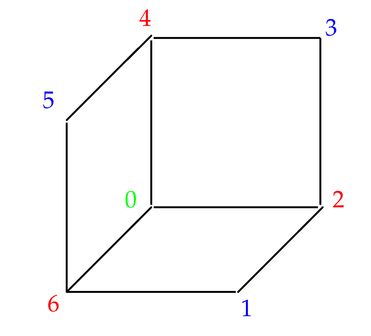
Consider the proper colored digraph cube in Figure 2 with the set of vertices . To simplify computations, we assume that . It arises from [2] that and for .
The module is generated by elements , where and, hence . The modules are trivial since G is proper colored. It follows that
The module is isomorphic to and the module is generated by all arrows. The module is generated by the elements
The module is generated by the elements and , since . The modules are trivial for because there are no paths of the length greater than 3 in G. For more clarity, let us write all the considerations above in the more approachable form, namely
Calculating directly, we provide the following result
Recall that by ([2], 2.5, and Th. 2.10), any digraph mapping defines a morphism of chain complexes
which on the basic elements of the module is given by
Theorem 2.
Let be a morphism of colored digraphs. For , the morphism in (16) provides a morphism of chain complexes
and, hence, an induced homomorphism of k-colored homology groups
Proof.
Now we prove the colored homotopy invariance of colored homology groups of digraphs.
Theorem 3.
Let be two colored homotopic digraph morphisms. Then and induce the identical homomorphisms
of colored homology groups for .
Proof.
It is sufficient to prove the statement for a homotopy in the case . The general case follows by induction.
By Theorem 2, the colored morphisms and F induce morphisms of chain complexes
Please note that we can identify colored digraphs and with the colored digraph G in a natural way. We will denote vertices by i and vertices by . Similar notations will be used for arrows and paths. By the definition of the colored homotopy, for any colored path , we have , while for any colored path , we have . For , define R-linear mappings
on elementary paths in the following way
Corollary 1.
If the colored digraphs and are colored homotopy equivalent, then the colored homology groups and are isomorphic for and mutually inverse isomorphisms of these groups are induced by the homotopy inverse colored morphisms.
Corollary 2.
For , the colored homology groups provide a functor from the colored homotopy category to the category R-modules and homomorphisms.
5. Spectral Sequence for Path Homology Groups of a Colored Digraph
In this section, we construct a spectral sequence for path homology groups of any colored digraph. Our construction is based on the concept of an exact couple of a filtered chain complex from ([18], Chapter 7).
Let be a vertex colored digraph. By Proposition 3 we have a filtration (15) of the chain complex . Let . We define a filtration of by subcomplexes for in the following way
Thus, we have an infinite filtration
Theorem 4.
The filtration (22) has the following properties.
- 1.
- for .
- 2.
- There is a short exact sequence of chain complexeswith for .
- 3.
Proof.
The first statement follows from the definition (21). The elements of the module are given by linear combinations of allowed paths which are colored exactly by colors. Any elementary allowed path can be colored at most by colors. Hence, for (that is for ) the module is trivial. Now we have for and the second statement follows. Any path has a finite number of vertices and is colored by a finite number of colors, thus the third statement is proved. □
Corollary 3.
The exact sequence (23) induces a homology long exact sequence
Now we describe the spectral sequence of the filtration (22) following [18] (Chapter 7). Let
and , be corresponding bigraded R-modules. Consider the homomorphisms of homology groups that follow from exact sequences of the Corollary 3 for various p and :
The homomorphisms in (25) define bigraded homomorphisms
of bidegree , , and respectively.
Proposition 4.
The bigraded modules , and the homomorphisms fit into the commutative diagram
which is exact in each vertex. Thus, we have an exact couple of modules in the sense of [18].
Proof.
The proof in the general case of a chain complex with filtration is given in ([18], Chapter 7). □
Corollary 4.
The exact couple in (27) defines a spectral sequence with the first differential where is given by
of bidegree . The group is isomorphic to the quotient group
The differential coincides with the composition .
Proof.
The proof for the general case of an exact couple for a chain complex with filtration is given in ([18], Chapter 7). □
We shall call this spectral sequence a vertex colored spectral sequence of path homology groups of a colored digraph . The general properties of the spectral sequence are described in [18]. We recall now the basic definitions and properties in our case.
We put . We have a natural inclusion , and hence, we can define a module
Theorem 5.
The vertex colored spectral sequence of a colored digraph converges, that is
and
Proof.
The proof follows from Theorem 4 and [18] (Chapter 7: Proposition 5, Theorem 1). □
Theorem 6.
Let be a 3-colored digraph. Then the filtration in (22) gives a finite filtration
Moreover, the vertex colored spectral sequence gives a commutative braid of the exact sequence
which consists of the following exact sequences
where , and .
Proof.
The inclusions of chain complexes in (29) follow directly from (22). By ([19], Chapter 4), these inclusions induce a short exact sequence
and, hence, the commutative diagram of chain complexes
in which the rows and columns are short exact sequences. The homology long exact sequences of the short exact sequences from (30) give the commutative braid of exact sequences. □
Example 5.
Consider a 1-improper 3-colored digraph in Figure 3 where the left-side arrow and the right-side arrow is identified in the natural way. Please note that the underlying non-directed graph of the digraph G is the one-dimensional skeleton of the minimal triangulation of the closed Möbius band.
Now we compute all homology groups in the braid of exact sequence from Theorem 6. We assume that similarly to Example 4. In what follows we shall denote by the R-module generated by elements .
Recall that in the modules of the chain complex , we can use only one-colored basic elements. Hence has two non-trivial modules and . The differential is a monomorphism and, hence
Now we describe the chain complex . In the modules of this chain complex we can use one-colored and two-colored basic elements. We have . The module is generated by all arrows of the digraph G that is
We can check directly that the module is generated by the elementary paths of length two that are colored in two colors
and, similarly, we obtain that . It is clear that for . We sum up the above in the following way
We have since G is a connected digraph (see [2]). The differential is a monomorphism. Consider the differential . It is easy to see that elements and are independent and they are independent of the image of the restriction of ∂ to a submodule M of generated by . Now we directly check that
Thus,
Hence,
Now we compute the homology groups of the chain complex
It follows from the calculations above that ,
and . Considering the information given above, now we obtain that
and
Now we compute the homology groups of the chain complexes
First, we describe modules of the chain complex . As with the notions above, we have
and for . Using these results, we get the following
Please note that in the reduced bases in (34), we have
Now we turn our attention to the homology groups of the chain complex
Having in mind modules of the chain complexes and , by calculating directly, we obtain the following
Computing directly in the similar fashion, now we provide
and
whereas in an obvious way
Keeping that in mind, we obtain the following results
Let
Now we can write down the braid of exact sequences for the filtration in (29) and using the diagram chasing, we compute the groups and homomorphisms in this diagram. We obtain the following commutative braid of exact sequences:
in which we wrote in a bold font all the groups that were provided by diagram chasing.
Proposition 5.
The spectral sequence constructed in Theorem 6 is functorial, which means that any morphism of colored digraphs induces a morphism of corresponding spectral sequences.
6. Path Homology of Colored Graphs
In this section, we apply the results obtained so far to the category of non-directed colored graphs. To do this, we need to use the isomorphism between the category of graphs and the full subcategory of symmetric digraphs. To avoid further misunderstandings in this section, we denote undirected graph and graph mapping with a bold font and continue to use the same notations for digraphs as before.
Definition 8.
- (i)
- A graph is given by a set of vertices and a subset of non-ordered pairs of vertices with that are called edges.
- (ii)
- A mapping is a mapping such that for any edge we have either or .
The set of all graphs with graph mappings forms a category . We can associate each graph with a symmetric digraph where and is defined by the condition . Thus, we obtain a functor that provides an isomorphism of the category and the full subcategory of symmetric digraphs of the category .
Definition 9.
- (i)
- A coloring of a graph is given by an assignment of a color to each vertex . A coloring that uses k colors is called k-coloring. We denote by a graph with a coloring function .
- (ii)
- Let and be two colored graphs. A digraph mapping is a morphism of colored graphs if for any vertex .
The colored graphs with the defined above morphisms form a category which we denote . For any colored graph , we define a colored digraph by setting and attaching the same coloring map on the set of vertices . Now we have the following result.
Proposition 6.
Any morphism of colored graphs provides a morphism of colored digraphs defined on the set of vertices by the morphism and we have the functor .
The Box product of two graphs and is defined similarly to the Box product of digraphs. We put and if and only if
where . Please note that the functor preserves Box products (see [2], Lemma 6.3), that is .
We introduce now the notion of segment graph which is equivalent to the notion of the line graph in [2] since we shall use the classical notion of a line graph below. A segment graph of the length is defined as follows: and .
Definition 10
([2,20]). (i) Two graph mappings are called homotopic if there exists a segment graph and a graph mapping such that
In this case, we shall write . Now the homotopy equivalence of graphs is defined in a natural way.
Remark 1.
The relation ”≃" is an equivalence relation on the set of graph mappings and it induces the notion of homotopy equivalence on the set of graphs. The functor preserves the relation of homotopy equivalence (see [2]), that is two graph mappings are homotopic if and only if the digraph mappings and are homotopic.
We define the k-colored homology groups of a colored graph in the following way
Example 6.
Consider the 3-proper colored graph in Figure 4 which has 7 vertices and 9 edges. We now compute now the homology groups and for .
We compute ranks of the kernels and the images of the differential directly. These calculations lead us to homology groups and
Theorem 7.
For any , the k-colored homology groups provide the homotopy invariant functors from the category to the category of R-modules. Moreover, all algebraic results of Section 5 can be transferred to the category of colored graphs.
Now we describe an application of the above developed methods for constructing a path homology theory for edge colored (di)graphs. At first, we recall several standard definitions.
Definition 11.
An edge coloring of a digraph is given by an assignment of a color to each edge . We can identify the colors with natural numbers and denote this digraph by where is the coloring.
A morphism of edge colored digraphs is a non-degenerate digraph mapping such that for all .
Thus, we obtain a category in which objects are edge colored digraphs and morphisms are given by non-degenerate digraph mappings that commute with colorings.
Definition 12.
The line digraph of a digraph is the digraph obtained from G by associating with each edge a vertex , and there is a directed edge for if and only if .
An edge coloring of a digraph G induces a vertex coloring of the digraph by the rule for . The example of the application of the functor L is given in Figure 4. Directly from the definitions above we obtain the following result.
Lemma 1.
Any morphism of edge colored digraphs define a morphism of vertex colored digraphs given on the set of vertices by the rule . Thus, we obtain a functor
Now we define k-colored homology groups of the edge colored digraph putting
Theorem 8.
The k-colored homology groups of edge colored digraphs define a functor from the category to the category R-modules.
Proof.
Follows from Theorem 2 and Lemma 1. □
Example 7.
Remark 2.
Any edge colored graph defines a symmetric edge colored digraph and it is an easy exercise to construct the k-colored path homology theory using the notion of the line graph and the methods of Section 5.
7. Conclusions
The discrete algebraic topology stems from the problems provided by discrete mathematical physics, discrete differential geometry, and analysis [14,16,17,21]. The first results for the discrete homotopy theory were obtained in [15,20,22]. The path homology theory has been constructed recently in [2,3,5,6]. This theory is a natural generalization of the simplicial homology theory and satisfies the properties that are similar to Eilenberg–Steenrod axioms [1]. First applications of discrete algebraic topology to graph coloring are given in ([2], §5) and ([23], §6). These results are based on the discrete homotopy theory and discrete fundamental groupoid of the digraph.
In the present paper, we have constructed a collection of new homology invariants of colored digraphs using homology of path complexes with the natural restriction that is given by digraph coloring. We have described functorial properties of introduced homologies and constructed a spectral sequence for colored homology groups. To our knowledge, before the results given in this paper, no effective methods for computing path homology groups by using natural filtrations were known. The spectral sequence gives an effective tool for computing path homology groups of an arbitrary (di)graph. In our paper, the main constructions are given for colored digraphs but in Section 6 we describe the possibility of transferring this theory to the category of graphs and the category of edge colored (di)graphs.
Author Contributions
Conceptualization, Y.V.M., and A.S.; investigation, Y.V.M., and A.S. All authors have read and agreed to the published version of the manuscript.
Funding
The research is funded by University of Warmia and Mazury in Olsztyn.
Acknowledgments
Both authors would like to thank the anonymous referee for careful reading of our paper and for his/her helpful comments and remarks which, in our opinion, highly contributed to the clarity of our paper.
Conflicts of Interest
The authors declare no conflict of interest.
References
- Grigor’yan, A.; Jimenez, R.; Muranov, Y.; Yau, S.T. On the path homology theory of digraphs and Eilenberg-Steenrod axioms. Homol. Homotopy Appl. 2018, 20, 179–205. [Google Scholar] [CrossRef]
- Grigor’yan, A.; Lin, Y.; Muranov, Y.; Yau, S.T. Homotopy theory for digraphs. Pure Appl. Math. Q. 2014, 10, 619–674. [Google Scholar] [CrossRef] [Green Version]
- Grigor’yan, A.; Lin, Y.; Muranov, Y.; Yau, S.T. Cohomology of digraphs and (undirected) graphs. Asian J. Math. 2015, 19, 887–932. [Google Scholar] [CrossRef] [Green Version]
- Grigor’yan, A.; Muranov, Y.; Vershinin, V.; Yau, S.T. Path homology theory of multigraphs and quivers. Forum Math. 2018, 5, 1319–1338. [Google Scholar] [CrossRef]
- Grigor’yan, A.; Muranov, Y.; Yau, S.T. Graphs associated with simplicial complexes. Homol. Homotopy Appl. 2014, 16, 295–311. [Google Scholar] [CrossRef]
- Grigor’yan, A.; Muranov, Y.; Yau, S.T. On a cohomology of digraphs and Hochschild cohomology. J. Homotopy Relat. Struct. 2015, 11, 209–230. [Google Scholar] [CrossRef]
- Lowell, W.; Bieneke, E.; Wilson, R.J. Topics in Chromatic Graph Theory; Enyclopedia of Mathematics and Its Applications 156; Cambridge University Press: Cambridge, UK, 2015. [Google Scholar]
- Bujtás, C.; Sampathkumar, E.; Tuza, Z.; Pushpalatha, L.; Vasundhara, R.C. Improper C-colorings of graphs. Discret. Appl. Math. 2011, 159, 174–186. [Google Scholar] [CrossRef]
- Chartrand, G.; Lesniak, L.; Zhang, P. Graphs and Digraphs; CRC Press: Boca Raton, FL, USA, 2011. [Google Scholar]
- Hell, P.; Nešetřil, J. Graphs and Homomorphisms; Oxford Lecture Series in Mathematics and its Applications 28; Oxford University Press: Oxford, UK, 2004. [Google Scholar]
- Cowen, L.J.; Cowen, R.H.; Woodall, D.R. Defective colorings of graphs in surfaces: Partitions into subgraphs of bounded valency. Graph Theory 1986, 10, 187–195. [Google Scholar] [CrossRef]
- Lang, S. Algebra, 3rd ed.; Graduate Texts in Mathematics; Springer: New York, NY, USA, 2002; p. 211. [Google Scholar]
- MacLane, S. Homology; Die Grundlehren der Mathematischen Wissenschaften. Bd. 114; Springer: Berlin/Göttingen/Heidelberg, Germany, 1963; 522p. [Google Scholar]
- Baehr, H.; Dimakis, A.; Müller-Hoissen, F. Differential calculi on commutative algebras. J. Phys. A Math. Gen. 1995, 28, 3197–3222. [Google Scholar] [CrossRef]
- Barcelo, H.; Capraro, V.; White, J.A. Discrete homology theory for metric spaces. Bull. Lond. Math. Soc. 2014, 46, 889–905. [Google Scholar] [CrossRef] [Green Version]
- Dimakis, A.; Müller-Hoissen, F. Differential calculus and gauge theory on finite sets. J. Phys. A Math. Gen. 1994, 27, 3159–3178. [Google Scholar] [CrossRef] [Green Version]
- Dimakis, A.; Müller-Hoissen, F. Discrete differential calculus: Graphs, topologies, and gauge theory. J. Math. Phys. 1994, 35, 6703–6735. [Google Scholar] [CrossRef] [Green Version]
- Mosher, R.E.; Tangora, M.C. Cohomology Operations and Applications in Homotopy Theory; Harper & Row, Publishers: New York, NY, USA, 1968. [Google Scholar]
- Spanier, E.H. Algebraic Topology; MeGraw-Hill: New York, NY, USA, 1966. [Google Scholar]
- Barcelo, H.; Kramer, X.; Laubenbacher, R.; Weaver, C. Foundations of a connectivity theory for simplicial complexes. Adv. Appl. Math. 2001, 26, 97–128. [Google Scholar] [CrossRef] [Green Version]
- Connes, A. Noncommutative Geometry; Academic Press: London, UK, 1994. [Google Scholar]
- Babson, E.; Barcelo, H.; de Longueville, M.; Laubenbacher, R. Homotopy theory of graphs. J. Algebr. Comb. 2006, 24, 31–44. [Google Scholar] [CrossRef]
- Grigor’yan, A.; Jimenez, R.; Muranov, Y.; Yau, S.T. Fundamental groupoid of digraphs and graphs. Czechoslov. Math. J. 2018, 143, 35–65. [Google Scholar] [CrossRef]
Figure 1.
Homotopy in Example 1.

Figure 2.
The proper colored digraph cube.

Figure 3.
The 1-improper 3-colored digraph.

Figure 4.
The 3-proper colored graph.

Figure 5.
The edge colored digraph G and vertex colored digraph .

© 2020 by the authors. Licensee MDPI, Basel, Switzerland. This article is an open access article distributed under the terms and conditions of the Creative Commons Attribution (CC BY) license (http://creativecommons.org/licenses/by/4.0/).
Share and Cite
MDPI and ACS Style
Muranov, Y.V.; Szczepkowska, A. On Path Homology of Vertex Colored (Di)Graphs. Symmetry 2020, 12, 965. https://doi.org/10.3390/sym12060965
AMA Style
Muranov YV, Szczepkowska A. On Path Homology of Vertex Colored (Di)Graphs. Symmetry. 2020; 12(6):965. https://doi.org/10.3390/sym12060965
Chicago/Turabian StyleMuranov, Yuri V., and Anna Szczepkowska. 2020. "On Path Homology of Vertex Colored (Di)Graphs" Symmetry 12, no. 6: 965. https://doi.org/10.3390/sym12060965
Note that from the first issue of 2016, this journal uses article numbers instead of page numbers. See further details here.