On M-Polynomials of Dunbar Graphs in Social Networks

Abstract

Topological indices describe mathematical invariants of molecules in mathematical chemistry. M-polynomials of chemical graph theory have freedom about the nature of molecular graphs and they play a role as another topological invariant. Social networks can be both cyclic and acyclic in nature. We develop a novel application of M-polynomials, the $(m,n,r)$-agent recruitment graph where $n>1$, to study the relationship between the Dunbar graphs of social networks and the small-world phenomenon. We show that the small-world effects are only possible if everyone uses the full range of their network when selecting steps in the small-world chain. Topological indices may provide valuable insights into the structure and dynamics of social network graphs because they incorporate an important element of the dynamical transitivity of such graphs.

1. Introduction

Social networks have become a topic of major interest in recent years. Many studies have focused on the size and structure of ego-centric networks (the world as seen from the individual’s perspective) rather than taking a top-down overview of the global network as a while. This has resulted in two important findings. First, that the size of an individual’s network is typically about 150 people in size, and, second, that these networks have a very distinct layered structure whose layers have a specific fractal relationship [1,2] that is strongly suggestive of the possibility that they grow naturally as a result of the accretion of nodes over time [3]. These layers, with the same numerical sizes of 5, 15, 50, and 150 individuals, have been found in many different contexts, both offline and online. Among these have been the size and structure of personal social networks [3,4], hunter-gatherer communities [2], facebook and twitter graphs [5,6,7], email networks [8], co-authorship networks in the sciences [5], the organization of modern armies [3], alliances in online gaming environments [9], calling patterns in cellphone databases [1], and trader networks on stock exchanges [10]. These distinct graphs have been termed Dunbar graphs.

The constraints on both network size and structure are due in part to cognitive limits on the number of people who can be known as individuals (known as the “Social brain hypothesis" [11,12]) and in part on the constraint that time imposes on the capacity to interact. Wilson et al. [13] concluded from the social interaction graph of Facebook that time is one of the constraints for human interactions. These constraints also reflect individuals’ willingness to do favours for each other: alters who lie in each other’s innermost (five and 15) layers are much more likely to offer help, and agree to do favours for each other, than people who lie in each others’ outermost (50 and 150) layers.

An alternative, and perhaps better known, approach to social networks has been that developed by Milgram [14] in the 1960s which adopts a small-world perspective and focuses on what has become known as the “six degrees of separation”. According to Barabási [15], the Hungarian writer Frigyes Karinthy wrote a short story entitled “Láncszemek" ( in English “Chains”). In this story, Karinthy introduced for the first time the concept of six degrees of separation. Later, social psychologist Stanley Milgram [14] reinvented the same concept as Karinthy through a now-famous experiment. According to Milgram [14], the small-world problem was generated from the following question: given any two people, X and Z, how many intermediate acquaintance links are needed before X and Z are connected. Often six degrees of separation is also known as the small-world phenomenon.

In [14], Milgram found that, on average, five intermediates sufficed to link any two randomly chosen individuals, no matter where they lived in the United States. Later, Travers and Milgram [16] arbitrarily selected individuals (N = 296) in Nebraska who were asked to generate acquaintance chains to a target person in Boston, Massachusetts, employing “the small world method" of Milgram [14]. Sixty-four chains reached the target person in Boston. In this experiment, the mean number of intermediaries between starters and targets was found to be 5.2. Thus, the phenomenon is known as “the six degrees of separation”.

Subsequently, in 2003, Dodds et al. [17] conducted a global social-search with more than 60,000 email users. In this experiment, they considered 18 target persons in 13 countries. They found that social searches reached the targets in five to seven steps. Similarly, Aylward et al. [18] reported that the average degrees of separation between two individuals in the networks of mentee–mentor relationships in pediatric psychology was 5.30.

However, after the evolution of online social networking sites, Backstrom et al. [19] reported that the average number of intermediates across the 721 million people using the Facebook site in 2011 was 3.74. Five years later, a group of researchers at “Facebook Research" [20] reported that the average separation was 3.57. In 2014, when there were 1.6 billion users of Facebook, Daraghmi and Yuan [21] found 3.9 as the average number of acquaintances separating any two people in Facebook’s social networks no matter who they are. In the case of twitter, Bakhshandh et al. [22] found 3.43 as an average degree of separation between any two random Twitter users.

One possible explanation for the difference in these two estimates of the small-world constant is that the evolution of online social networking sites has helped to reduce the number of links needed because computational algorithms can search more efficiently than humans can for minimum paths. Thus, the six degrees of separation observed by Milgram [14] and others in offline networks may reflect the cognitive limits that prevent humans searching through all possible paths. This is likely to be because humans will usually only be aware of the people in their immediate, personal social network. Although they will assume that each of those people in turn has a network they can reach out to at each successive step, the initiator does not have any knowledge of those networks, and may make poor choices.

Given these two very different ways of looking at social networks, an obvious question is how the small-world constants map onto Dunbar graphs. Do people search the whole of their personal social network when deciding how to start off a Milgram’s small-world chain? Or do they search preferentially among the innermost layers of best friends who are more likely to agree to any request for such a favour?

In considering this question, a further issue to bear in mind is that the limits on Dunbar graph social networks are only population averages. There is considerable variation around these values at the individual level within populations. Kalish and Robins [23], for example, found an effect of both neuroticism and extraversion on the quality of an individual’s social network: extraverts are more energetic, outgoing, and sociable than introverts. Similarly, Roberts et al. [24] showed that extraversion is correlated with the size of the support clique (the 5-layer), though not the size of sympathy group (the 15-layer). Other studies have reported similar results: the social world consists of two phenotypes: those who have small social circles and those who are more like social butterflies and have much larger networks [25]. Age has similar effects: younger adults tend to have larger networks (150–250), whereas older adults have smaller networks (100-150) [6]. This suggests that it may be important to take personality into account when analysing the size and structure of social networks.

In order to evaluate and compare networks, we need a methodology that reflects the dynamics of networks rather better than the more conventional static network indices (such as path length or degree). Chemical graph theory, developed to index invariants for molecular graphs, provides a promising new approach since it was designed to capture the natural way in which molecular networks evolve. Moreover, these invariants are simulation friendly. Since, social networks are dynamic in nature and are mostly studied by experiments, we are motivated to use chemical graph theory to predict theoretical invariants for social networks.

Chemical graph theory (CGT) is a branch of chemistry [26] which deals with graph theory from the perspective of chemical phenomena. Topological indices are one of the subtopics of chemical graph theory [27] that may offer a particularly relevant approach to understanding patterns of network growth. CGT was initiated by Wiener [28] in 1947. Wiener [28] predicted the theoretical relation between boiling points of paraffins and structural changes of positions of an atom by a linear equation and experimentally verified his predictions. Since then, several theories have been developed in chemical graph theory and they are used to predict quantitative structure–property relationship (QSPR) and quantitative structure–activity relationship (QSAR) of molecules. Recently, chemical graph theory has been finding crucial roles in research related to drug discovery [29], simulation of various new molecular structures [30], etc. A topological index can be defined as a real valued function $f:G\to R^{+}$, which maps every molecular structure G to a non-negative real number [18].

In 1975, Randić [31] proposed his “branching index". It is a topological index R ( $R_{-1}$ and $R_{\frac{-1}{2}}$ ) and used to measure branching of the carbon-atom skeleton of saturated hydrocarbons. Later, Ballobás and Erdȯs [32] generalized this index as “General Randić index". General Randić index [32] is given by $R_{\alpha }\left(G\right)$ = $\genfrac{}{}{0pt}{}{\sum }{{}_{uv\in E\left(G\right)}}$${\left(d_u{d}_v\right)}^{\alpha }$. If $\alpha$ = $\frac{-1}{2}$, then it reduces to Randić index $R_{\frac{-1}{2}}\left(G\right)$. First Zagreb index $M_1\left(G\right)$ and second Zagreb index $M_2\left(G\right)$ were introduced by Balaban [33]. First Zagreb index is defined as $M_1\left(G\right)$ = $\genfrac{}{}{0pt}{}{\sum }{{}_{uv\in E\left(G\right)}}$ $(d_u+d_v)$. If $\alpha$ = 1, then general Randić index reduces to second Zagreb index $M_2\left(G\right)$. For $\alpha =-1$, the general Randić index reduces to the second modified Zagreb index ${}^m$$M_2\left(G\right)$.

Since then, a number of other indices have been introduced. The Inverse sum index of a graph G is given by $I\left(G\right)$ = $\genfrac{}{}{0pt}{}{\sum }{{}_{uv\in E\left(G\right)}}$$\left(\frac{d_u{d}_v}{d_u+d_v}\right)$. Zhong [29] defined harmonic index of a graph G as $H\left(G\right)$ = $\genfrac{}{}{0pt}{}{\sum }{{}_{uv\in E\left(G\right)}}$$\left(\frac{2}{d_u+d_v}\right)$. Augmented Zagreb index [30] of a graph G is defined as $AZI\left(G\right)$ = $\genfrac{}{}{0pt}{}{\sum }{{}_{uv\in E\left(G\right)}}$${\left(\frac{d_u{d}_v}{d_u+d_v-2}\right)}^3$. Symmetric division index [30] is defined as $SDD\left(G\right)$ = $\genfrac{}{}{0pt}{}{\sum }{{}_{uv\in E\left(G\right)}}$$\{\frac{min(d_u,d_v)}{max(d_u,d_v)}+\frac{max(d_u,d_v)}{min(d_u,d_v)}\}$. Other indices include the Hosoya polynomial [34], clar covering polynomial [35], matching polynomial [36], Schultz polynomial [37], Tutte polynomial [27], etc. In 2015, Deutsch and Kalv$\check{z}$ar [38] introduced M-polynomials. Since then, these have been attracting the attention of many mathematical chemists [30,39] and many others. One may refer [40,41,42,43,44,45,46,47,48,49,50,51] for some extensive works related to above directions.

2. Defining Network Structure as M-Polynomial

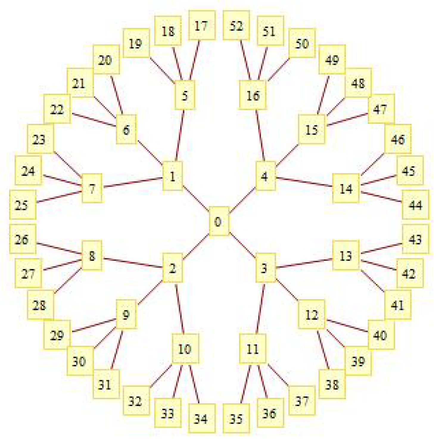
In this section, we develop our theoretical framework in two steps. In the first sub-section, we provide an example of a Dunbar social network graph. The important feature of these graphs is their layerd property. We can then define this class of graphs as an M-polynomial. In the second sub-section, we show how the various CGT topological indices can be derived for graphs of this type.

2.1. The $(m,n,r)$-Agent Recruitment Graph

To provide a concrete example of a Dunbar graph, consider a manager, identified as 0, of an incentive based chain-system marketing business who recruits four agents identified as 1, 2, 3 and 4 under him in his first layer. As per business’s criteria, agent 1 is asked to recruit another three agents under him in second layer, identified as 5, 6 and 7. The same criterion is also applicable for agents 2, 3 and 4. All three agents in the first layer then later recruit another three agents under each of them. Now, each agent of second layer recruits another three agents under him and thus yields a (4, 3, 3)-agent recruitment graph. It provides a suitable description of how a personal social network or a commercial network (such as a recruiting agent’s network in a marketing system) grows over time. Its form represents the state of the network after it has evolved and reached a stable state. Figure 1 illustrates a graph of this type. It provides a suitable description of how a personal social network or a commercial network ( such as a recruiting agents’ network in marketing system) grows over time.

In this section, we define the set of equations that we will use in the following section to calculate the topological indices for various social network graphs.

Now, consider a set of these Dunbar graphs linked through a common individual (or node) at different layers to each other to create a small-world chain. To represent this, we introduce the $(m,n,r)$-agent recruitment graph, where $n>1$, to provide a formal description of this kind of graph as an M-polynomial. This new kind of multi-network (or global network) graph has both M-polynomial and topological indices based on layered structures and the number of agents in each layer. We can therefore derive a set of topological invariants for social networks that relate Dunbar’s Number (represented by the coefficients m and n) to the small-world degrees of separation concept (represented by r).

Definition 1

[38]. Let $G=(V,E)$ be a graph and ${\theta }_{ij}$, $i,j\ge 1$ be the number of edges $e=uv$ of G such that $\{d_u\left(G\right),d_v\left(G\right)\}=\{i,j\}$. Then, M-polynomial of G is $M(G,x,y)$ = $\genfrac{}{}{0pt}{}{\sum }{{}_{i\le j}}$${\theta }_{ij}\left(G\right)x^i{y}^j$.

Following

Table 1. Table of topological index and derivation from $M(G,x,y)$ or $f(x,y)$.

Topological Index	Notion for Topological Index	Derivation from $\mathit{M}(\mathit{G},\mathit{x},\mathit{y})$ or $\mathit{f}(\mathit{x},\mathit{y})$
First Zagreb	$M_1\left(G\right)$	$(D_x+D_y)\left(f(x,y)\right){\mid }_{x=y=1}$
Second Zagreb	$M_2\left(G\right)$	($D_x{D}_y)\left(f(x,y)\right){\mid }_{x=y=1}$
Second modified Zagreb	${}^m$$M_2\left(G\right)$	$S_x{S}_y\left(f(x,y)\right){\mid }_{x=y=1}$
General Randi$\acute{c}$	$R_{\alpha }\left(G\right)$	$D_x^{\alpha }{D}_y^{\alpha }\left(f(x,y)\right){\mid }_{x=y=1}$
General Inverse Randi$\acute{c}$	$R{R}_{\alpha }\left(G\right)$	$S_x^{\alpha }{S}_y^{\alpha }\left(f(x,y)\right){\mid }_{x=y=1}$
Symmetric Division Index	$SDD\left(G\right)$	$(D_x{S}_y+D_y{S}_x)\left(f(x,y)\right){\mid }_{x=y=1}$
Harmonic Index	H(G)	2$S_{x}J\left(f(x,y)\right){\mid }_{x=1}$
Inverse sum Index	I(G)	$S_{x}J{D}_x{D}_y\left(f(x,y)\right){\mid }_{x=1}$
Augmented Zagreb Index	AZI(G)	$S_x^3{Q}_{-2}J{D}_x^3{D}_y^3\left(f(x,y)\right){\mid }_{x=1}$

is due to [38].

According to Deutsch and Kalv$\check{\mathrm{z}}$ar [38], $D_x\left(f(x,y)\right)=x\frac{\partial f(x,y)}{\partial x}$, $D_y\left(f(x,y)\right)=y\frac{\partial f(x,y)}{\partial y}$, $S_x\left(f(x,y)\right)={\int }_o^x$$\frac{f(t,y)}{t}dt$, $S_y\left(f(x,y)\right)={\int }_o^y$$\frac{f(x,t)}{t}dt$, $Q_{\alpha }\left(f(x,y)\right)=x^{\alpha }f(x,y)$ and $\alpha \ne 0$ and $J\left(f\right(x,y\left)\right)=f(x,x)$.

Definition 2.

A graph is said to be $(m,n,r)$-agent recruitment graph, where $n>1$, if it has a vertex of degree m in 1st layer, then each of m vertices has degree n in 2st layer and so on up to $(r-1)$ layer, but degree of each vertex is 1 in $r$ layer.

Figure 1 illustrates a graph of this type. It provides a suitable description of how a personal social network or a commercial network (such as a recruiting agent’s network in a marketing system) grows over time.

If G be any graph, then $V\left(G\right)$ and $E\left(G\right)$ are vertex set and edge set of G respectively. If $\mathcal{G}$ indicates $(m,n,r)$-agent recruitment graph, where $n>1$, then $\left|V\right(\mathcal{G}\left)\right|$ = $1+\frac{m(n^r-1)}{(n-1)}$ and $\left|E\right(\mathcal{G}\left)\right|$ = $\frac{m(n^r-1)}{(n-1)}$.

Now, we have the following

Table 2. Vertex-degree table for $(m,n,r)$-agent recruitment graph.

${\mathit{d}}_{\mathit{u}}$	1	m	$(\mathit{n}+1)$
Number of vertices	$m{n}^{r-1}$	1	$\frac{m(n^{r-1}-1)}{(n-1)}$

and

Table 3. Edge-degree table for $(m,n,r)$-agent recruitment graph.

$({\mathit{d}}_{\mathit{u}},{\mathit{d}}_{\mathit{v}})$	(1, $\mathit{n}+1$)	(m, $\mathit{n}+1$)	($\mathit{n}+1$, $\mathit{n}+1$)
Number of edges	$m{n}^{r-1}$	m	$\frac{mn(n^{r-2}-1)}{(n-1)}$

.

For the sake of easiness of calculations, we denote $\beta =m{n}^{r-1}$, $\gamma =m$ and $\delta =\frac{mn(n^{r-2}-1)}{(n-1)}$.

Let $E_1\left(\mathcal{G}\right),E_2\left(\mathcal{G}\right)$ and $E_3\left(\mathcal{G}\right)$ be the sets of edges $uv\in E\left(\mathcal{G}\right)$ whose incidence vertices have degrees 1 and $n+1$; m and $n+1$; $n+1$ and $n+1$, respectively.

Thus; ${\theta }_{1(n+1)}\left(\mathcal{G}\right)=\mid E_1\left(\mathcal{G}\right)\mid =\beta$, ${\theta }_{m(n+1)}\left(\mathcal{G}\right)=\mid E_2\left(\mathcal{G}\right)\mid =\gamma$ and ${\theta }_{(n+1)(n+1)}\left(\mathcal{G}\right)=\mid E_3\left(\mathcal{G}\right)\mid =\delta$.

Now, due to definition of M-polynomial, we have the following result.

$$\begin{array}{ll}M(\mathcal{G},x,y)& =\sum _{i\le j}{\theta }_{ij}\left(\mathcal{G}\right)x^i{y}^j\\ & ={\theta }_{1(n+1)}\left(\mathcal{G}\right)x{y}^{n+1}+{\theta }_{m(n+1)}\left(\mathcal{G}\right)x^m{y}^{n+1}+{\theta }_{(n+1)(n+1)}\left(\mathcal{G}\right)x^{n+1}{y}^{n+1}\\ & =\beta x{y}^{n+1}+\gamma x^m{y}^{n+1}+\delta x^{n+1}{y}^{n+1}.\end{array}$$

Let, $f(x,y)=M(\mathcal{G},x,y)$. Thus, we have the following results.

$$\begin{array}{ll}{D}_x\left(f(x,y)\right)& =x\frac{\partial \left(f\right(x,y\left)\right)}{\partial x}\\ & =\beta x{y}^{n+1}+m\gamma x^m{y}^{n+1}+(n+1)\delta x^{n+1}{y}^{n+1},\end{array}$$

$$\begin{array}{ll}{D}_y\left(f(x,y)\right)& =y\frac{\partial \left(f\right(x,y\left)\right)}{\partial y}\\ & =\beta (n+1)x{y}^{n+1}+(n+1)\gamma x^m{y}^{n+1}+(n+1)\delta x^{n+1}{y}^{n+1},\end{array}$$

$D_x{D}_y\left(f(x,y)\right)$ = $\beta (n+1)x{y}^{n+1}+\gamma m(n+1)x^m{y}^{n+1}+\delta {(n+1)}^2{x}^{n+1}{y}^{n+1}$,

$$\begin{array}{ll}{S}_x\left(f(x,y)\right)& ={\int }_o^x\frac{f(t,y)}{t}dt\\ & =\beta x{y}^{n+1}+\frac{\gamma }{m}{x}^m{y}^{n+1}+\frac{\delta }{(n+1)}{x}^{n+1}{y}^{n+1},\end{array}$$

$$\begin{array}{ll}{S}_y\left(f(x,y)\right)& ={\int }_o^y\frac{f(x,t)}{t}dt\\ & =\frac{\beta }{(n+1)}x{y}^{n+1}+\frac{\gamma }{(n+1)}{x}^m{y}^{n+1}+\frac{\delta }{(n+1)}{x}^{n+1}{y}^{n+1},\end{array}$$

$$\begin{array}{cc}\hfill S_x{S}_y\left(f(x,y)\right)& =\frac{\beta }{(n+1)}x{y}^{n+1}+\frac{\gamma }{m(n+1)}{x}^m{y}^{n+1}+\frac{\delta }{{(n+1)}^2}{x}^{n+1}{y}^{n+1},\hfill \\ \hfill D_x{S}_y\left(f(x,y)\right)& =\beta (n+1)x{y}^{n+1}+\frac{\gamma (n+1)}{m}{x}^m{y}^{n+1}+\delta x^{n+1}{y}^{n+1},\hfill \\ \hfill D_y{S}_x\left(f(x,y)\right)& =\frac{\beta }{(n+1)}x{y}^{n+1}+\frac{m\gamma }{(n+1)}{x}^m{y}^{n+1}+\delta x^{n+1}{y}^{n+1},\hfill \\ \hfill S_{x}J\left(f(x,y)\right)& =\beta \frac{x^{n+2}}{(n+2)}+\gamma \frac{x^{m+n+1}}{(m+n+1)}+\delta \frac{x^{2(n+1)}}{2(n+1)},\hfill \\ \hfill S_{x}J{D}_x{D}_y\left(f(x,y)\right)& =\frac{\beta (n+1)}{(n+2)}{x}^{n+2}+\frac{\gamma m(n+1)}{(m+n+1)}{x}^{m+n+1}+\frac{\delta {(n+1)}^2}{2(n+1)}{x}^{2(n+1)},\hfill \\ \hfill S_x^3{Q}_{-2}J{D}_x^3{D}_y^3\left(f(x,y)\right)& =\frac{\beta {(n+1)}^3}{n^3}{x}^n+\frac{\gamma m^3{(n+1)}^3}{{(m+n-1)}^3}{x}^{m+n-1}+\frac{\delta {(n+1)}^6}{{\left(2n\right)}^3}{x}^{2n},\hfill \\ \hfill D_x^{\alpha }{D}_y^{\alpha }\left(f(x,y)\right)& =\beta {(n+1)}^{\alpha }x{y}^{n+1}+\gamma m^{\alpha }{(n+1)}^{\alpha }{x}^m{y}^{n+1}+\delta {(n+1)}^{2\alpha }{x}^{n+1}{y}^{n+1},\hfill \\ \hfill S_x^{\alpha }{S}_y^{\alpha }\left(f(x,y)\right)& =\frac{\beta }{{(n+1)}^{\alpha }}x{y}^{n+1}+\frac{\gamma }{m^{\alpha }{(n+1)}^{\alpha }}{x}^m{y}^{n+1}+\frac{\delta }{{(n+1)}^{2\alpha }}{x}^{n+1}{y}^{n+1}.\hfill \end{array}$$

Now, we have the following two results.

$$\begin{array}{c}(D_x{S}_y+D_y{S}_x)\left(f(x,y)\right)=\beta (n+1)x{y}^{n+1}+\frac{\gamma (n+1)}{m}{x}^m{y}^{n+1}+\delta x^{n+1}{y}^{n+1}+\frac{\beta }{(n+1)}x{y}^{n+1}\hfill \\ \hfill +\frac{m\gamma }{(n+1)}{x}^m{y}^{n+1}+\delta x^{n+1}{y}^{n+1},\end{array}$$

$$\begin{array}{c}(D_x+D_y)\left(f(x,y)\right)=\beta x{y}^{n+1}+m\gamma x^m{y}^{n+1}+(n+1)\delta x^{n+1}{y}^{n+1}+\beta (n+1)x{y}^{n+1}+(n+1)\gamma x^m{y}^{n+1}\hfill \\ \hfill +(n+1)\delta x^{n+1}{y}^{n+1}.\end{array}$$

2.2. Topological Indices From The M-polynomial

We can now derive topological indices equivalent to those given in Table 1 for the $(m,n,r)$-agent recruitment graph, where $n>1$. To do this, we set $\beta =m{n}^{r-1}$, $\gamma =m$ and $\delta =\frac{mn(n^{r-2}-1)}{(n-1)}$. We obtain the following topological indices for a $(m,n,r)$-agent recruitment graph, where $n>1$.

Theorem 1.

Let $\mathcal{G}$ be a $(m,n,r)$-agent recruitment graph. Then, $M_1\left(\mathcal{G}\right)$ = $m{n}^{r-1}(n+2)+m(m+n+1)+\frac{mn(n^{r-2}-1)}{(n-1)}(2n+2)$.

Proof. 

We have,

$(D_x+D_y)\left(f(x,y)\right)$ = $\beta x{y}^{n+1}+m\gamma x^m{y}^{n+1}+(n+1)\delta x^{n+1}{y}^{n+1}+\beta (n+1)x{y}^{n+1}+(n+1)\gamma x^m{y}^{n+1}+(n+1)\delta x^{n+1}{y}^{n+1}$.

Hence, $M_1\left(\mathcal{G}\right)$ = $(D_x+D_y)\left(f(x,y)\right){\mid }_{x=y=1}$ = $m{n}^{r-1}(n+2)+m(m+n+1)+\frac{mn(n^{r-2}-1)}{(n-1)}(2n+2)$. ☐

Theorem 2.

Let $\mathcal{G}$ be a $(m,n,r)$-agent recruitment graph. Then, $M_2\left(\mathcal{G}\right)$ = $m{n}^{r-1}(n+1)+m^2(n+1)+\frac{mn(n^{r-2}-1)}{(n-1)}{(n+1)}^2$.

Proof. 

We have,

$D_x{D}_y\left(f(x,y)\right)$ = $\beta (n+1)x{y}^{n+1}+\gamma m(n+1)x^m{y}^{n+1}+\delta {(n+1)}^2{x}^{n+1}{y}^{n+1}$.

Hence, $M_2\left(\mathcal{G}\right)$ = $D_x{D}_y\left(f(x,y)\right){\mid }_{x=y=1}$ = $m{n}^{r-1}(n+1)+m^2(n+1)+\frac{mn(n^{r-2}-1)}{(n-1)}{(n+1)}^2$. ☐

Theorem 3.

Let $\mathcal{G}$ be a $(m,n,r)$-agent recruitment graph. Then, ${}^m$$M_2\left(\mathcal{G}\right)$ = $\frac{m{n}^{r-1}}{(n+1)}+\frac{1}{(n+1)}+\frac{\frac{mn(n^{r-2}-1)}{(n-1)}}{{(n+1)}^2}$.

Proof. 

We have,

$S_x{S}_y\left(f(x,y)\right)$ = $\frac{\beta }{(n+1)}x{y}^{n+1}+\frac{\gamma }{m(n+1)}{x}^m{y}^{n+1}+\frac{\delta }{{(n+1)}^2}{x}^{n+1}{y}^{n+1}$.

Hence, ${}^m$$M_2\left(\mathcal{G}\right)$ = $S_x{S}_y\left(f(x,y)\right){\mid }_{x=y=1}$ = $\frac{m{n}^{r-1}}{(n+1)}+\frac{1}{(n+1)}+\frac{\frac{mn(n^{r-2}-1)}{(n-1)}}{{(n+1)}^2}$. ☐

Theorem 4.

Let $\mathcal{G}$ be a $(m,n,r)$-agent recruitment graph. Then, $R_{\alpha }\left(\mathcal{G}\right)$ = $m{n}^{r-1}{(n+1)}^{\alpha }+m^{1+\alpha }{(n+1)}^{\alpha }+\frac{mn(n^{r-2}-1)}{(n-1)}{(n+1)}^{2\alpha }$, here $\alpha \in N$.

Proof. 

We have,

$D_x^{\alpha }{D}_y^{\alpha }\left(f(x,y)\right)$ = $\beta {(n+1)}^{\alpha }x{y}^{n+1}+\gamma m^{\alpha }{(n+1)}^{\alpha }{x}^m{y}^{n+1}+\delta {(n+1)}^{2\alpha }{x}^{n+1}{y}^{n+1}$.

Hence, $R_{\alpha }\left(\mathcal{G}\right)$ = $D_x^{\alpha }{D}_y^{\alpha }\left(f(x,y)\right){\mid }_{x=y=1}$ = $m{n}^{r-1}{(n+1)}^{\alpha }+m^{1+\alpha }{(n+1)}^{\alpha }+\frac{mn(n^{r-2}-1)}{(n-1)}{(n+1)}^{2\alpha }$, here $\alpha \in N$. ☐

Theorem 5.

Let $\mathcal{G}$ be a $(m,n,r)$-agent recruitment graph. Then, $R{R}_{\alpha }\left(\mathcal{G}\right)$ = $\frac{m{n}^{r-1}}{{(n+1)}^{\alpha }}+\frac{m}{m^{\alpha }{(n+1)}^{\alpha }}+\frac{\frac{mn(n^{r-2}-1)}{(n-1)}}{{(n+1)}^{2\alpha }}$.

Proof. 

We have,

$S_x^{\alpha }{S}_y^{\alpha }\left(f(x,y)\right)$ = $\frac{\beta }{{(n+1)}^{\alpha }}x{y}^{n+1}+\frac{\gamma }{m^{\alpha }{(n+1)}^{\alpha }}{x}^m{y}^{n+1}+\frac{\delta }{{(n+1)}^{2\alpha }}{x}^{n+1}{y}^{n+1}$.

Thus, $R{R}_{\alpha }\left(\mathcal{G}\right)$ = $S_x^{\alpha }{S}_y^{\alpha }\left(f(x,y)\right){\mid }_{x=y=1}$ = $\frac{m{n}^{r-1}}{{(n+1)}^{\alpha }}+\frac{m}{m^{\alpha }{(n+1)}^{\alpha }}+\frac{\frac{mn(n^{r-2}-1)}{(n-1)}}{{(n+1)}^{2\alpha }}$. ☐

Theorem 6.

Let $\mathcal{G}$ be a $(m,n,r)$-agent recruitment graph. Then, $SDD\left(\mathcal{G}\right)$ = $m{n}^{r-1}\{\frac{{(n+1)}^2+1}{n+1}\}+\frac{{(n+1)}^2+m^2}{(n+1)}+2\frac{mn(n^{r-2}-1)}{(n-1)}$.

Proof. 

We have,

$(D_x{S}_y+D_y{S}_x)\left(f(x,y)\right)$ = $\beta (n+1)x{y}^{n+1}+\frac{\gamma (n+1)}{m}{x}^m{y}^{n+1}+\delta x^{n+1}{y}^{n+1}+\frac{\beta }{(n+1)}x{y}^{n+1}+\frac{m\gamma }{(n+1)}{x}^m{y}^{n+1}+\delta x^{n+1}{y}^{n+1}$.

Thus, $SDD\left(\mathcal{G}\right)$ = $(D_x{S}_y+D_y{S}_x)\left(f(x,y)\right){\mid }_{x=y=1}$ = $m{n}^{r-1}\{\frac{{(n+1)}^2+1}{n+1}\}+\{\frac{{(n+1)}^2+m^2}{(n+1)}\}+2\frac{mn(n^{r-2}-1)}{(n-1)}$. ☐

Theorem 7.

Let $\mathcal{G}$ be a $(m,n,r)$-agent recruitment graph. Then, $H\left(\mathcal{G}\right)$ = $\frac{2m{n}^{r-1}}{(n+2)}+\frac{2m}{m+n+1}+\frac{\frac{mn(n^{r-2}-1)}{(n-1)}}{(n+1)}$.

Proof. 

We have,

$S_{x}J\left(f(x,y)\right)$ = $\beta \frac{x^{n+2}}{(n+2)}+\gamma \frac{x^{m+n+1}}{(m+n+1)}+\delta \frac{x^{2(n+1)}}{2(n+1)}$.

Thus, $H\left(\mathcal{G}\right)$ = $S_{x}J\left(f(x,y)\right){\mid }_{x=1}$ = $\frac{2m{n}^{r-1}}{(n+2)}+\frac{2m}{m+n+1}+\frac{\frac{mn(n^{r-2}-1)}{(n-1)}}{(n+1)}$. ☐

Theorem 8.

Let $\mathcal{G}$ be a $(m,n,r)$-agent recruitment graph. Then, $I\left(\mathcal{G}\right)$ = $\frac{m{n}^{r-1}(n+1)}{(n+2)}+\frac{m^2(n+1)}{m+n+1}+\frac{(n+1)\frac{mn(n^{r-2}-1)}{(n-1)}}{2}$.

Proof. 

We have,

$S_{x}J{D}_x{D}_y\left(f(x,y)\right)$ = $\frac{\beta (n+1)}{(n+2)}{x}^{n+2}+\frac{\gamma m(n+1)}{(m+n+1)}{x}^{m+n+1}+\frac{\delta {(n+1)}^2}{2(n+1)}{x}^{2(n+1)}$.

Thus, $I\left(\mathcal{G}\right)$ = $S_{x}J{D}_x{D}_y\left(f(x,y)\right){\mid }_{x=1}$ = $\frac{m{n}^{r-1}(n+1)}{(n+2)}+\frac{m^2(n+1)}{m+n+1}+\frac{(n+1)\frac{mn(n^{r-2}-1)}{(n-1)}}{2}$. ☐

Theorem 9.

Let $\mathcal{G}$ be a $(m,n,r)$-agent recruitment graph. Then, $AZI\left(\mathcal{G}\right)$ = $\frac{m{n}^{r-1}{(n+1)}^3}{n^3}+\frac{m^4{(n+1)}^3}{{(m+n-1)}^3}+\frac{{(n+1)}^6\frac{mn(n^{r-2}-1)}{(n-1)}}{{\left(2n\right)}^3}$.

Proof. 

We have,

$S_x^3{Q}_{-2}J{D}_x^3{D}_y^3\left(f(x,y)\right)$ = $\frac{\beta {(n+1)}^3}{n^3}{x}^n+\frac{\gamma m^3{(n+1)}^3}{{(m+n-1)}^3}{x}^{m+n-1}+\frac{\delta {(n+1)}^6}{{\left(2n\right)}^3}{x}^{2n}$.

Thus, $AZI\left(\mathcal{G}\right)$ = $S_x^3{Q}_{-2}J{D}_x^3{D}_y^3\left(f(x,y)\right){\mid }_{x=1}$ = $\frac{m{n}^{r-1}{(n+1)}^3}{n^3}+\frac{m^4{(n+1)}^3}{{(m+n-1)}^3}+\frac{{(n+1)}^6\frac{mn(n^{r-2}-1)}{(n-1)}}{{\left(2n\right)}^3}$. ☐

3. Dunbar Graphs and Topological Indices

We can now determine the topological indices for a set of graphs that differ in their size and structure in the way we suggested in the Introduction. We consider all possible combinations of m and n values for Dunbar graph layers of 5, 15 and 150, and r = 4 for online social networks and r= 6 for small-world degrees of separation. This is simply a matter of interpolating these values into the equations for Theorems 1–9 in

Table 4. Topological indices of different $(m,n,r)$-agent recruitment graphs.

$(\mathit{m},\mathit{n},\mathit{r})$	${\mathit{M}}_1\left(\mathcal{G}\right)$	${\mathit{M}}_2\left(\mathcal{G}\right)$	${}^{\mathit{m}}$${\mathit{M}}_2\left(\mathcal{G}\right)$	$\mathit{SDD}\left(\mathcal{G}\right)$	$\mathit{H}\left(\mathcal{G}\right)$	$\mathit{I}\left(\mathcal{G}\right)$	$\mathit{AZI}\left(\mathcal{G}\right)$
(5,5,6)	156,230	234,300	2712.6667	96,364.333	5115.1948	5115.1948	13,406.494
(5,150,6)	5.848$\times {10}^{13}$	1.154$\times {10}^{14}$	2.515$\times {10}^9$	5.734$\times {10}^{13}$	5.013$\times {10}^9$	3.772$\times {10}^{11}$	3.873$\times {10}^{11}$.
(5,5,4)	6230	9300	108.5	3864.3333	204.48052	549.35065	1265.1852
(5,150,4)	2.599$\times {10}^9$	5.130$\times {10}^9$	111759.94	2.548$\times {10}^9$	222,789.54	16,764,004	17,215,344
(150,150,6)	1.754$\times {10}^{15}$	3.463$\times {10}^{15}$	7.544$\times {10}^{10}$	1.720$\times {10}^{15}$	1.504$\times {10}^{11}$	1.132$\times {10}^{13}$	1.162$\times {10}^{13}$
(150,150,4)	7.798$\times {10}^{10}$	1.539$\times {10}^{11}$	3352798	7.645$\times {10}^{10}$	6,683,685.2	5.029$\times {10}^8$	5.816$\times {10}^8$
(150,5,6)	470,8650	715,9500	81,375.167	2,894,381	153,430.49	402,651.1	839,940.33
(150,5,4)	208,650	409,500	3250.1667	11,9381	6109.0659	16,936.813	62,340.333
(5,15,6)	73,225,380	1.302$\times {10}^8$	238,364.12	60,987,322	463,641.65	357,3548.5	4,608,373.2
(5,15,4)	325,380	577,600	1059.4375	271,072	2060.7703	15,901.401	20,853.232
(15,5,6)	468,840	703,800	8137.6667	289,106	15,344.286	40,242.857	82,594.256
(15,5,4)	18,840	28,800	325.16667	11,606	612.14286	1671.4286	4834.2557
(15,15,6)	2.197$\times {10}^8$	3.905$\times {10}^8$	715,092.25	1.830$\times {10}^8$	1,390,924.5	10,720,704	13,832,502
(15,15,4)	976,290	1,735,200	3178.1875	813,194.12	6181.8501	47,763.188	69,942.194
(15,150,6)	1.754$\times {10}^{14}$	3.463$\times {10}^{14}$	7.544$\times {10}^9$	1.720$\times {10}^{14}$	1.504$\times {10}^{10}$	1.132$\times {10}^{12}$	1.162$\times {10}^{12}$.
(15,150,4)	7.798$\times {10}^9$	1.539$\times {10}^{10}$	35,279.81	7.645$\times {10}^9$	668,368.6	50,292,145	51,683,780
${\mathit{R}}_{\mathit{\alpha }}\left(\mathcal{G}\right)$				${\mathit{RR}}_{\mathit{\alpha }}\left(\mathcal{G}\right)$
15,625$\times 6^{\alpha }$ + 5${}^{(1+\alpha )}\times$6${}^{\alpha }$ + 3900$\times 6^{2\alpha }$				15625$\times 6^{-\alpha }$ + 5${}^{(1-\alpha )}\times$6${}^{-\alpha }$ + 3900$\times 6^{-2\alpha }$
3.797$\times {10}^{11}$$\times {151}^{\alpha }$ + 5${}^{(1+\alpha )}\times$151${}^{\alpha }$ + 2.548$\times {10}^9$ $\times {151}^{2\alpha }$				3.797$\times {10}^{11}$$\times {151}^{-\alpha }$ + 5${}^{(1-\alpha )}\times$151${}^{-\alpha }$ + 2.548$\times {10}^9$ $\times {151}^{-2\alpha }$
625$\times 6^{\alpha }$ + 5${}^{(1+\alpha )}\times$6${}^{\alpha }$ + 150$\times 6^{2\alpha }$				625$\times 6^{-\alpha }$ + 5${}^{(1-\alpha )}\times$6${}^{-\alpha }$ + 150$\times 6^{-2\alpha }$
16,875,000$\times {151}^{\alpha }$ + 5${}^{(1+\alpha )}\times$151${}^{\alpha }$ + 113,250$\times {151}^{2\alpha }$				16,875,000$\times {151}^{-\alpha }$ + 5${}^{(1-\alpha )}\times$151${}^{-\alpha }$ + 113,250$\times {151}^{-2\alpha }$
1.139$\times {10}^{13}$$\times {151}^{\alpha }$ + 150${}^{(1+\alpha )}\times$151${}^{\alpha }$ + 7.645$\times {10}^{10}$ $\times {151}^{2\alpha }$				1.139$\times {10}^{13}$$\times {151}^{-\alpha }$ + 150${}^{(1-\alpha )}\times$151${}^{-\alpha }$ + 7.645$\times {10}^{10}$ $\times {151}^{-2\alpha }$
5.062$\times {10}^8$$\times {151}^{\alpha }$ + 150${}^{(1+\alpha )}\times$151${}^{\alpha }$ + 3,397,500 $\times {151}^{2\alpha }$				5.062$\times {10}^8$$\times {151}^{-\alpha }$ + 150${}^{(1-\alpha )}\times$151${}^{-\alpha }$ + 3,397,500 $\times {151}^{-2\alpha }$
468,750$\times 6^{\alpha }$ + 150${}^{(1+\alpha )}\times$6${}^{\alpha }$ + 117,000 $\times 6^{2\alpha }$				468,750$\times 6^{-\alpha }$ + 150${}^{(1-\alpha )}\times$6${}^{-\alpha }$ + 117,000 $\times 6^{-2\alpha }$
18,750$\times 6^{\alpha }$ + 150${}^{(1+\alpha )}\times$6${}^{\alpha }$ + 4500 $\times 6^{2\alpha }$				18,750$\times 6^{-\alpha }$ + 150${}^{(1-\alpha )}\times$6${}^{-\alpha }$ + 4500 $\times 6^{-2\alpha }$
3796875$\times {16}^{\alpha }$ + 5${}^{(1+\alpha )}\times$16${}^{\alpha }$ + 271,200 $\times {16}^{2\alpha }$				3,796,875$\times {16}^{-\alpha }$ + 5${}^{(1-\alpha )}\times$16${}^{-\alpha }$ + 271,200 $\times {16}^{-2\alpha }$
16,875$\times {16}^{\alpha }$ + 5${}^{(1+\alpha )}\times$16${}^{\alpha }$ + 1200 $\times {16}^{2\alpha }$				16,875$\times {16}^{-\alpha }$ + 5${}^{(1-\alpha )}\times$16${}^{-\alpha }$ + 1200 $\times {16}^{-2\alpha }$
46,875$\times 6^{\alpha }$ + 15${}^{(1+\alpha )}\times$6${}^{\alpha }$ + 11,700 $\times 6^{2\alpha }$				46,875$\times 6^{-\alpha }$ + 15${}^{(1-\alpha )}\times$6${}^{-\alpha }$ + 11,700 $\times 6^{-2\alpha }$
1875$\times 6^{\alpha }$ + 15${}^{(1+\alpha )}\times$6${}^{\alpha }$ + 450 $\times 6^{2\alpha }$				1875$\times 6^{-\alpha }$ + 15${}^{(1-\alpha )}\times$6${}^{-\alpha }$ + 450 $\times 6^{-2\alpha }$
11,390,625$\times 6^{\alpha }$ + 15${}^{(1+\alpha )}\times$16${}^{\alpha }$ + 813,600 $\times {16}^{2\alpha }$				11,390,625$\times 6^{-\alpha }$ + 15${}^{(1-\alpha )}\times$16${}^{-\alpha }$ + 813,600 $\times {16}^{-2\alpha }$
50,625$\times 6^{\alpha }$ + 15${}^{(1+\alpha )}\times$16${}^{\alpha }$ + 3600 $\times {16}^{2\alpha }$				50,625$\times 6^{-\alpha }$ + 15${}^{(1-\alpha )}\times$16${}^{-\alpha }$ + 3600 $\times {16}^{-2\alpha }$
1.139$\times {10}^{12}$$\times {151}^{\alpha }$ + 15${}^{(1+\alpha )}\times$151${}^{\alpha }$ + 7.645$\times {10}^9$$\times {151}^{2\alpha }$				1.139$\times {10}^{12}$$\times {151}^{-\alpha }$ + 15${}^{(1-\alpha )}\times$151${}^{-\alpha }$ + 7.645$\times {10}^9$$\times {151}^{-2\alpha }$,
50,625,000$\times {151}^{\alpha }$ + 15${}^{(1+\alpha )}\times$151${}^{\alpha }$ + 339,750$\times {151}^{2\alpha }$				50,625,000$\times {151}^{-\alpha }$ + 15${}^{(1-\alpha )}\times$151${}^{-\alpha }$ + 339,750$\times {151}^{-2\alpha }$,

in the form of nine topological indices given in Table 1. We consider first the case of a small-world structure with r = 6 layers. Let, $z=M(\mathcal{G},x,y)$. Now, setting the values of $m=5,n=5$, $r=6$, $-1\le x\le 1$ and $-1\le y\le 1$ in $M(\mathcal{G},x,y)$ we have the following figure of an offline strong supportive Dunbar graph.

The graph in Figure 2 indicates monotonic increasing behaviour of this Dunbar graph with respect to the x-axis and a quadratic relationship with respect to the y-axis.

4. Discussion

We have shown that it is possible to describe the properties of networks using invariants from chemical graph theory. These indices have the benefit that they allow us to capture the dynamic properties of how networks grow, and how information is likely to flow through a network. One of the benefits of an approach based on M-polynomials is that it provides a basis for comparing networks of different size and structure (this being one of the purposes for which these kinds of invariants were originally developed by Randić [31]). For example, extraverts and introverts have networks of different size (with correspondingly different dynamic properties), and M-polynomials provide us with a metric for determining the consequences of these differences both for the personality types concerned and also for their capacity to form integrated networks when their characteristics differ in the way they do.

Of course, social networks differ from chemical molecules in that they are based on patterns of information flow (via social interactions) through a system rather than just electrochemical connections. Nonetheless, the principle is the same, since information can only flow through the connections provided by direct contacts. In that respect, M-polynomials provide us with a natural metric for describing and comparing the structure and properties of social networks in a way that reflects their growth properties. It may also allow us to determine how optimal these networks are, as well as providing a metric for comparing the efficiency of different networks. Such analyses may, for example, have implications for understanding the efficiency of business organizations since these are often based on hierarchically structured networks of this kind [40].

Here, we considered networks with only a limited range of structures. The computed values in Table 4 suggest that networks in which both m and n layers only target their inner core (five) layers are unlikely to reach a wide enough range of alters to successfully meet Milgram’s small-world criterion. So long as all layers at least target their respective 15-layers, a 6-chain path is likely to reach a sufficiently large population to locate the target individual, though 4-chain paths are likely to be challenged. However, both 4- and 6-chain paths are only likely to reach a wide enough population to be sure of finding the target providing all layers exploit their full 150 social network. This confirms the empirical findings of Killworth et al. [41] who used a small-world experimental design to show that the number of people selected as the first step in the chain reached a peak somewhere in the region of 150–250.

5. Conclusions

An exploration of how the M-polynomials change as network size and structure increase allows us to examine how these indices behave. This may allow us to determine which characteristics have most impact on invariants, and so to consider whether it is possible to design networks for administrative structures that are more functional in terms of the efficiency of information flow. This might also have implications for the design of online networking software. We might, for example, ask whether the availability of cheap price service facilities provides the possibility of creating stronger social networks leading to greater social cohesion through shared subgraphs.

References

1. MacCarron, P.; Kaski, K.; Dunbar, R. Calling Dunbar’s number. Soc. Netw. 2016, 47, 151–155. [Google Scholar] [CrossRef]
2. Zhou, W.X.; Sornette, D.; Hill, R.A.; Dunbar, R.I.M. Discrete hierarchical organization of social group sizes. Proc. R. Soc. B 2005, 272, 439–444. [Google Scholar] [CrossRef] [Green Version]
3. Dunbar, R.I.M. The anatomy of friendship. Trends Cognit. Sci. 2018, 22, 32–50. [Google Scholar] [CrossRef]
4. Hill, R.A.; Dunbar, R.I.M. Social network size in humans. Hum. Nat. 2003, 24, 53–72. [Google Scholar] [CrossRef] [PubMed]
5. Arnaboldi, V.; Guazzini, A.; Passarella, A. Egocentric online social networks: Analysis of key features and prediction of tie strength in Facebook. Comput. Commun. 2013, 36, 1130–1144. [Google Scholar] [CrossRef] [Green Version]
6. Chun, H.; Kwak, H.; Eom, Y.H.; Ahn, Y.Y.; Moon, S.; Jeong, H. Comparison of online social relations in terms of volume vs. interaction: A case study of Cyworld. In Proceedings of the IMC-2008, Blagoevgrad, Bulgaria, 25–31 July 2008; pp. 57–69. [Google Scholar]
7. Dunbar, R.I.M. Sexual segregation in human conversations. Behaviour 2016, 153, 1–14. [Google Scholar] [CrossRef]
8. Goncalves, B.; Perra, N.; Vespignani, A. Modeling users’ activity on Twitter networks: Validation. PLoS ONE 2011, 6, e22656. [Google Scholar] [CrossRef] [Green Version]
9. Haerter, J.O.; Jamtveit, B.; Mathiesen, J. Communication dynamics in finite capacity social networks. Phys. Rev. Let. 2012, 109, 168701. [Google Scholar] [CrossRef] [Green Version]
10. Wang, P.; Ma, J.C.; Jiang, Z.Q.; Zhou, W.X.; Sornette, D. Comparative analysis of layered structures in empirical investor networks and cellphone communication networks. EPJ Data 2020, 9, 11, in press. [Google Scholar] [CrossRef]
11. Dunbar, R.I.M. The social brain hypothesis. Evol. Anthropol. 1988, 10, 142–149. [Google Scholar] [CrossRef]
12. Dunbar, R.I.M. Co-evolution of neocortex size, group size and language in humans. Behav. Brain Sci. 1993, 16, 681–734. [Google Scholar] [CrossRef]
13. Wilson, C.; Boe, B.; Sala, A.; Puttaswamy, K.P.N.; Zhao, B.Y. User interactions in social networks and their implications. In Proceedings of the 4th ACM European Conference on Computer Systems (EuroSys ’09), Nuremberg, Germany, 1–3 April 2009. [Google Scholar]
14. Milgram, S. The small-world problem. Psychol. Today 1967, 1, 61–67. [Google Scholar]
15. Barabási, A.L. Linked: The New Science of Networks; Perseus Publishing: Cambridge, MA, USA, 2007; pp. 25–40. [Google Scholar]
16. Travers, J.; Milgram, S. An experimental study of the small-world problem. Sociometry 1969, 32, 425–443. [Google Scholar] [CrossRef]
17. Dodds, P.S.; Muhamad, R.; Watts, D.J. An experimental study of search in global social networks. Science 2003, 301, 827–829. [Google Scholar] [CrossRef] [PubMed] [Green Version]
18. Aylward, B.S.; Odar, C.C.; Kessler, E.D.; Canter, K.S.; Roberts, M.C. Six degrees of separation: An exploratory network analysis of mentoring relationships in pediatric psychology. J. Pediatr. Psychol. 2012, 37, 972–979. [Google Scholar] [CrossRef] [Green Version]
19. Backstrom, L.; Boldi, P.; Rosa, M.; Ugander, J.; Vigna, S. Four degrees of separation. In Proceedings of the 4th Annual ACM Web Science Conference, Evanston, IL, USA, 22–24 June 2012; pp. 33–42. [Google Scholar]
20. Bhagat, S.; Burke, M.; Diuk, C.; Filiz, I.O.; Edunov, S. Three and a Half Degrees of Separation. Available online: https://research.fb.com/three-and-a-half-degrees-of-separation/ (accessed on 18 December 2019).
21. Daraghmi, E.Y.; Yuan, S.M. We are so close, less than 4 degrees separating you and me! Comput. Hum. Behav. 2014, 30, 273–285. [Google Scholar] [CrossRef]
22. Bakhshandeh, R.; Samadi, M.; Azimifar, Z.; Schaeffer, J. Degrees of separation in social networks. In Proceedings of the Symposium on Combinatorial Search, Barcelona, Spain, 15–16 July 2011; pp. 18–23. [Google Scholar]
23. Kalish, Y.; Robins, G. Psychological predispositions and network structure: The relationship between individual predispositions, structural holes and network closure. Soc. Netw. 2006, 28, 56–84. [Google Scholar] [CrossRef]
24. Roberts, S.G.B.; Wilson, R.; Fedurek, P.; Dunbar, R.I.M. Individual differences and personal social network size and structure. Personal. Individ. Differ. 2008, 44, 954–964. [Google Scholar] [CrossRef]
25. Miritello, G.; Lara, R.; Cebrian, M.; Moro, E. Limited communication capacity unveils strategies for human interaction. Sci. Rep. 2013, 3, 1–7. [Google Scholar] [CrossRef] [Green Version]
26. Burch, K.J. Chemical applications of graph theory. In Mathematical Physics in Theoretical Chemistry; Blinder, S.M., House, J.E., Eds.; Elsevier: Amsterdam, The Netherlands, 2019; p. 261. [Google Scholar]
27. Došlić, T. Planer polycyclic graphs and their Tutte polynomials. J. Math. Chem. 2013, 51, 1599–1607. [Google Scholar]
28. Wiener, H.J. Structural Determination of Paraffin Boiling Points. J. Am. Chem. Soc. 1947, 69, 17–20. [Google Scholar] [CrossRef]
29. Zanni, R.; Llompart, M.G.; Domenech, R.G.; Galvez, J. Latest advances in molecular topology applications for drug discovery. Expert Opin. Drug Discov. 2015, 10, 945–957. [Google Scholar] [CrossRef] [PubMed]
30. Munir, M.; Nazeer, W.; Rafique, S.; Kang, S.M. M-polynomial and related topological indices of nanostar dendrimers. Symmetry 2016, 8, 97. [Google Scholar] [CrossRef]
31. Randić, M. Characterization of molecular branching. J. Am. Chem. Soc. 1975, 97, 6609–6615. [Google Scholar] [CrossRef]
32. Bollobas, B.; Erdos, P. Graphs of extremal weights. Ars Comb. 1988, 50, 225–233. [Google Scholar] [CrossRef] [Green Version]
33. Balaban, A.T. Chemical graphs. Theor. Chem. Acta 1979, 53, 355–375. [Google Scholar] [CrossRef]
34. Hosoya, H. On some counting polynomials in chemistry. Discret. Appl. Math. 1988, 19, 239–257. [Google Scholar] [CrossRef] [Green Version]
35. Zhang, H.; Zhang, F. The clar covering polynomial of hexagonal systems I. Discret. Appl. Math. 1996, 69, 147–167. [Google Scholar] [CrossRef]
36. Farrell, E.J. An introduction to matching polynomials. J. Comb. Theor. Ser. B 1979, 27, 75–86. [Google Scholar] [CrossRef] [Green Version]
37. Hassani, F.; Iranmanesh, A.; Mirzaie, S. Schultz and modified Schultz polynomials of C100 fullerene. MATCH Commun. Math. Comput. Chem. 2013, 69, 87–92. [Google Scholar]
38. Deutsch, E.; Klavžar, S. M-Polynomial and degree based topological indices. Iran. J. Math. Chem. 2015, 6, 93–102. [Google Scholar]
39. Yang, H.; Baig, A.Q.; Khalid, W.; Farahani, M.R.; Zhang, X. M-Polynomial and Topological Indices of Benzene Ring Embedded in P-Type Surface Network. J. Chem. 2019, 9. [Google Scholar] [CrossRef]
40. Webber, E.; Dunbar, R.I.M. The fractal structure of communities of practice: Implications for business organization. PLoS ONE 2020, 15, e0232204, in press. [Google Scholar] [CrossRef] [PubMed]
41. Killworth, P.D.; Bernard, H.R.; McCarty, C. Measuring patterns of acquaintanceship. Curr. Anthropol. 1984, 25, 391–397. [Google Scholar] [CrossRef]
42. Dezecache, G.; Dunbar, R. Sharing the joke: The size of natural laughter groups. Evol. Hum. Behav. 2012, 33, 775–779. [Google Scholar] [CrossRef]
43. Dunbar, R.I.M. Constraints on the evolution of social institutions and their implications for information flow. J. Inst. Econ. 2011, 7, 345–371. [Google Scholar] [CrossRef]
44. Dunbar, R.I.M. The social brain: Psychological underpinnings and implications for the structure of organizations. Curr. Dir. Psychol. Sci. 2014, 23, 109–114. [Google Scholar] [CrossRef] [Green Version]
45. Dunbar, R.I.M. Do online social media cut through the constraints that limit the size of offline social networks? R. Soc. Open Sci. 2016, 3, 9. [Google Scholar] [CrossRef] [Green Version]
46. Dunbar, R.I.M.; Duncan, N.D.C.; Nettle, D. Size and structure of freely forming conversational groups. Hum. Nat. 1995, 6, 67–78. [Google Scholar] [CrossRef]
47. Krems, J.; Dunbar, R.I.M. Clique size and network characteristics in hyperlink cinema: Constraints of evolved psychology. Hum. Nat. 2013, 24, 414–429. [Google Scholar] [CrossRef]
48. Krems, J.A.; Dunbar, R.I.M.; Neuberg, S.L. Something to talk about: Are conversation sizes constrained by mental modelling abilities? Evol. Hum. Behav. 2013, 37, 423–428. [Google Scholar] [CrossRef]
49. KremMatthews, P.; Barrett, L. Small-screen social groups: Soap operas and social networks. J. Cult. Evol. Psychol. 2005, 3, 75–86. [Google Scholar]
50. Kwun, Y.C.; Munir, M.; Nazeer, W.; Rafique, S.; Kang, S.M. M-polynomials and topological indices of V-phenylenic nanotubes and nanotori. Sci. Rep. 2017, 7, 1–9. [Google Scholar] [CrossRef] [PubMed] [Green Version]
51. Stiller, J.; Nettle, D.; Dunbar, R.I.M. The small world of Shakespeare’s plays. Hum. Nat. 2004, 14, 397–408. [Google Scholar] [CrossRef] [PubMed]
Figure 1. A ( 4 , 3 , 3 ) -agent recruitment graph.
Symmetry 12 00932 g001
Figure 2. M-polynomial graph of an offline strong supportive Dunbar graph.
Symmetry 12 00932 g002