
Farmland Transfer and Income Distribution Effect of Heterogeneous Farmers with Livelihood Capital: Evidence from CFPS

Abstract
:1. Introduction
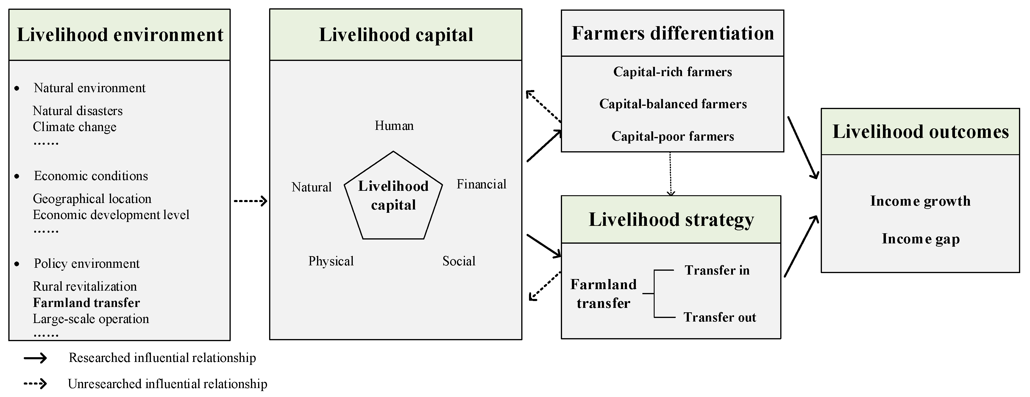
2. Theoretical Framework
2.1. Income Effect of Farmland Transfer
2.2. Income Distribution Effect of Farmland Transfer
2.3. Income Effect of Farmland Transfer of Farmers with Livelihood Capital Heterogeneity
3. Data and Methods
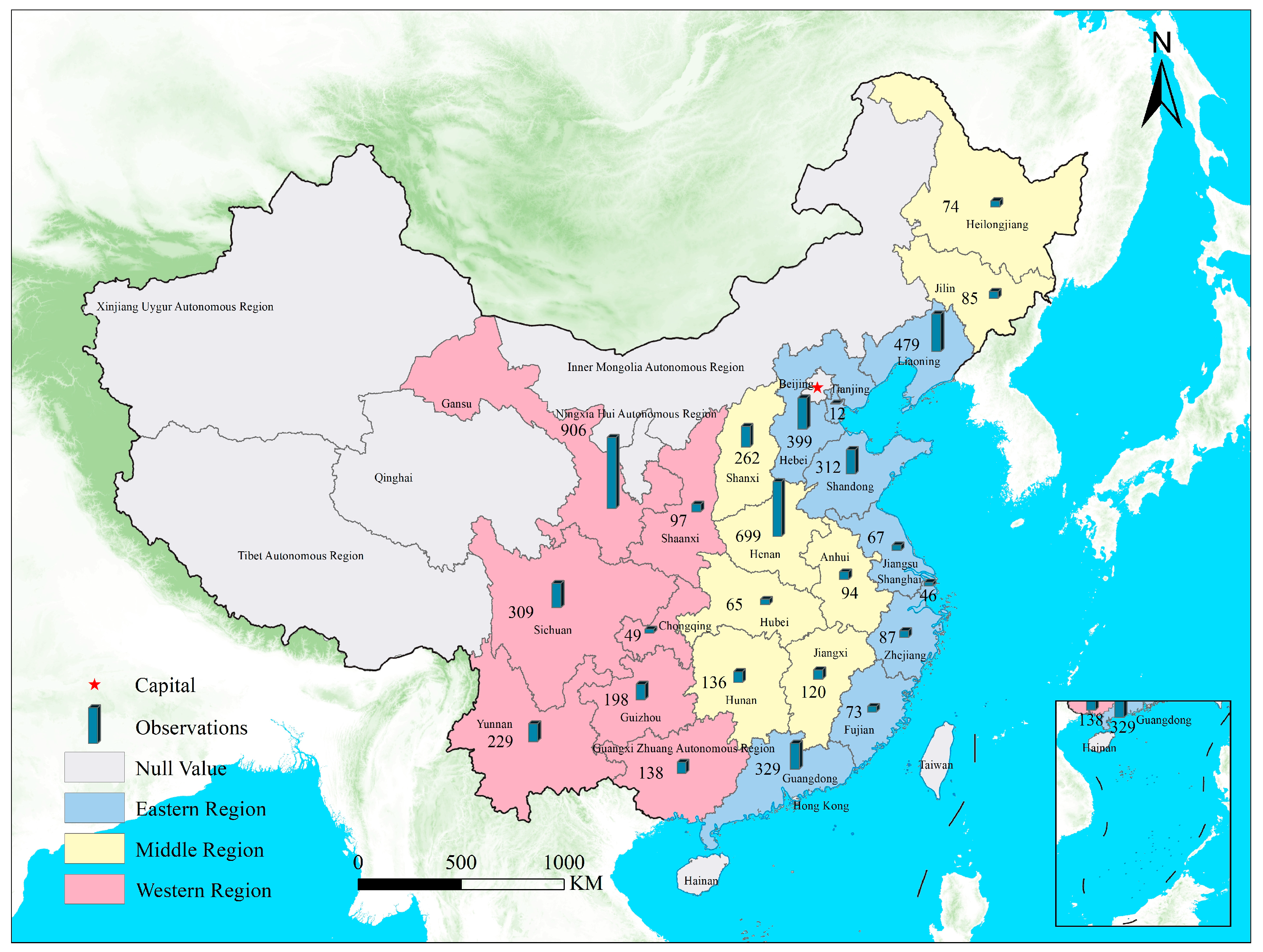
3.1. Data Sources
3.2. Methods
3.2.1. Endogenous Switching Regression Model
3.2.2. Unconditional Quantile Treatment Effect
3.3. Variables
3.3.1. Dependent Variable
3.3.2. Treatment Variable
3.3.3. Instrumental Variable
3.3.4. Control Variable
4. Results
4.1. Influencing Factors of Farmers’ Income
4.2. Impacts of Farmland Transfer on Farmers’ Income
4.3. Impacts of Farmland Transfer on Income Distribution of Farmers
4.4. Income Effects of Farmland Transfer for Heterogeneous Farmers with Livelihood Capital
5. Discussion
6. Conclusions
Author Contributions
Funding
Data Availability Statement
Acknowledgments
Conflicts of Interest
Appendix A
- (1)
- Standardization of raw data.
- (2)
- Calculate the share of the value of the th indicator to the value of the th farmer indicator.
- (3)
- Calculate the entropy value of the th indicator.
- (4)
- Calculate the weight of each indicator.
- (5)
- Measure the total value of farmers’ livelihood capital.
| 1 | The income of farmers in this article is expressed in logarithmic form. The formula used to calculate the growth rate is exp(x) − 1, where x represents the coefficient of the average treatment effect. |
References
- Ghebru, H.; Holden, S. Land rental markets and rural poverty dynamics in Northern Ethiopia: Panel data evidence using survival models. Rev. Dev. Econ. 2018, 23, 131–154. [Google Scholar] [CrossRef] [Green Version]
- Huo, C.; Chen, L. Research on the Impact of Land Circulation on the Income Gap of Rural Households: Evidence from CHIP. Land 2021, 10, 781. [Google Scholar] [CrossRef]
- Li, C.; Jiao, Y.; Sun, T.; Liu, A. Alleviating multi-dimensional poverty through land transfer: Evidence from poverty-stricken villages in China. China Econ. Rev. 2021, 69, 101670. [Google Scholar] [CrossRef]
- Xu, D.; Guo, S.; Xie, F.; Liu, S.; Cao, S. The impact of rural laborer migration and household structure on household land use arrangements in mountainous areas of Sichuan Province, China. Habitat Int. 2017, 70, 72–80. [Google Scholar] [CrossRef]
- Zhang, B.; Niu, W.; Ma, L.; Zuo, X.; Kong, X.; Chen, H.; Zhang, Y.; Chen, W.; Zhao, M.; Xia, X. A company-dominated pattern of land consolidation to solve land fragmentation problem and its effectiveness evaluation: A case study in a hilly region of Guangxi Autonomous Region, Southwest China. Land Use Policy 2019, 88, 104115. [Google Scholar] [CrossRef]
- Xu, L.; Chen, S.; Tian, S. The Mechanism of Land Registration Program on Land Transfer in Rural China: Considering the Effects of Livelihood Security and Agricultural Management Incentives. Land 2022, 11, 1347. [Google Scholar] [CrossRef]
- Huang, K.; Deng, X.; Liu, Y.; Yong, Z.; Xu, D. Does off-Farm Migration of Female Laborers Inhibit Land Transfer? Evidence from Sichuan Province, China. Land 2020, 9, 14. [Google Scholar] [CrossRef] [Green Version]
- Yuan, X.; Du, W.; Wei, X.; Ying, Y.; Shao, Y.; Hou, R. Quantitative analysis of research on China’s land transfer system. Land Use Policy 2018, 74, 301–308. [Google Scholar] [CrossRef]
- Peng, K.; Yang, C.; Chen, Y. Land transfer in rural China: Incentives, influencing factors and income effects. Appl. Econ. 2020, 52, 5477–5490. [Google Scholar] [CrossRef]
- Jin, S.; Jay, T.S. Land Rental Markets in Kenya: Implications for Efficiency, Equity, Household Income, and Poverty. Land Econ. 2013, 89, 246–271. [Google Scholar] [CrossRef]
- Zhang, J.; Mishra, A.K.; Hirsch, S. Market-oriented agriculture and farm performance: Evidence from rural China. Food Policy 2021, 100, 102023. [Google Scholar] [CrossRef]
- Deng, X.; Zhang, M.; Wan, C. The Impact of Rural Land Right on Farmers’ Income in Underdeveloped Areas: Evidence from Micro-Survey Data in Yunnan Province, China. Land 2022, 11, 1780. [Google Scholar] [CrossRef]
- Udimal, T.B.; Liu, E.; Luo, M.; Li, Y. Examining the effect of land transfer on landlords’ income in China: An application of the endogenous switching model. Heliyon 2020, 6, e05071. [Google Scholar] [CrossRef] [PubMed]
- Guo, J.; Qu, S.; Xia, Y.; Lv, K. Income distribution effect of rural land transfer. China Popul. Resour. Environ. 2018, 28, 160–169. [Google Scholar]
- Chen, L.; Chen, H.; Zou, C.; Liu, Y. The Impact of Farmland Transfer on Rural Households’ Income Structure in the Context of Household Differentiation: A Case Study of Heilongjiang Province, China. Land 2021, 10, 362. [Google Scholar] [CrossRef]
- Peng, D.; Wu, Y. An empirical test of the relation between concentration of farmland and increase of farmers’ income. Chin. Rural. Econ. 2009, 4, 17–22. [Google Scholar]
- Zhu, J.; Hu, J. A Study on the impact of farmland circulation on the income distribution of Chinese farmers—Based on the data of China’s health and pension tracking survey. Nanjing Agric. Univ. (Soc. Sci. Ed.) 2015, 15, 75–83. [Google Scholar]
- Shi, C.; Luan, J.; Zhu, J.; Chen, Y. Land transaction and farmers’income:an analysis based on chinese eight provinces survey data. Econ. Rev. 2017, 5, 152–166. [Google Scholar]
- Jin, S.; Deininger, K. Land rental markets in the process of rural structural transformation: Productivity and equity impacts from China. J. Comp. Econ. 2009, 37, 629–646. [Google Scholar] [CrossRef] [Green Version]
- Zhang, Q. Retreat from Equality or Advance towards Efficiency? Land Markets and Inequality in Rural Zhejiang. China Q. 2008, 195, 535–557. [Google Scholar] [CrossRef]
- Deinnger, K. Making Negotiated Land Reform Work: Initial Experience from Colombia, Brazil and South Africa. World Dev. 1999, 27, 651–672. [Google Scholar] [CrossRef]
- Begazo Curie, K.; Mertens, K.; Vranken, L. Tenure regimes and remoteness: When does forest income reduce poverty and inequality? A case study from the Peruvian Amazon. For. Policy Econ. 2021, 128, 102478. [Google Scholar] [CrossRef]
- Magnan, A.; Davidson, M.; Desmarais, A.A. ‘They call it progress, but we don’t see it as progress’: Farm consolidation and land concentration in Saskatchewan, Canada. Agric. Hum. Values 2022, 40, 277–290. [Google Scholar] [CrossRef]
- Gao, X.; Zhang, A.; Yang, X.; Li, C. Farmers’ income and income distribution effect of farmland transfer: A case study on 5 cites in Hunan province. China Land Sci. 2016, 30, 48–56. [Google Scholar]
- Yang, H.; Huang, K.; Deng, X.; Xu, D. Livelihood Capital and Land Transfer of Different Types of Farmers: Evidence from Panel Data in Sichuan Province, China. Land 2021, 10, 532. [Google Scholar] [CrossRef]
- Xu, D.; Deng, X.; Guo, S.; Liu, S. Sensitivity of Livelihood Strategy to Livelihood Capital: An Empirical Investigation Using Nationally Representative Survey Data from Rural China. Soc. Indic. Res. 2018, 144, 113–131. [Google Scholar] [CrossRef]
- Wang, P.; Yan, J.; Hua, X.; Yang, L. Determinants of livelihood choice and implications for targeted poverty reduction policies: A case study in the YNL river region, Tibetan Plateau. Ecol. Indic. 2019, 101, 1055–1063. [Google Scholar] [CrossRef]
- Singh, P.K.; Hiremath, B.N. Sustainable livelihood security index in a developing country: A tool for development planning. Ecol. Indic. 2010, 10, 442–451. [Google Scholar] [CrossRef]
- Ellis, F.; Bahiigwa, G. Livelihoods and Rural Poverty Reduction in Uganda. World Dev. 2003, 31, 997–1013. [Google Scholar] [CrossRef]
- Baffoe, G.; Matsuda, H. An empirical assessment of rural livelihood assets from gender perspective: Evidence from Ghana. Sustain. Sci. 2017, 13, 815–828. [Google Scholar] [CrossRef]
- Yang, L.; Liu, M.; Lun, F.; Min, Q.; Li, W. The impacts of farmers’ livelihood capitals on planting decisions: A case study of Zhagana Agriculture-Forestry-Animal Husbandry Composite System. Land Use Policy 2019, 86, 208–217. [Google Scholar] [CrossRef]
- Hahn, M.B.; Riederer, A.M.; Foster, S.O. The Livelihood Vulnerability Index: A pragmatic approach to assessing risks from climate variability and change—A case study in Mozambique. Glob. Environ. Chang. 2009, 19, 74–88. [Google Scholar] [CrossRef]
- The UK’s Department for International Development. Sustainable Livelihoods Guidance Sheets; DFID: London, UK, 1999; p. 445. [Google Scholar]
- Soini, E. Land use change patterns and livelihood dynamics on the slopes of Mt. Kilimanjaro, Tanzania. Agric. Syst. 2005, 85, 306–323. [Google Scholar] [CrossRef] [Green Version]
- Zhang, J.; Mishra, A.K.; Zhu, P.; Li, X. Land rental market and agricultural labor productivity in rural China: A mediation analysis. World Dev. 2020, 135, 105089. [Google Scholar] [CrossRef]
- Liu, Z.; Zhang, L.; Rommel, J.; Feng, S. Do land markets improve land-use efficiency? Evidence from Jiangsu, China. Appl. Econ. 2019, 52, 317–330. [Google Scholar] [CrossRef]
- Mao, P.; Xu, J. The system of the farmland, the transfer of the right of the land operation, and the growth of farmers’ income. J. Manag. World 2015, 5, 63–74, 88. [Google Scholar]
- Zhang, X.; Yu, X.; Tian, X.; Geng, X.; Zhou, Y. Farm size, inefficiency, and rice production cost in China. J. Product. Anal. 2019, 52, 57–68. [Google Scholar] [CrossRef]
- Lu, H.; Xie, H.; Yao, G. Impact of land fragmentation on marginal productivity of agricultural labor and non-agricultural labor supply: A case study of Jiangsu, China. Habitat Int. 2019, 83, 65–72. [Google Scholar] [CrossRef]
- Xie, H.; Lu, H. Impact of land fragmentation and non-agricultural labor supply on circulation of agricultural land management rights. Land Use Policy 2017, 68, 355–364. [Google Scholar] [CrossRef]
- Deininger, K.; Jin, S. The potential of land rental markets in the process of economic development: Evidence from China. J. Dev. Econ. 2005, 78, 241–270. [Google Scholar] [CrossRef]
- Chamberlin, J.; Ricker-Gilbert, J. Participation in Rural Land Rental Markets in Sub-Saharan Africa: Who Benefits and by How Much? Evidence from Malawi and Zambia. Am. J. Agric. Econ. 2016, 98, 1507–1528. [Google Scholar] [CrossRef] [Green Version]
- Liu, H. A study of increases of rural income for farmers whose collective agricultural lands being transferred: A case study of the government-led farmland transfer model. Rural. Econ. 2010, 7, 57–61. [Google Scholar]
- Han, H.; Zhong, F. The impacts of flow direction of “surplus farmland” left by out-flowing rural labours on local farmers’ income distribution. Chin. Rural. Econ. 2011, 4, 18–25. [Google Scholar]
- Leng, Z.; Fu, C.; Xu, X. Family income structure, income gap, and land circulation: A microscopic analysis based on CFPS data. Econ. Rev. 2015, 5, 111–128. [Google Scholar]
- Xiao, L.; Zhang, B. Land transfer and expansion of rural residents’ income gap: Based on the survey of 725 farmers from 39 villages in Jiangsu Province. Collect. Essays Financ. Econ. 2017, 9, 10–18. [Google Scholar]
- Wang, W.; Gong, J.; Wang, Y.; Shen, Y. Exploring the effects of rural site conditions and household livelihood capitals on agricultural land transfers in China. Land Use Policy 2021, 108, 105523. [Google Scholar] [CrossRef]
- Dib, J.B.; Alamsyah, Z.; Qaim, M. Land-use change and income inequality in rural Indonesia. For. Policy Econ. 2018, 94, 55–66. [Google Scholar] [CrossRef]
- Heineck, G.; Anger, S. The returns to cognitive abilities and personality traits in Germany. Labour Econ. 2010, 17, 535–546. [Google Scholar] [CrossRef] [Green Version]
- Huang, J.; Gao, L.; Ji, X.; Scott, R. Farmland System, Farmland Transfer and Farmland Investment in China; Shanghai People’s Publishing House: Shanghai, China, 2012; p. 170. [Google Scholar]
- Wang, W.; Gong, J.; Wang, Y.; Shen, Y. The Causal Pathway of Rural Human Settlement, Livelihood Capital, and Agricultural Land Transfer Decision-Making: Is It Regional Consistency? Land 2022, 11, 1077. [Google Scholar] [CrossRef]
- Lee, L.-F. Some approaches to the correction of selectivity Bias. Rev. Econ. Stud. 1982, 49, 355–372. [Google Scholar] [CrossRef] [Green Version]
- Frölich, M.M.B. Estimation of quantile treatment effects with Stata. Stata J. 2010, 10, 423–457. [Google Scholar] [CrossRef] [Green Version]
- Zhu, P.F.D.J.P. Unconditional quantile treatment effects and application in policy evaluation. J. Quant. Tech. Econ. 2017, 34, 139–155. [Google Scholar]
- Frölich, M.; Melly, B. Unconditional Quantile Treatment Effects Under Endogeneity. J. Bus. Econ. Stat. 2013, 31, 346–357. [Google Scholar] [CrossRef] [Green Version]
- Sergio, F. Efficient Semiparametric Estimation of Quantile Treatment Effects. Econometrica 2007, 75, 259–276. [Google Scholar]
- Chen, F.; Zhai, W. Land transfer incentive and welfare effect research from perspective of farmers’ behavior. Econ. Res. J. 2015, 50, 163–177. [Google Scholar]
- Chen, Y.Y.; Fu, W. Land contract right circulation, labor migration and agriculture production. J. Manag. World 2017, 11, 79–93. [Google Scholar]
- Jezeer, R.E.; Verweij, P.A.; Boot, R.G.A.; Junginger, M.; Santos, M.J. Influence of livelihood assets, experienced shocks and perceived risks on smallholder coffee farming practices in Peru. J. Environ. Manag. 2019, 242, 496–506. [Google Scholar] [CrossRef] [Green Version]
- Barrera-Mosquera, V.; de los Rios-Carmenado, I.; Cruz-Collaguazo, E.; Coronel-Becerra, J. Analysis of available capitals in agricultural systems in rural communities: The case of Saraguro, Ecuador. Span. J. Agric. Res. 2018, 8, 1191–1207. [Google Scholar] [CrossRef] [Green Version]
- Zhang, L.; Feng, S.; Heerink, N.; Qu, F.; Kuyvenhoven, A. How do land rental markets affect household income? Evidence from rural Jiangsu, P.R. China. Land Use Policy 2018, 74, 151–165. [Google Scholar] [CrossRef]
- Liu, M.; Yang, L.; Bai, Y.; Min, Q. The impacts of farmers’ livelihood endowments on their participation in eco-compensation policies: Globally important agricultural heritage systems case studies from China. Land Use Policy 2018, 77, 231–239. [Google Scholar] [CrossRef]
- Guan, R.; Wang, W.L.; Yu, J. Impact of endogenous motivation on household income under the framework of sustainable livelihoods. J. Northwest AF Univ. (Soc. Sci. Ed.) 2019, 19, 130–139. [Google Scholar]
- Wang, J. Village non-agriculturization, social capital and rural household income. J. South China Agric. Univ. (Soc. Sci. Ed.) 2019, 18, 71–83. [Google Scholar]
- Tikadar, K.K.; Islam, M.J.; Saha, S.M.; Alam, M.M.; Barman, S.K.; Rahman, M.A. Livelihood status of small-scale fishermen and determinants of their income: Insights from north-eastern floodplains of Bangladesh. Geogr. Sustain. 2022, 3, 204–213. [Google Scholar] [CrossRef]


| Variable Type | Variables | Date Sources | Year |
|---|---|---|---|
| Dependent variable | Household income | Family database | 2018 |
| Treatment variable | Farmland transfer | Family database | 2018 |
| Control variable | Livelihood capital | Family database | 2012 |
| Village and region | Community database | 2014 |
| Variables | Definition of Variables | Mean | SD |
|---|---|---|---|
| Dependent variable | |||
| Income | Per capita net income of household (yuan/person) | 18,110.47 | 54,158.19 |
| Treatment variable | |||
| Farmland transfer-in | Transferring in farmland (=1 if farmer transfers in land; 0 otherwise) | 0.111 | 0.315 |
| Farmland transfer-out | Transferring out farmland (=1 if farmer transfers out land; 0 otherwise) | 0.173 | 0.378 |
| Natural capital | |||
| Land area | Family contracted land area (mu 1) | 10.291 | 31.711 |
| Human capital | |||
| Labor | Number of labor force in households between 16–60 years old (person) | 3.028 | 1.215 |
| Education level | Average education level of household labor force (year) | 7.079 | 3.143 |
| Physical capital | |||
| Agricultural machinery | Total value of agricultural equipment (yuan) | 1691.441 | 6413.613 |
| House | The market value of currently occupied housing (yuan) | 111,733.8 | 203,327.5 |
| Financial capital | |||
| Deposits | Total household cash and savings (yuan) | 15,389.55 | 35,592.97 |
| Borrowing capacity | Ability to obtain loans from banks or informal financial institutions (=1 if farmer can access loans; 0 otherwise) | 0.363 | 0.481 |
| Social capital | |||
| Relatives | Participating in ancestor worship and tomb-sweeping activities (=1 if farmer Participates; 0 otherwise) | 0.691 | 0.462 |
| Relational network | Household expenditure on economic transactions with non-resident relatives (yuan) | 800.51 | 4028.15 |
| Village and regional variable | |||
| Village location | The distance between village and county town (li 2) | 52.621 | 41.717 |
| Village economic condition | Very Poor --1--2--3--4--5--6--7--> very rich | 3.837 | 1.259 |
| Middle 3 | Middle region = 1, else = 0 | 0.292 | 0.455 |
| Western 4 | Western region = 1, else = 0 | 0.366 | 0.482 |
| Instrumental variables | |||
| Village farmland transfer ratio | The ratio of land circulation in the village (%) | 0.512 | 0.500 |
| Village farmland transfer degree | high ratio = 1, low ratio = 0 | 0.255 | 0.187 |
| Variables | Model 1 | Model 2 | Model 3 | Model 4 | Model 5 | Model 6 |
|---|---|---|---|---|---|---|
| Transferred-In Households | Non-Transferred-In Households | Selection Model of Farmland Transfer-In | Transferred-Out Households | Non-Transferred-Out Households | Selection Model of Farmland Transfer-Out | |
| Land area (log) | 0.077 (0.050) | −0.050 *** (0.016) | −0.038 (0.026) | −0.037 (0.039) | −0.031 * (0.016) | −0.033 (0.023) |
| Labor | −0.041 (0.039) | 0.015 (0.012) | 0.035 * (0.020) | 0.062 ** (0.030) | 0.019 (0.013) | −0.053 *** (0.018) |
| Education level | 0.099 *** (0.016) | 0.065 *** (0.005) | −0.020 ** (0.008) | 0.023 * (0.012) | 0.064 *** (0.005) | 0.033 *** (0.007) |
| Agricultural machinery (log) | −0.044 *** (0.013) | −0.000 (0.004) | 0.044 *** (0.006) | 0.013 (0.010) | 0.006 (0.004) | −0.021 *** (0.006) |
| House (log) | −0.005 (0.020) | 0.025 *** (0.006) | 0.001 (0.010) | 0.027 ** (0.012) | 0.020 *** (0.006) | −0.002 (0.008) |
| Deposits (log) | 0.014 (0.017) | 0.028 *** (0.005) | 0.010 (0.009) | 0.046 *** (0.013) | 0.021 *** (0.006) | 0.006 (0.008) |
| Borrowing capacity | −0.115 (0.095) | 0.028 (0.031) | 0.213 *** (0.050) | 0.091 (0.074) | 0.047 (0.032) | −0.023 (0.045) |
| Relatives | 0.028 (0.097) | 0.057 * (0.031) | −0.017 (0.051) | −0.125 (0.077) | 0.068 ** (0.032) | 0.070 (0.046) |
| Relational network (log) | −0.014 (0.014) | 0.022 *** (0.005) | 0.005 (0.008) | 0.026 ** (0.011) | 0.015 *** (0.005) | 0.002 (0.007) |
| Village location (log) | −0.042 (0.057) | −0.041 ** (0.016) | −0.005 (0.028) | 0.046 (0.040) | −0.052 *** (0.017) | −0.021 (0.024) |
| Village economic condition | 0.099 *** (0.036) | 0.052 *** (0.012) | −0.004 (0.019) | −0.048 (0.029) | 0.055 *** (0.012) | 0.089 *** (0.017) |
| Village farmland transfer ratio | 0.875 *** (0.111) | 0.913 *** (0.108) | ||||
| Middle | −0.177 (0.113) | −0.113 *** (0.036) | 0.151** (0.059) | −0.064 (0.088) | −0.075** (0.037) | −0.006 (0.053) |
| Western | −0.073 (0.119) | −0.046 (0.036) | 0.023 (0.062) | −0.258 *** (0.086) | 0.007 (0.039) | 0.049 (0.053) |
| Constant | 10.826 *** (0.427) | 8.283 *** (0.114) | −1.710 *** (0.196) | 10.177 *** (0.331) | 8.290 *** (0.121) | −1.507 *** (0.172) |
| ρ1 | −1.408 *** (0.107) | −1.159 *** (0.117) | ||||
| ρ2 | −0.122 * (0.073) | −0.097 (0.072) | ||||
| Observations | 5265 | 5265 | 5265 | 5265 | 5265 | 5265 |
| Log likelihood | −8963.5611 | −9515.2413 | ||||
| Wald chi2 | 79.03 *** | 59.99 *** | ||||
| LR chi2 | 41.07 *** | 23.45 *** | ||||
| Farmers’ Type | Actual Outcome | Counterfactual Outcome | ATT |
|---|---|---|---|
| Transferred-in | 9.308 (0.015) | 9.060 (0.013) | 0.248 *** (0.010) |
| Transferred-out | 9.533 (0.012) | 9.173 (0.010) | 0.360 *** (0.007) |
| Quantile | Farmland Transfer-In | Farmland Transfer-Out |
|---|---|---|
| τ = 0.2 | 0.683 (0.974) | 0.716 (0.741) |
| τ = 0.4 | 0.695 *** (0.181) | 1.167 *** (0.242) |
| τ = 0.6 | 0.836 *** (0.309) | 1.306 *** (0.383) |
| τ = 0.8 | 1.267 *** (0.439) | 1.129 ** (0.458) |
| Farmers’ Type | Observations | Natural Capital | Human Capital | Physical Capital | Financial Capital | Social Capital | Livelihood Capital |
|---|---|---|---|---|---|---|---|
| Livelihood capital-rich | 1775 | 0.0117 | 0.3372 | 0.0142 | 0.4653 | 0.1163 | 0.9447 |
| Livelihood capital-balanced | 1929 | 0.0086 | 0.3342 | 0.0127 | 0.0601 | 0.1145 | 0.5301 |
| Livelihood capital-poor | 1561 | 0.0074 | 0.2050 | 0.0071 | 0.0061 | 0.0628 | 0.2884 |
| Total sample | 5265 | 0.0093 | 0.2969 | 0.0116 | 0.1807 | 0.0998 | 0.5982 |
| F | 10.16 | 912.43 | 43.85 | 11,002.03 | 323.13 | 16,812.52 | |
| Prob > F | 0.0000 | 0.0000 | 0.0000 | 0.0000 | 0.0000 | 0.0000 |
| Farmland Transfer Decision | Farmers’ Type | Observations of Farmland Transfer | Actual Outcome | Counterfactual Outcome | ATT |
|---|---|---|---|---|---|
| Transfer-in | Livelihood capital-rich | 238 | 9.464 (0.021) | 9.154 (0.015) | 0.310 *** (0.021) |
| Livelihood capital-balanced | 203 | 9.269 (0.032) | 9.075 (0.022) | 0.194 *** (0.023) | |
| Livelihood capital-poor | 145 | 9.070 (0.024) | 8.910 (0.029) | 0.160 *** (0.026) | |
| Transfer-out | Livelihood capital-rich | 300 | 9.559 (0.021) | 9.355 (0.011) | 0.204 *** (0.013) |
| Livelihood capital-balanced | 355 | 9.664 (0.016) | 9.143 (0.019) | 0.521 *** (0.009) | |
| Livelihood capital-poor | 256 | 9.312 (0.018) | 8.931 (0.019) | 0.381 *** (0.014) |
Disclaimer/Publisher’s Note: The statements, opinions and data contained in all publications are solely those of the individual author(s) and contributor(s) and not of MDPI and/or the editor(s). MDPI and/or the editor(s) disclaim responsibility for any injury to people or property resulting from any ideas, methods, instructions or products referred to in the content. |
© 2023 by the authors. Licensee MDPI, Basel, Switzerland. This article is an open access article distributed under the terms and conditions of the Creative Commons Attribution (CC BY) license (https://creativecommons.org/licenses/by/4.0/).
Share and Cite
Wang, X.; Xu, Z.; Li, G.; Zhuo, Y.; Zou, W. Farmland Transfer and Income Distribution Effect of Heterogeneous Farmers with Livelihood Capital: Evidence from CFPS. Land 2023, 12, 1398. https://doi.org/10.3390/land12071398
Wang X, Xu Z, Li G, Zhuo Y, Zou W. Farmland Transfer and Income Distribution Effect of Heterogeneous Farmers with Livelihood Capital: Evidence from CFPS. Land. 2023; 12(7):1398. https://doi.org/10.3390/land12071398
Chicago/Turabian StyleWang, Xueqi, Zhongguo Xu, Guan Li, Yuefei Zhuo, and Wei Zou. 2023. "Farmland Transfer and Income Distribution Effect of Heterogeneous Farmers with Livelihood Capital: Evidence from CFPS" Land 12, no. 7: 1398. https://doi.org/10.3390/land12071398