Analysis of Ecosystem Service Contribution and Identification of Trade-Off/Synergy Relationship for Ecosystem Regulation in the Dabie Mountains of Western Anhui Province, China

Abstract

The study of tradeoffs/synergies among ecosystem services (ESs) is highly significant for land-use planning and regional ecosystem optimization. Land-use change and topographic factors have important implications for ESs. Strengthening the comparative analysis of the capacity of ESs provided by different land-use types in specific regions, studying the topographic gradient effects of ecosystem service trade-offs/synergies with slope changes, and identifying the dominate trade-off/synergy relationship among ESs will help us to carry out ecosystem regulation according to local conditions through land-use layout optimization at a fine scale. Our research site was located in the Dabie Mountains of western Anhui Province, China (DBM), where, based on the InVEST software, R language, self-organizing maps (SOM), and GeoDA, the temporal and spatial variations of five typical ESs, including food supply, soil retention, water yield, carbon storage, and biodiversity maintenance from 2005 to 2020, were analyzed, and spatial distributions of the different ESs clusters were also recognized by using the SOM method. Moreover, the impacts of land-use type and slope on ESs, and the characteristics of trade-offs/synergies among the five ESs, were discussed. Results showed, firstly, that the total values of ESs showed a changing trend of “three increases and two decreases” from 2005 to 2020. Among the ESs, food supply, soil retention and water yield showed upward trends, with annual growth rates of 2.83%, 6.50% and 2.98%, respectively, whereas carbon storage and biodiversity maintenance showed downward trends, with annual decline rates of 0.03% and 0.07%, respectively. Second, the results showed that the Moran’s I index of the total ESs was 0.3995 in 2005 and 0.4305 in 2020, respectively, indicating that they had significant spatial clustering characteristics. The Low-Low clustering regions with reduced changes were mainly in the central and northern parts of the study area, whereas the High-High clustering regions with increased changes were found distributed mainly in the south of the study area. Thirdly, it was found that cropland and woodland were the main contributors to the total amounts of ESs, but the supply capacity of ESs per unit area of woodland was the largest, constituting nearly 1/3 of the total supply capacity of the ESs. Last, the slope effect on trade-offs and synergies was significant between typical ecosystem service pairs in the study area; trade-offs were the main relationships between the pairs of ESs in the study area, which accounted for nearly 60% of all types of trade-offs/synergies during the 15 years. In addition, the spatial distributions of the trade-offs/synergies between ESs pairs were visualized clearly, and the six ES bundles were identified by using the SOM method at the township administrative scale. The identification of ecosystem service bundles is of great significance for the division of ecological functional zones and ecological regulation in the DBM.

1. Introduction

Ecosystem services (ESs) are life-support products and services that can be obtained directly or indirectly through the structure, processes, and functions of the ecosystem to maintain the natural environmental conditions and utilities on which human beings depend [1]. Land-use change is an important driver of ecosystem service transformation [2]. Currently, nearly 60% of ESs have been partially or fully diminished due to irrational land use [3]. Rational land-use planning utilizes the spatial relationship between ESs towards synergistic optimization [4,5]. The scientific assessment of ESs has gradually become an important prerequisite for the formulation of ecological protection policy objectives, the determination of ecological compensation models, and the precise regulation and control of ecosystems. Studies have shown that ESs have provided a scientific basis for ecosystem management at the national and regional scales [6,7]. At present, research on ESs mainly focuses on the calculation of ES value, the assessment of ecosystem service supply and demand [8], ecosystem service flows [9], and the collaborative research on the relationship between ESs and human wellbeing [10,11]. ES assessment and trade-offs/synergies research provide comprehensive and practical methods for addressing the environmental challenges faced in development [12]. They also offer an important practical field for research on the core proposition of the relationship between man and land in geography [13,14].

The diversity of ecosystem service types, the spatial heterogeneity of ESs, and human management lead to nonlinear and complex interactions among ESs [15,16]. Thus, uncovering the complex interactions and identifying the dominating types of trade-offs and synergies among ESs constitute the basis and premise for sustainable ecosystem management [17,18,19]. Presently, many methods, such as correlation analysis [20] and Bayesian belief networks [21], have been applied to uncover the pairs of trade-offs/synergies relationships among ESs. Meanwhile, spatial autocorrelation analysis [22], the spatial mapping of ESs evaluation [23], and the geographically weighted regression (GWR) [24] are methods commonly used to study the spatial distribution characteristics of ESs. Furthermore, a growing number of recent studies have used the structural equation model (SEM) [25] and self-organizing maps (SOM) [26] to analyze ES bundles, and some new indicators, such as [27] the trade-off/synergy criteria (TSC) and trade-off/synergy index (TSI), have been designed to measure the strength of trade-offs and synergies between ESs. The method of multiple scenarios [28] has also been used to simulate the impact of land-use change on ESs. However, some of these recent studies were still limited to static assessments at a single time or spatial scale [26]. Realizing the trade-off/synergy effect of ESs is fundamental to achieving efficient ecosystem management and improved human wellbeing. Yet current research addressing the driving mechanisms behind the formation of ecosystem service relationships remains limited [29]. Strengthening the study of ecosystem service bundles can effectively reflect the interdependence of ESs, which is important for ecosystem regulation decisions [30]. ES model and method integration and algorithm design are important ways to research trade-off mechanisms and multi-dimensional and complex ESs [31,32]. Therefore, it is necessary to research the spatiotemporal variation and multi-scale characterization of ecosystem service interactions. For regions with complex terrain, it is valuable to pay attention to the sensitivity of the interaction between ESs to terrain differences. Identifying the dominant relationship between ecosystem service trade-offs/synergies is also key to the precise regulation of regional ecosystem functions. In addition, the analysis of ecosystem service contribution rates for different land types can clarify the composition of ecosystem service contributions for different land types, thereby contributing to land-use management and optimization, and ultimately effectively improving the value of regional ESs.

The DBM is famous as a region with history and culture and rich tourism resources which enjoys a winning reputation internationally. In 2018, UNESCO approved the Dabie Mountain Geopark as a world geopark. We all know that targeted poverty alleviation is a great livelihood project in China and in the world, and the DBM is a core area for taking targeted measures in poverty alleviation which has received wide attention from scholars because of its unique location, geological landscape, and history and culture in recent years [33,34]. Therefore, it is important to strengthen research on ecosystem service assessment, contribution sources, and trade-off/synergy interactions in the DBM for ecosystem regulation and the enhancement of ecosystem service values here. With the complex topography of the DBM, the optimization of ecosystem function is important for providing ecological security construction and resident wellbeing in the old revolutionary areas. Research on ecological security in the DBM is extremely important for the optimization of regional ecosystem function, the sustainable development of the ecological economy, and the construction of ecological civilization [35,36]. In this study, multi-source data such as statistical data and spatial raster data were mainly used to quantitatively calculate five typical ESs in the study area by using the NDVI matching method and InVEST model. The spatiotemporal changes of ESs, the contribution of different land-use types to ESs, the trade-offs/synergies among ESs, the topographic effect, and the ES bundles were then analyzed. The contribution of different land-use types to ESs was revealed, the dominant pairs of ESs were identified, and the different ES bundles were also recognized, providing an important basis for the quantitative assessment of ESs and ecosystem regulation in the DBM. Overall, this study aimed to (1) quantitatively evaluate five typical ESs and analyze their temporal and spatial characteristics, (2) analyze the impact characteristics of land use and topography on ESs, and also discuss the spatial pattern and trade-offs/synergies among ESs, and (3) recognize ES bundles based on the five typical ESs by using the SOM method. Finally, this study revealed the spatiotemporal heterogeneity of ESs and the slop effect, identified the dominant types of trade-offs/synergies among ESs, and recognized the ES bundles and their spatial distribution in the study area. The ultimate goal was to provide a decision-making basis for ecosystem function optimization and ecosystem restoration and management in the DBM to a certain extent.

2. Materials and Methods

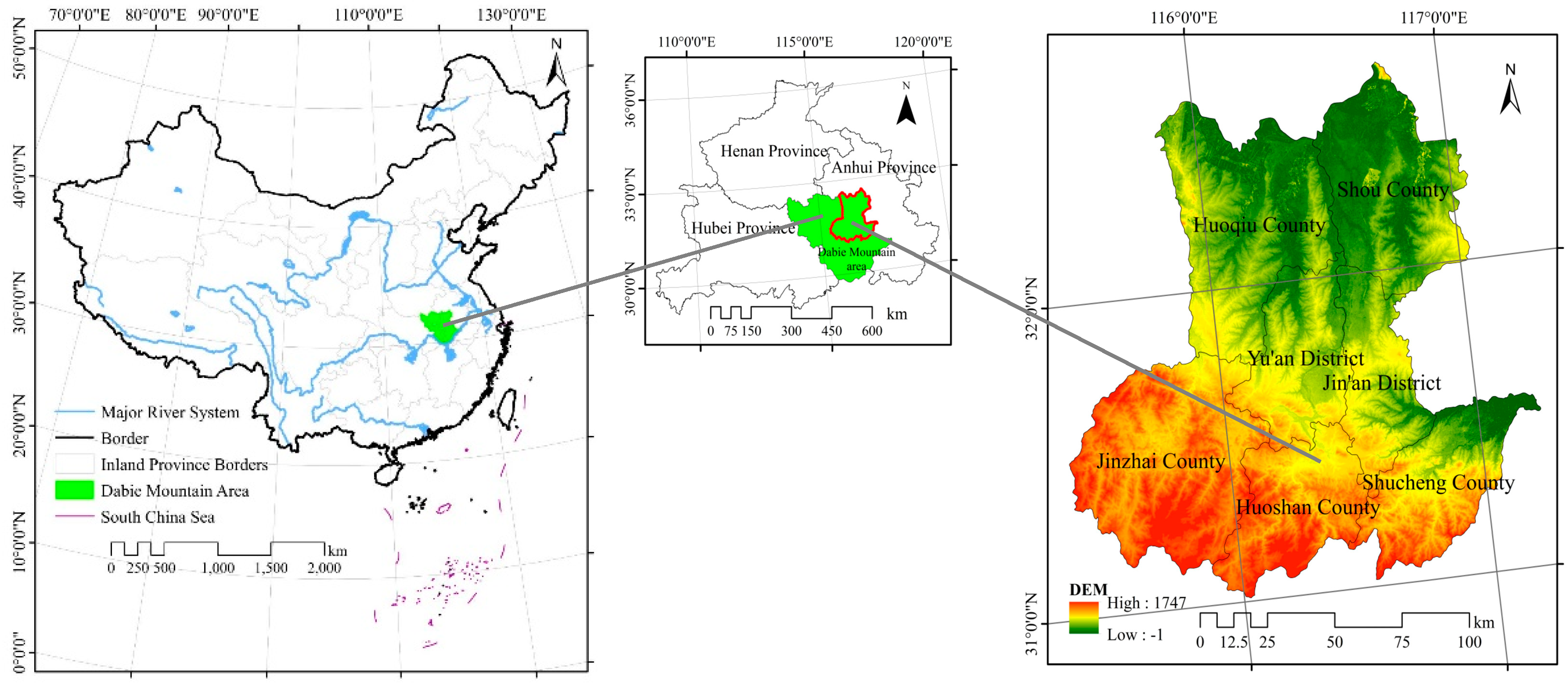
2.1. Study Area

The Dabie Mountains region (DBM) is located at the intersection of Hubei, Henan, and Anhui Provinces. This location is an important ecological function area in Central China and a significant ecological barrier in the middle and lower reaches of the Yangtze River [37,38]. The DBM of western Anhui Province is located in the northeast of the DBM region and the west of Anhui Province, China. It belongs to the core of the DBM, which is rich in tourism resources and is also one of the famous red scenic spots in China, as shown in Figure 1. The study area mainly includes five counties and two districts, namely Huoqiu County, Shou County, Jinzhai County, Huoshan County, Shucheng County, Yu’an District, and Jin’an District, covering 18,430 km², being dominated by middle and low mountains and hills, and belonging to the north subtropical warm and humid monsoon climate region. The annual average temperature ranges from 14–16 °C, the annual average rainfall from 1100–1450 mm, and the annual average sunshine hours from 2000–2200 h. The area is in the watershed of the Yangtze River and Huaihe River Basins in Anhui Province. Based on the Second National Remote Sensing Survey of Soil and Water Loss, ecological problems, such as soil and water loss in counties and districts, are prominent, making this a typical ecologically fragile area [39]. The DBM of western Anhui Province plays a core part of the key ecological function within the mountain range, and it is also the main water source for the Pishihang Irrigation area. As a famous reservoir region in China, it contains six large reservoirs, including Foziling, Mozitan, Bailianya, Meishan, Xianghongdian, and Longhekou, as well as the head water control project of the Pishihang Irrigation area [40].

2.2. Data Source and Processing

The types of data sources mainly included grid, vector, and text data in this study: land-use data with a spatial resolution of 30 × 30 m in 2005 and 2020, a digital elevation model (DEM) with a spatial resolution of 30 m, soil data in this study generated from a Chinese soil type distribution map and the Chinese soil dataset HWSD_ China_ Subset_ V1.1, precipitation of meteorological data in 2005 and 2020 collected from 44 meteorological stations in the study area and surrounding areas, annual actual evapotranspiration data from a geographic remote-sensing ecological network platform, normalized vegetation index (NDVI) data extracted from the remote sensing images (these were downloaded from geospatial data cloud website), and socioeconomic data mainly collected from relevant statistical yearbooks from 2006 to 2021. The descriptions of the data are shown in

Table 1. Description of data.

Category	Year	Data Type and Precision	Data Source
Land-use data	2005, 2020	Raster, 30 m	http://www.resdc.cn/ (acessesd on 11 February 2023)
DEM	2000	Raster, 30 m	http://www.resdc.cn/ (acessesd on 10 February 2023)
Soil data	2009	Vector, 1:106	http://www.resdc.cn/ (acessesd on 10 February 2023)
Precipitation	2005, 2020	Vector, point layer	http://www.resdc.cn/ (acessesd on 10 February 2023)
NDVI	2005, 2020	Raster, 30 m	http://www.gscloud.cn/ (acessesd on 15 January 2023)
Evapotranspiration data	2005, 2020	Raster, 30 m	http://www.gisrs.cn/ (acessesd on 6 January 2023)
Socioeconomic data	2006, 2021	/	statistical yearbooks

.

2.3. Methods

2.3.1. Ecosystem Service Evaluation

The five typical ESs and their formulas are shown below, including food supply, soil retention, water yield, carbon storage, and biodiversity maintenance in the list of ESs.

(a) Food supply (fs): Food supply service is an important service, in an agricultural ecosystem, which plays a vital role in human survival and regional development [41]. The type and quantity of food supply selected for this study were mainly derived from the food types and corresponding outputs provided in relevant statistical yearbooks. In terms of calculation methods, we allocated the output of grain according to the grid unit of cultivated land, the output of meat according to the grid unit of grassland, and the output of aquatic products according to the grid numbers of the water bodies. The specific methods were as follows. First, using conditional functions in ArcGIS, information on cultivated land, grassland, and water bodies were extracted from the land-use data of the study area. Second, for cultivated land and grassland, we allocated the outputs based on the ratio of the NDVI value of each grid to the total NDVI value of different land types, and ultimately allocate the outputs of grain, meat, and milk products to the cultivated land and grassland grid units, respectively [42]. For the allocation of aquatic products, we used an average allocation method based on the total number of water body pixels—that is, the ratio of the output of aquatic products to the total number of water grid cells—to evenly allocate the number of aquatic products. Finally, all land-use types were merged with the support of ArcGIS, resulting in a grid map of food supply services. The formula used for NDVI allocation is as follows:

$$G_i=G_{sum}\times \raisebox{1ex}{$NDV{I}_i$}\!\left/ \!\raisebox{-1ex}{$NDV{I}_{sum}$}\right.$$

(1)

where G_i is the output of grain, meat and milk products distributed by cell i, G_sum is the total output of grain, meat, and milk in the DBM of western Anhui Province, NDVI_i is the normalized vegetation index of cell i, and NDVI_sm is the sum of the NDVI values of cropland or grassland in the study area.

(b) Soil retention (sr): In this study, we used the sediment delivery ratio model, which is a submodel in the InVEST software, to estimate the amount of potential soil erosion (RKLS) and actual soil erosion (USLE) of each cell unit based on the Universal Soil Loss Equation (USLE), and then calculate the difference between these values to obtain soil conservation (SR) data. The formula used is as follows:

$$USLE=R\times K\times LS\times C\times P$$

(2)

$$RKLS=R\times K\times LS$$

(3)

$$SR=RKLS-USLE$$

(4)

where Sr is the amount of soil retention (t·hm⁻²·a⁻¹) and R is the rainfall erosivity (MJ·mm·hm⁻²·h⁻¹·a⁻¹). R was calculated based on the monthly average precipitation and annual average precipitation in the study area by using Wischmeier’s formula [43]. K is the soil erodibility (t·hm²·h·hm⁻²·MJ⁻¹·mm⁻¹), which was calculated by using the EPIC formula [44] on the basis of the relevant soil data, LS is the slope length gradient factor, which was extracted by the watershed slope length and slope factor calculation method [45] based on the DEM, P is the factor of water and soil conservation measures, which was determined by the slope index α [46], C is the vegetation coverage and crop management factor, which was calculated by the relationship formula between vegetation coverage and C value [47], and the value range is from 0 to 1.

(c) Water yield (wy): The water yield submodel in the InVEST software was applied to estimate the water yield. The water yield module in the InVEST model is mainly based on the Budyko curve and water balance principle [44]. The water yield capacity is equal to the precipitation on each grid in the study area minus the actual evapotranspiration (including soil evapotranspiration and plant evapotranspiration). Compared with other hydrological models, the InVEST model has advantages in the spatial expression and visualization of calculation results [48,49]. The formula is as follows:

$$Y\left(x\right)=\left(1-\raisebox{1ex}{$AE{T}_{\left(x\right)}$}\!\left/ \!\raisebox{-1ex}{$P_{\left(x\right)}$}\right.\right)\cdot P_{\left(x\right)}$$

(5)

where Y_(x) is the annual water yield (mm) at cell x, AET_(x) is the annual actual evapotranspiration (mm) at cell x, and P_(x) is the annual average precipitation (mm) at cell x.

(d) Carbon storage (cs): Carbon storage mainly includes four basic carbon pools: aboveground biomass, underground biomass, soil, and dead organic matter. The ES of carbon storage is to estimate the amount of carbon currently stored in the landscape on the basis of the average carbon density of carbon pools of different land-use types in the study area multiplied by the area of each land-use type [50,51]. In this study, the carbon storage module in the InVEST software was used to evaluate the amount of carbon currently in the study area. The formula is as follows:

$$C_{\_total}=C_{\_above}+C_{\_below}+C_{\_soil}+C_{\_dead}$$

(6)

where C_{_total} is the total carbon storage (t), C_{_above} is the carbon storage (t) of the aboveground biomass, C_{_below} is the carbon storage (t) of the belowground biomass, C_{_soil} refers to the carbon storage in soil, and C_{_dead} refers to the dead organic carbon storage.

(e) Biodiversity maintenance (bd): The InVEST software calculates habitat quality by combining landscape sensitivity and external threat intensity and evaluates biodiversity service function based on habitat quality [52]. The Habitat Quality module in InVEST was applied to evaluate the habitat quality index to reflect the function of providing biodiversity services (the InVEST model assumes that areas with good habitat quality have high biodiversity). The habitat quality index is a dimensionless comprehensive index to reflect the habitat suitability and habitat degradation degree of different land-use types in the study area. The calculation formula and model parameter table of the habitat quality index were derived from relevant references [44,53,54,55].

2.3.2. Spatial Expression and Measure of Trade-Offs and Synergies among ESs

(a) Expression of spatial heterogeneity for typical ESs: For better comparison and calculation in the next step, those five aforementioned ESs were standardized primarily to eliminate this dimension. In this paper, the Fuzzy membership method, which is mainly based on the overlay toolset of the spatial analysis toolbox in the ArcGIS 10.2 software, was used to normalize five typical ESs in the study area. After making them dimensionless, the Raster Calculator tool was used to overlay the normalized grid map of ESs to obtain the grid map of the total value of ESs in the study area. The amounts of change in ESs from 2005 to 2020 were obtained by calculating the differences between the ESs in 2005 and 2020. In addition, the Zonal Statistics function in ArcGIS was used to calculate the amounts of the five ESs in the different administrative units, and then the characteristics of spatial distribution and spatial heterogeneity of the total value, and the amounts of change in ESs were discussed by calculating the local autocorrelation, i.e., the Moran’s I index, among ESs and drawing the map of local indicators of spatial association (LISA) based on GeoDA 10.0.

(b) Measure of trade-offs/synergies among ESs: The trade-offs and synergies among the five ESs were explored by using the spatial analysis tools in ArcGIS and the correlation analysis function in the R language software. First, random points were created by using the Create Random Points tool in ArcGIS to take raster values from the supply maps of various ESs to these points. Second, the attribute data of random points with the values of the ESs were imported into the Excel software. Finally, the data were imported into the R language, and the maps of the lower triangle and the maps of correlation heat with the coefficient matrix were produced based on the R language, which can measure the trade-offs/synergies among the five ESs.

(c) Spatial patterns of trade-offs/synergies between ESs pairs and identification of ES bundles: In this study, we aimed to provide a clearer visualization of the spatial distribution characteristics of the trade-offs/synergies between ESs pairs. First, the mean values of ESs at the township administrative scale were computed using the Zonal Statistics function in ArcGIS 10.2. Then, we used the bivariate global and local Moran’s I indices to further explore the spatial expression of trade-offs/synergies between ESs pairs [49]. Second, to classify the homogeneity of ESs, ecosystem service bundles at the scale of township administrative units were identified by using the SOM method. The SOM method changes the network parameters and structure in a self-organizing and adaptive manner by automatically finding the intrinsic laws and essential properties in samples. It is an unsupervised learning neural network method that can allocate each township administrative unit into ecosystem service bundles based on the similarities of ecosystem service co-occurrence in space [56]. In this study, the identification of ES bundles, by using the SOM method, was executed in the R language.

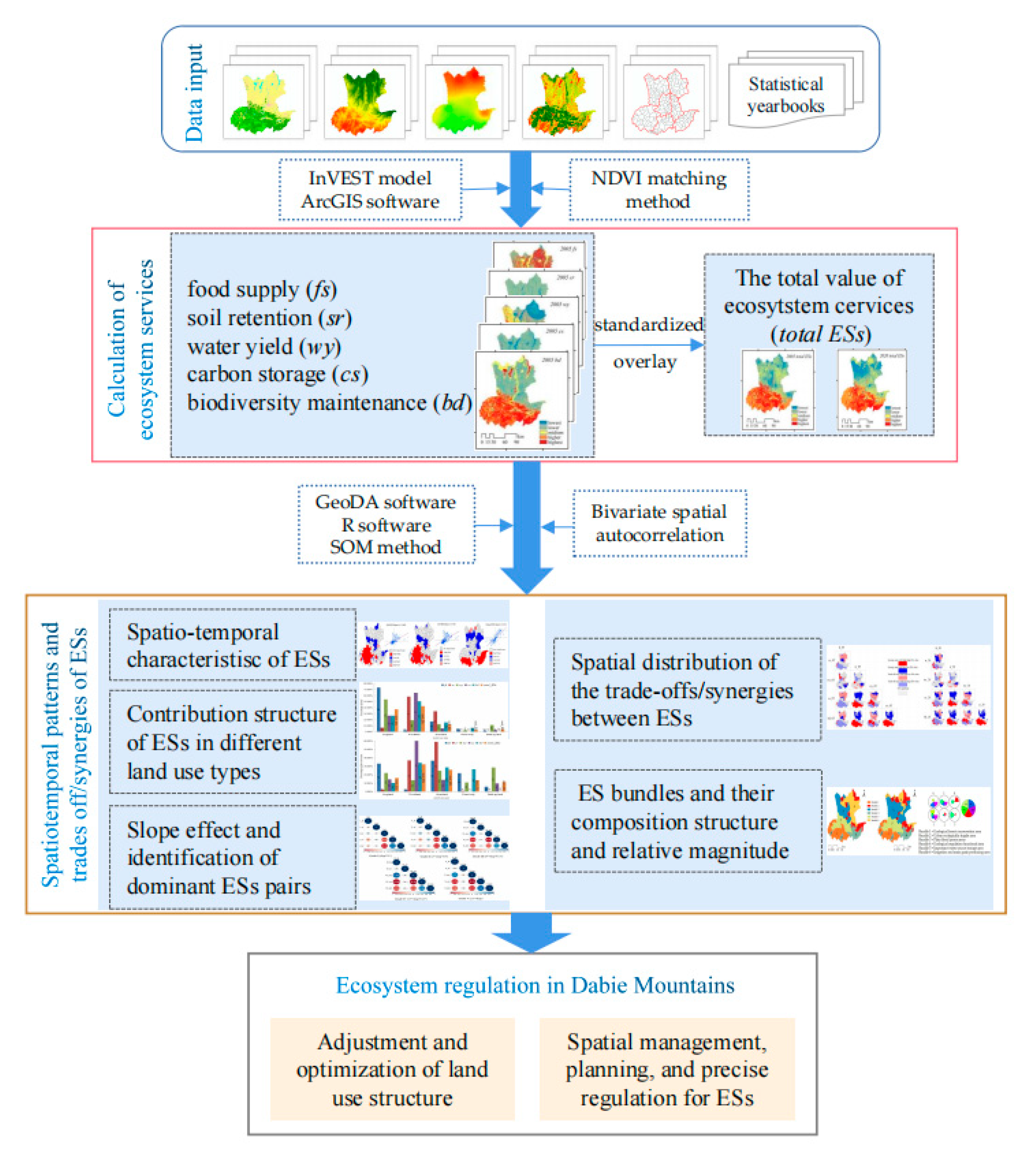
2.3.3. The Research Framework

In the study, the correlation coefficient method, exploratory spatial data analysis (ESDA), bivariate spatial autocorrelation, SOM and InVEST models, R software, ArcGIS software, and GeoDA software were applied. First, we evaluated ESs from 2005 to 2020 and analyzed their spatiotemporal patterns. Second, ecosystem service contribution structures in different land-use types, the slope effect, and trade-offs/synergies correlations between ESs were analyzed. Last, the spatial expressions of trade-off/synergy relationships between ESs pairs, ecosystem service bundles, and spatial distribution and composition structures of ecosystem service bundles were identified and analyzed. The utilized research framework is shown in Figure 2.

3. Results

3.1. Spatiotemporal Variation of ESs

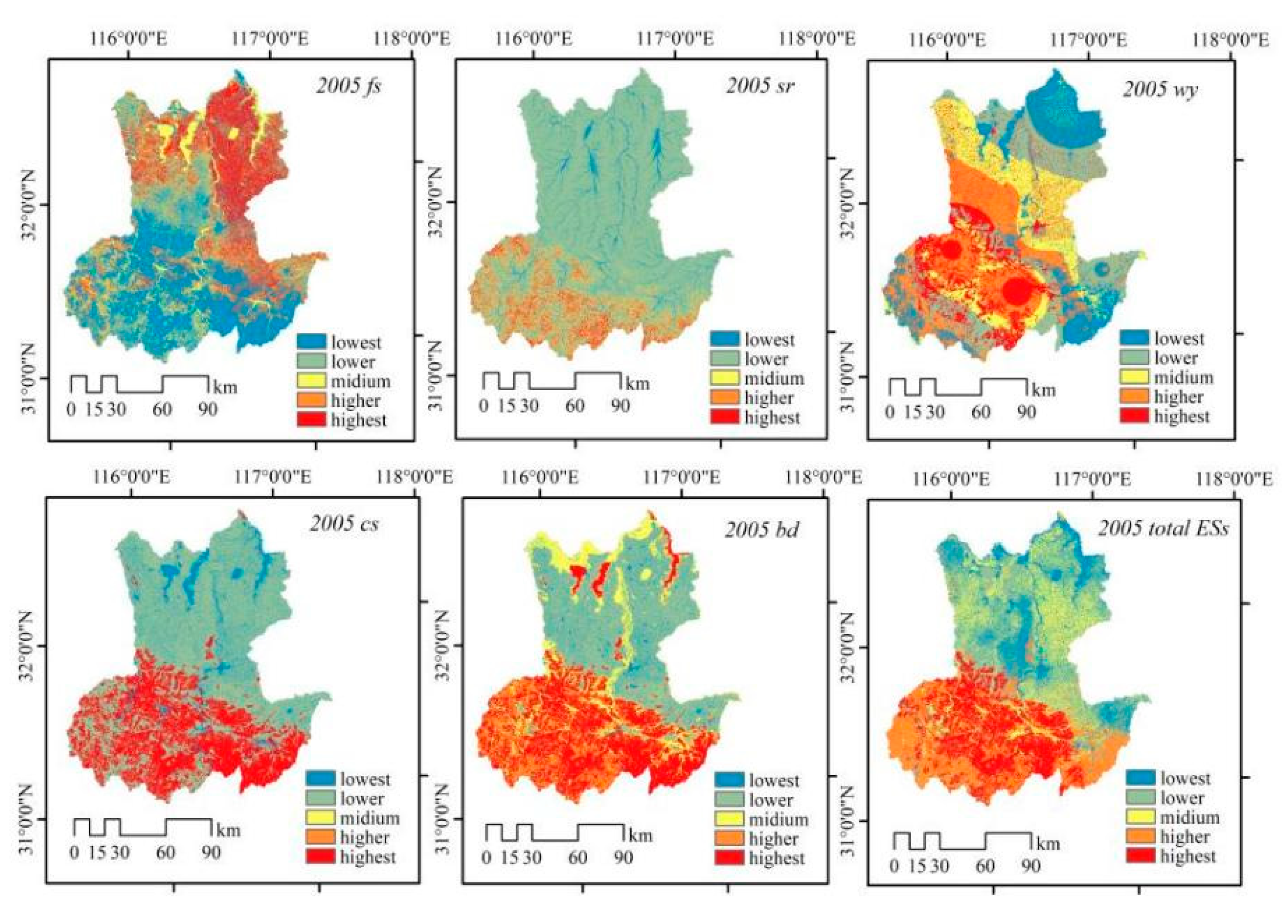
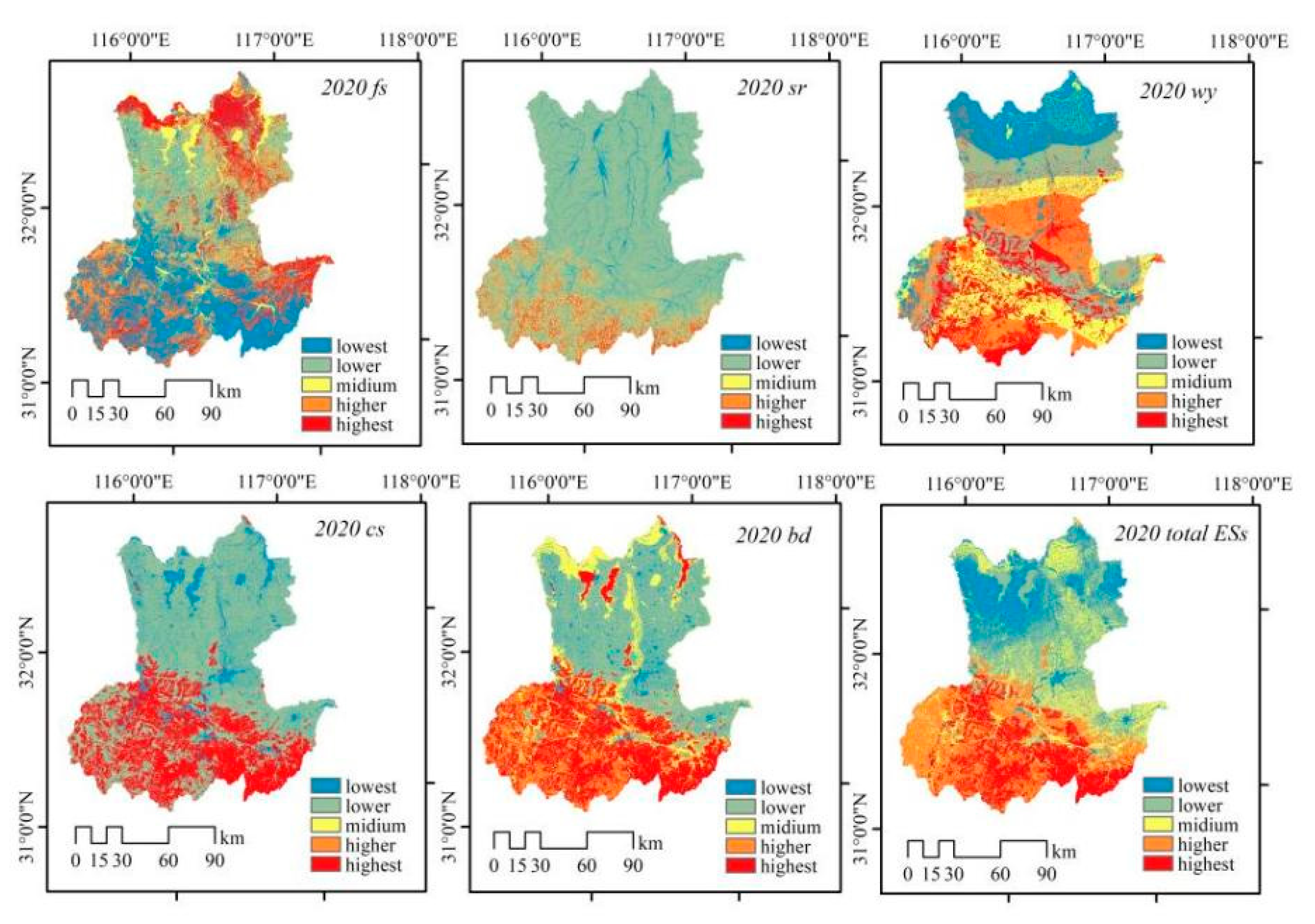
3.1.1. Spatial Patterns and ESs Changes

The five ESs, i.e., food supply, soil retention, water yield, carbon storage, and biodiversity maintenance, were standardized after the assessment and then were classified into five levels in the ArcGIS software, forming the lowest, lower, medium, higher, and highest levels, respectively. The total ESs in the DBM of western Anhui Province showed a changing trend of “three increases and two decreases.” Among the five ESs, food supply, soil retention, and water yield had increased, with annual growth rates of 2.83%, 6.50% and 2.99%, respectively from 2005 to 2020. Conversely, the other two ESs, carbon storage and biodiversity maintenance, had decreased with annual decline rates of 0.03%, and 0.07%, respectively, showing weak downward trends from 2005 to 2020. Since the DBM was situated in the national rainfall center in 2020, water yield increased from 682.22 mm in 2005 to 987.67 mm in 2020, with a growth of 44.77%. Meanwhile, soil conservation changed fastest, rising from 1.74 × 10⁸ t in 2005 up to 3.44 × 10⁸ t in 2020, with a growth of 97.49%; food supply also showed an upward trend, from 664.07 × 10⁴ t in 2005 up to 945.67 × 10⁴ t in 2020, with a growth of 42.41%.

Spatially, the low-level region of food supply was mainly distributed in the southern parts of the study area, such as Jinzhai County, Huoshan County, and the south of Shucheng County. The reason for this is that the southern mountainous areas are mainly forest land and slope farmland, and hence the food supply is low, whereas the high-level food supply region was mainly distributed in the northern parts of the study area, such as Huoqiu County and Shou County. It must be specially noted that Shou County is a major grain-producing county in China. This region has excellent irrigation water quality, moderately fertile soil, and a fine climate condition; hence, the region’s food supply capacity is the highest in the study area. The statistical description of food supply also showed that the maximum, mean, and variance of food supply on the cell unit had increased, indicating that the measures of cropland consolidation in the DBM of western Anhui Province had played a certain role in promoting grain production, and that the measures of cropland concentration and large-scale management had optimized the spatial layout of food supply carriers and then improved the food supply. The areas with high levels of water yield were found to be distributed in the south of the study area, whereas the low-level areas were in the north of the study area; the reasons for this are mainly related to the heavy rainfall and relatively low evaporation [57] in the southern mountainous areas (Figure 3 and Figure 4).

From the perspective of spatial patterns, the spatial characteristics of ESs were obvious. The low-level region of soil retention was mainly located in the middle and north of the study area. The high-level region of soil retention was mainly distributed in the south of the study area. This area is the intersection of nature reserves, scenic spots, and forest parks. Thus, here, the regional vegetation coverage is high, and the soil retention is relatively high. The high-level region of carbon storage was mainly located in the southern mountainous area, which has a humid climate, high vegetation coverage, and high soil organic matter content, whereas the vegetation coverage and soil organic matter content in the northern area are relatively low due to the presence of cropland and built-up land. Therefore, the carbon storage in the northern parts was generally lower than that in the south of the study area. The high-level region of biodiversity maintenance was mainly distributed in the south of the study area, whereas the low-level region was mainly located in the scope of built-up land with a low density of vegetation coverage and strong interference of human activities.

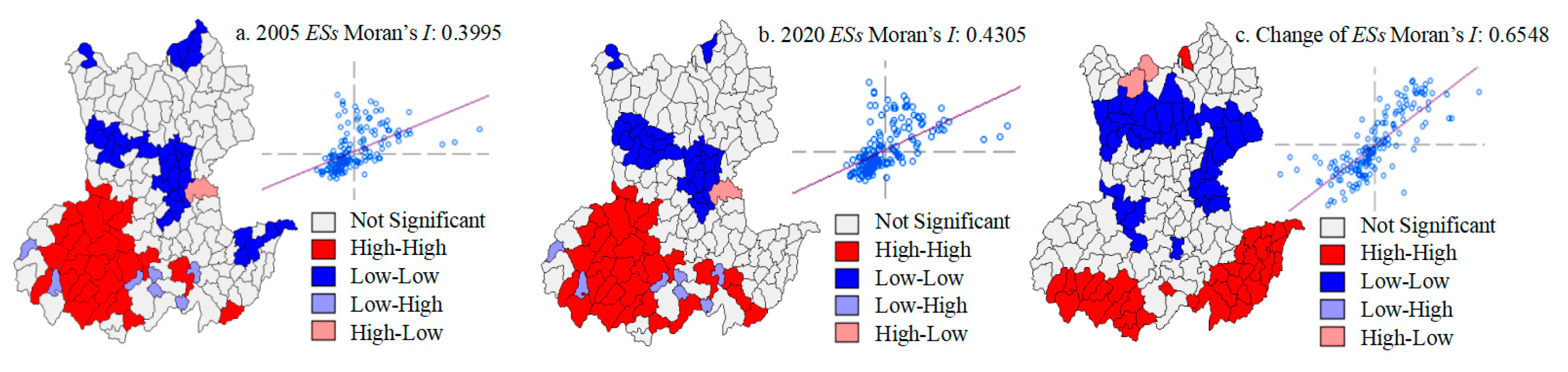
3.1.2. Spatiotemporal Heterogeneity of ESs

Revealing the spatial clustering characteristics of the total ESs and the temporal change of ESs in the study area will help us understand the spatial heterogeneity of ESs and perform effective regulation for ESs in practice. In this study, ArcGIS was used to derive spatial statistics on the total ESs in 2005 and 2020 and the temporal change of ESs from 2005 to 2020 according to township units, then local spatial autocorrelation analysis was carried out. The Moran’s I index and the map of local indicators of spatial association (LISA) were generated, as shown in Figure 5 by using the GeoDA software. The total of ESs in 2005 and 2020 and the change amounts of ESs from 2005 to 2020 in the DBM of western Anhui Province had reasonably significant spatial heterogeneity.

The results showed that the Moran’s I indices of the total ESs in 2005 and 2020 were 0.3995 and 0.4305 with Z-Score over 2.58, respectively, indicating that they passed the significance test at the 0.01 level and the spatial clustering effect was highly significant. The map of LISA shows that the scope of High-High clustering and Low-Low clustering area in 2005 and 2020 were also mainly located in the central north and the south of the study area, respectively. Overall, the spatial distribution of the total ESs had still changed in the past 15 years. The number of units in the High-High region increased from 27 in 2005 to 29 in 2020, and the number of units in the Low-Low region decreased from 31 in 2005 to 23 in 2020. The number change areas are mainly located in the north and southeast of the study area (Figure 5). For further research on the spatial characteristics of the temporal changes of ESs, the differences between the total ESs of each township unit in 2005 and in 2020 were calculated based on the ArcGIS software, and then the changing trend and its spatial heterogeneity in the township unit were analyzed by using the GeoDA software.

From 2005 to 2020, there existed 58 township units with an upward trend in the amount of ESs, and these were mainly distributed in the south and north of the study area. Among them, there existed 20 units in Shucheng County, 12 units in Jinzhai County, and 9 units in Huoshan County. The total number of these units accounted for 70.69% of the total number of units, with a rising trend of ESs. Contrarily, there existed 64 township units with downward trends of change, and these were mainly distributed in most townships of Yu’an District and Jin’an District in the middle and north of the study area, the south of Huoqiu County and Shou County, and the north of Jinzhai County and Huoshan County; of these over 80% were located in Yu’an District, Jin’an District, Huoqiu County, and Shou County, and the spatial distribution here formed a basin structure of “low, middle and high outside”. The local autocorrelation analysis showed that the Moran’s I index of the ecosystem service change was 0.6548; meanwhile, the Z-score was greater than 2.58, indicating that the spatial correlation had reached a highly significant level. The LISA cluster map showed that the Low-Low area of the ecosystem service change was mainly distributed in Huoqiu County, Shou County, and Jin’an District in the middle and north of the study area, with a total of 38 township units, whereas the High-High region was mainly located in Jinzhai County and Shucheng County in the south of the study area, with a total of 36 township units (Figure 5). Local spatial autocorrelation analysis accurately expressed the clustering characteristic of temporal change of ESs from 2005 to 2020 in the study area, and this can provide a decision-making basis for township ecological planning and ecosystem function regulation to some extent.

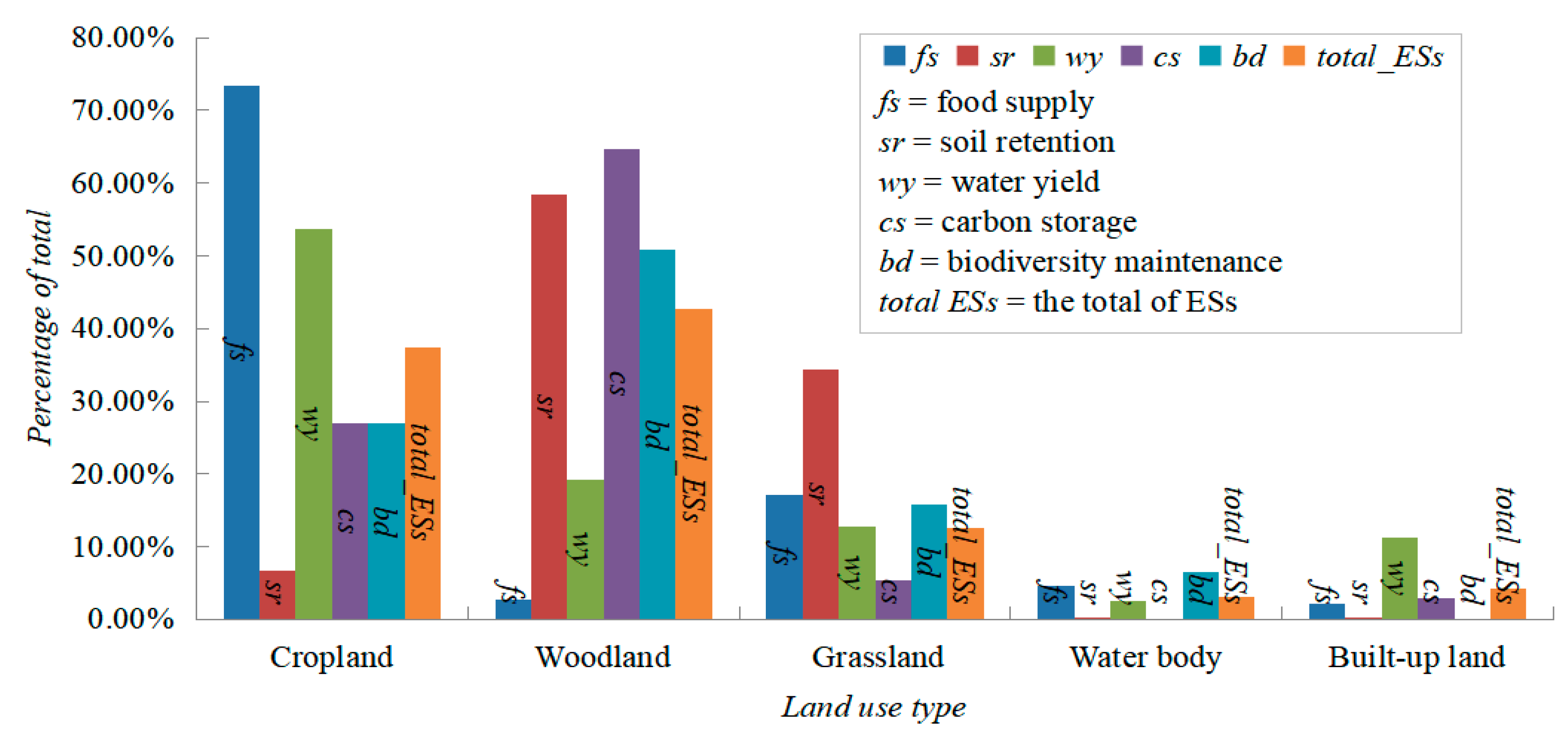
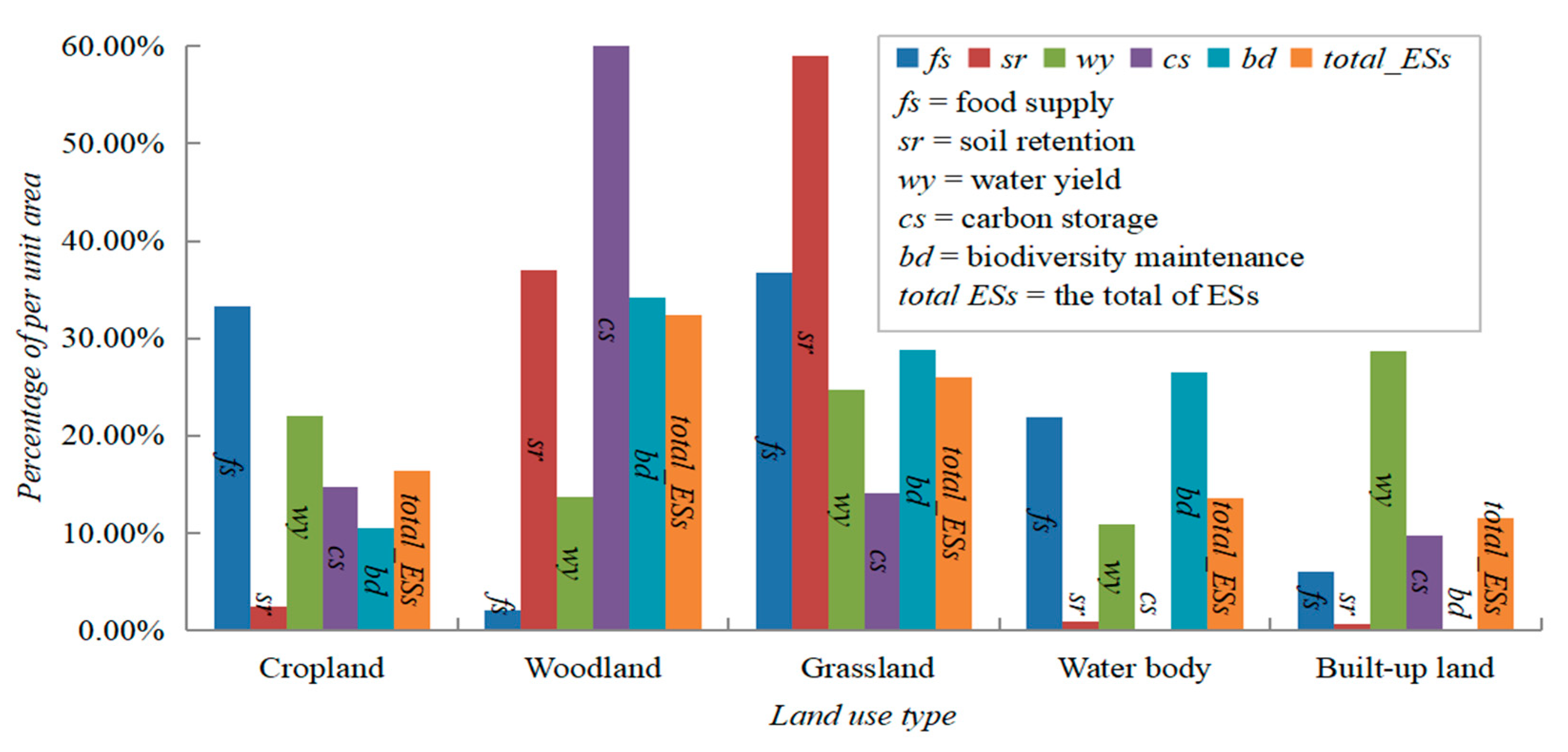
3.2. Impact of Land-Use Types on the Supply of ESs

Land use/cover change is an important reason for the spatial differences between surface ESs. Different land-use types affect ESs distinctly [58]. In this study, the Condition Analysis Function in the ArcGIS software was used to extract the cells of cropland, woodland, grassland, water bodies, and built-up land, and then the cells of the five ESs in the study area were extracted in accordance with the positions of cells in different land-use types.

Taking 2020 as an example, the results showed that the amounts of ESs from cropland and woodland accounted for 37.42% and 42.70% of the total ESs in the DBM of western Anhui Province, respectively. Therefore, cropland and woodland were the main contributors to the total ESs in the study area, whereas water bodies accounted for only 3.01% of the total ESs in the study area because of their relatively small area proportion of the study area. In terms of the composition of each ecosystem service, the sources of ESs were found to be significantly different, as can be seen in Figure 6. (a) The total food supply mainly came from cropland, accounting for 73.41%. (b) The total of soil retention mainly came from woodland and grassland, accounting for 58.44% and 34.29%, respectively. (c) The total of water yields mainly came from cropland, woodland, and grassland, accounting for 53.75%, 19.22%, and 12.81%, respectively. (d) The total of carbon storage mainly came from cropland and woodland, accounting for 26.91% and 64.77%, respectively. (e) Similarly, over 80% of the total biodiversity maintenance came from cropland and woodland. These results show that the supply sources of ESs in the study area were mainly cropland and woodland, whether with regards to the composition of total ESs or the composition of single ESs, as shown in Figure 6.

From the area proportion of various land-use types, it is clear that the proportion of cropland accounted for 48.89% of the total area in 2020, making it the largest land-use type in the study area. The woodland area accounted for approximately 28.16%, the grassland area accounted for roughly 10.38%, the total area of built-up land accounted for about 7.84%, whereas the total area of water bodies accounted for only 4.72%, making this the smallest land-use type in the study area. The area proportion of the five land-use types in the study area was significantly different. Therefore, further analysis of the composition of ESs per unit area can reflect the supply capacity of different land-use types to the total of ESs in the study area. The results showed that in terms of supply capacity per unit area, the main contribution to the total ESs in the study area in 2020 was woodland and grassland, accounting for 32.42% and 26.01%, respectively, which can be seen in Figure 7.

Based on the composition of each ecosystem service per unit area, the following were evident: cropland and grassland contributed over 70% to food supply per unit area; soil retention per unit area mainly came from woodland and grassland, accounting for 37.04% and 58.96%, respectively; built-up land was the main source of water yield per unit area, accounting for 28.66%; carbon storage per unit area mainly came from woodland, accounting for 61.47%; and woodland, grassland, and water bodies had strong supply capacities of biodiversity maintenance per unit area, accounting for 34.21%, 28.79%, and 26.57%, respectively (Figure 7). The results revealed that in view of the supply composition of the total amount of ESs and the supply capacity per unit area comprehensively, the ESs in the study area mainly came from the woodland, which accounts for 42.70% of the total amount of ESs in the study area and 32.42% of the ESs per unit area. Therefore, the contribution of the land-use type of woodland to ESs in the DBM of western Anhui Province reached approximately 1/3.

3.3. Trade-Offs and Synergies among ESs

3.3.1. Impact of Slope on Trade-Offs and Synergies among ESs

The terrain is an important factor affecting land use, ecosystem, and soil erosion. It controls the redistribution of surface water, heat, and other energies, and dominates the intensity and direction of surface runoff [39]. Revealing the influencing mechanism of slope on trade-offs and synergies among ecosystem services is helpful to establish multi-scale ecosystem function regulation and ecological optimization decision-making schemes [36]. Therefore, the effects of slope on trade-offs and synergies among ESs, based on the correlation analysis functions in the R language, were discussed in the study. In this study, the study area was reclassified into five grades based on slope, namely, Grade I slope area (slop1 ≤ 2°), Grade II slope area (2° < slop2 ≤ 6°), Grade III slope area (6° < slop3 ≤ 15°), Grade IV slope area (15° < slop3 ≤ 25°), and Grade V Slope area (25° < slop5) according to the technical specification for land-use status investigation by using the ArcGIS software.

Taking 2020 as an example, random points were created within the scope of different grades; then, the attribute values of the five ESs were extracted at the corresponding random points, and then the attribute values were imported into the R language to generate the maps of the lower triangle, and finally, the correlations between ESs pairs were analyzed on the basis of the maps. In a map of the lower triangle, the red round cake indicates the trade-offs with negative correlations between these pairs of ESs, and the blue round cake indicates synergies with positive correlations. The darker the color and the larger the round cake, the greater the correlation coefficient and the more significant the trade-offs and synergies between ESs. The results show that different trade-offs and synergies were found among ESs in the study area based on the different slope grades, and the numbers of trade-offs were more than those of synergies on the whole. The trade-offs and synergies among ESs had different sensitivities to the slope grade changes, i.e., trade-offs between wy and bd, wy and cs were always found under five slope grades. As we can see in Figure 7, the correlation coefficients of the trade-offs between wy and bd in five slope conditions were −0.78, −0.75, −0.62, −0.65 and −0.73, respectively, while the correlation coefficients of the trade-offs between wy and cs in five slope conditions were −0.65, −0.72, −0.83, −0.89 and −0.89, respectively, with all correlation coefficients reaching significant levels, and the trade-offs became increasingly significant with increase in slope grade. Similarly, weak synergies were found between fs and wy at the slope Grade I (slop ≤ 2°) and II (2° < slop ≤ 6°), and the synergies became more significant at the slope Grades III (6° < slop ≤ 15°), IV (15° < slop ≤ 25°), and V (25° < slop), which reveal a typical slope effect. Conversely, bd and cs always showed significant synergies at different grades of slope. As we can see in Figure 8, the correlation coefficients of the synergistic relationships between bd and cs in five slope conditions were 0.76, 0.80, 0.66, 0.69 and 0.80, respectively. The relationships between fs and sr, sr and wy, sr and bd, and sr and cs at Grades III (6° < slop ≤ 15°), IV (15° < slop ≤ 25°), and V (25° < slop) were unclear because their correlation coefficients were small, despite the fact that there were some trade-offs and synergies with weak correlation below the slop Grade II.

The results unveiled that when the slope increased, the correlation coefficients between most ESs increased gradually: that is, the significance of trade-offs and synergies increased with slope increase, such as the pair of ESs between wy and cs, and between cs and bd. Conversely, there remained a few correlations between ESs that were less sensitive to slope change, such as these pairs: fs and sr, wy and sr, cs and sr, and cs and bd. Ultimately, the slope effects on trade-offs and synergies were significant between typical ecosystem service pairs in the study area (Figure 8). The diversity of ESs and the identification of trade-offs and synergies at different slope levels in the study area can provide a practical decision-making basis for ecological management. For example, on a slope greater than 25 degrees, we found that the trade-off relationship between carbon storage and water yield reached the maximum and the synergies between carbon storage and biodiversity maintenance also reached the maximum. Therefore, the planning of ES demand in areas with complex terrain must be more cautious than the planning in flat areas, and thereby, based on the corresponding trade-offs and synergies, a management and regulation strategy for maximizing ES supply in the study area can be proposed. However, the influencing mechanism of the slope effect on the trade-off/synergy changes among ESs warrants further analysis.

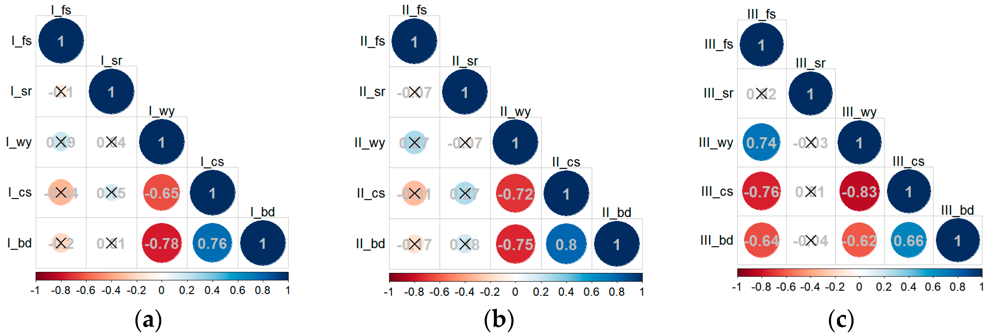
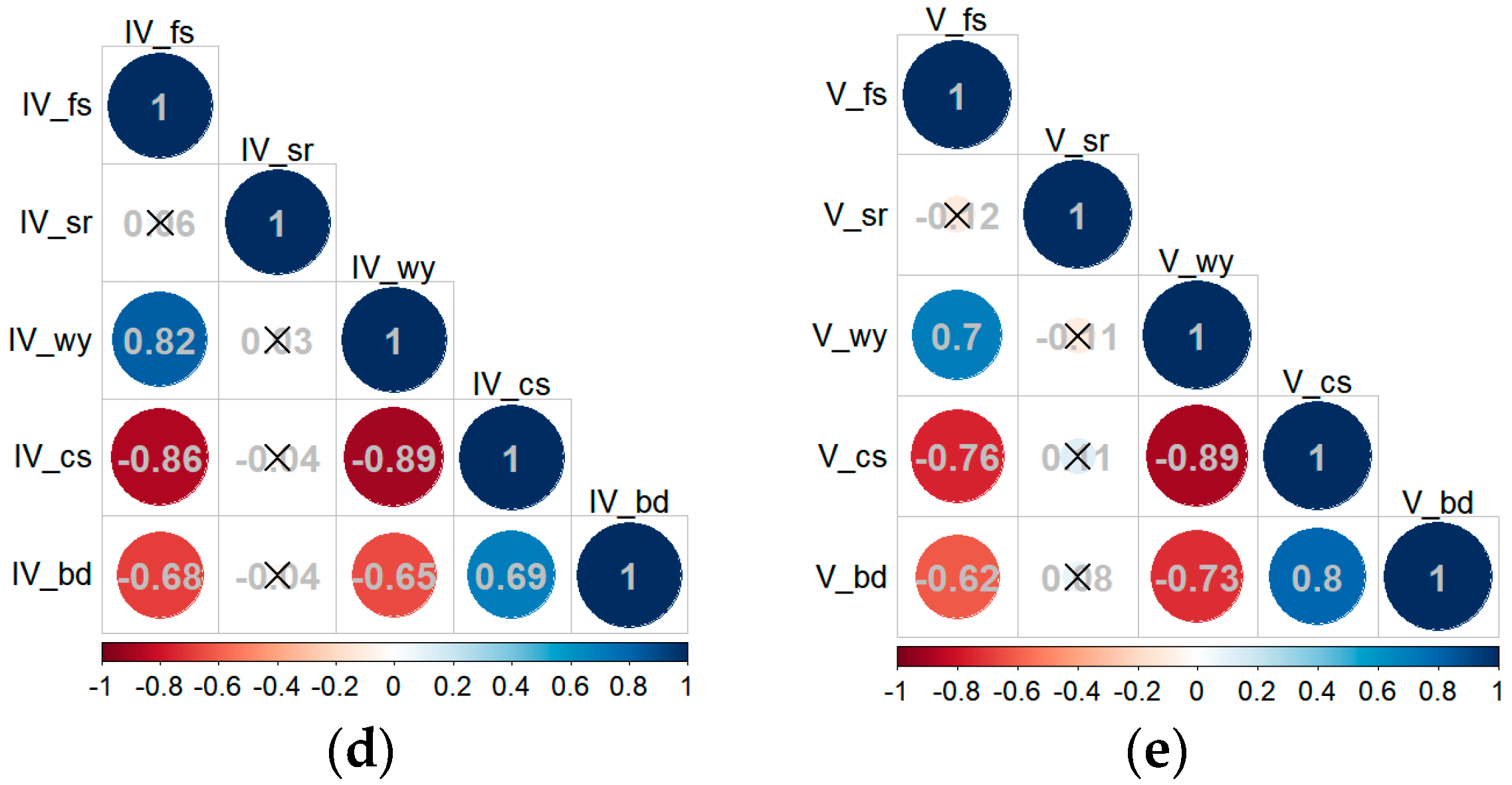
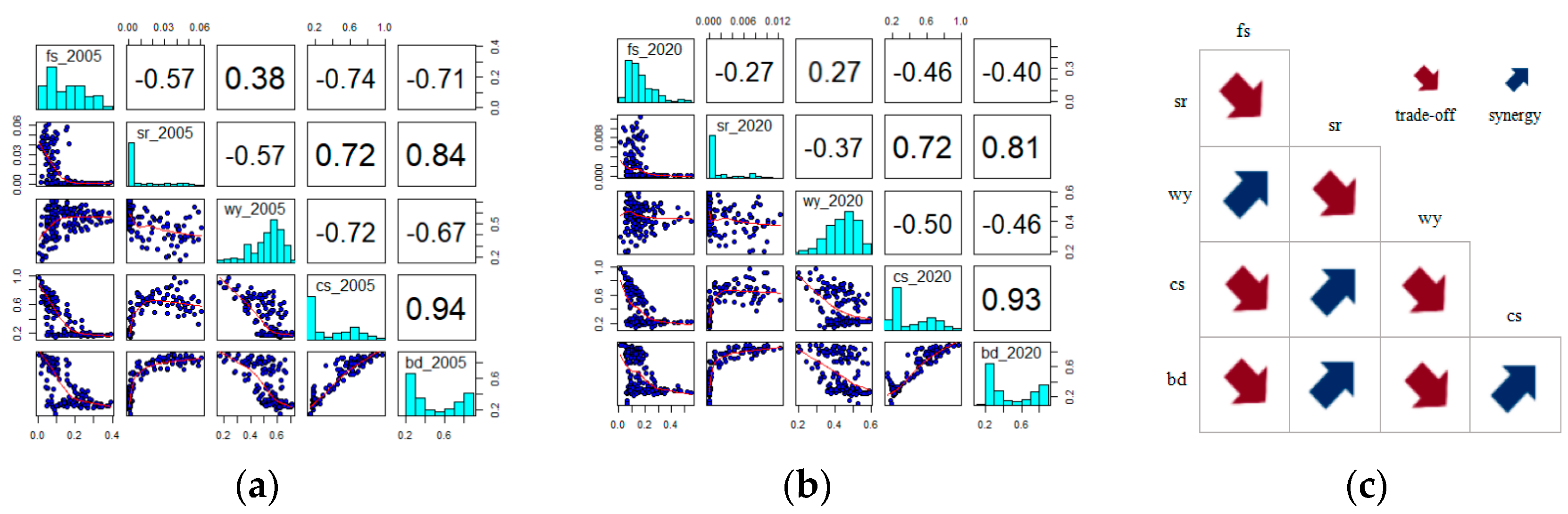
3.3.2. Temporal Characteristics of Trade-Offs/Synergies among ESs

Research on the temporal characteristics of trade-offs/synergies is beneficial to understand the law of mutual conservation between ESs to some extent. Based on the R language, correlation heat maps were generated in this study. In a scatter matrix of correlation heat maps, the histogram and kernel density curve of five services are on the main diagonal. The histogram can reflect the distribution characteristics of horizontal axis data (ESs), and the kernel density curve reflects the concentration degree of horizontal axis data distribution. The part above the main diagonal is the correlation coefficient between ESs. The part below the main diagonal is the scatter diagram and smooth-fitting curve between ESs.

The results uncovered that the correlation coefficients between these pairs of ESs in 2005 and 2020 mostly reached significance at the 0.01 level except for these pairs of ESs between fs and sr, and fs and wy, in 2020. Synergies with positive correlation were found between sr and cs, sr and bd, and cs and bd in 2005 and 2020. Among them, the positive coefficients between cs and bd reached above 0.90 in the two periods, and the correlation between these two was the strongest. Therefore, the relationship between cs and bd was identified as the dominant synergy in the study area. In comparison, these pairs of ESs, i.e., wy and cs, wy and bd, fs and cs, fs and bd, sr and wy, and fs and sr, showed the relationships of trade-offs with negative coefficients, of which the pair of ESs including wy and cs had the strong negative correlation, changing from −0.72 in 2005 to −0.50 in 2020; this was identified as the dominant trade-off relationship in the study area (Figure 9). In addition, in recent 15 years, the number of trade-off types and synergy types in the study area had remained unchanged. Among them, the type of synergies still accounted for 40%, and the type of trade-offs accounted for 60%, but the trade-off and synergy relationships between all pairs of ESs were weakening. Among them, the maximum value of the correlation coefficient of the trade-off relationship decreased from 0.72 in 2005 to 0.50 in 2020, showing an obvious weakening trend, and yet the correlation coefficient of the synergetic relationship showed a weak downward trend as a whole. Ultimately, the wy and cs and cs and bd were the dominant relationships of trade-offs/synergies among different ESs in the study area. Revealing the temporal characteristics and the dominant trade-offs and synergies is theoretically and practically valuable for ecosystem function optimization and ecological restoration in the DBM of western Anhui Province. Further research on trade-offs and synergies under the conditions of the fine terrain and long time series can effectively reveal the changing characteristics and driving mechanisms of various ESs.

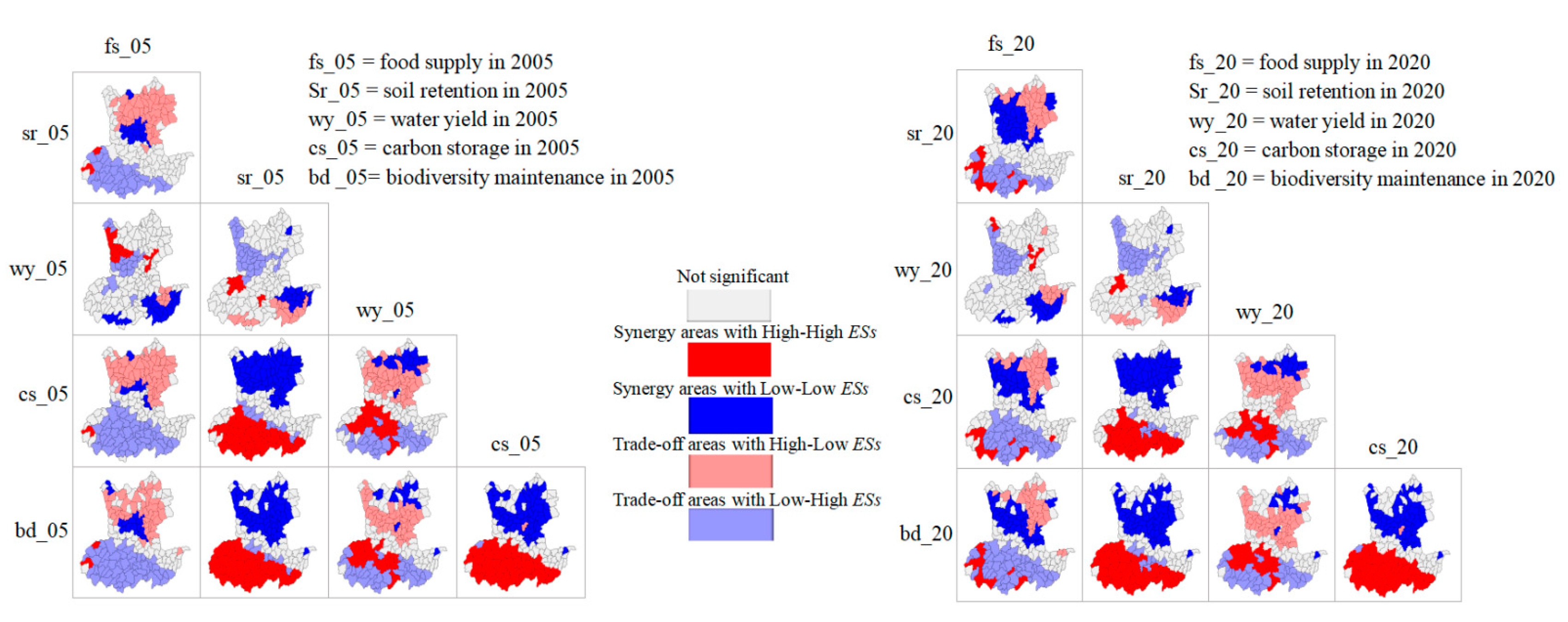
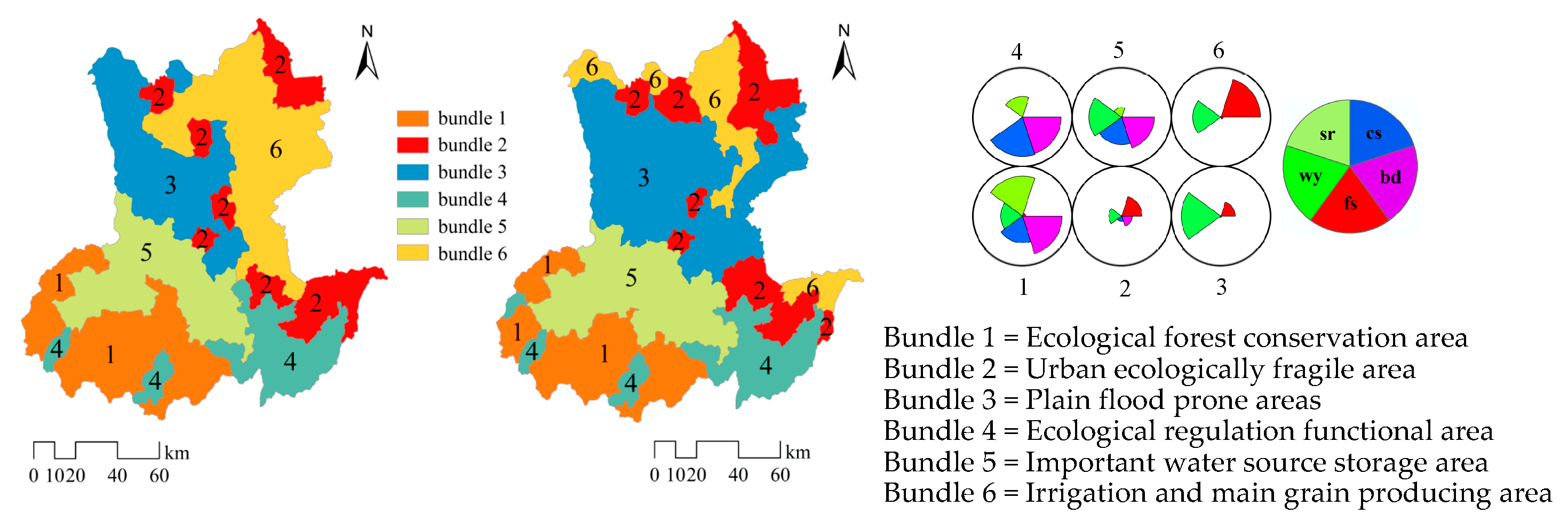
3.3.3. Spatial Distributions of Trade-Offs/Synergies between ESs Pairs

The study of trade-off/synergy relationships based on quantitative methods of correlation coefficients can easily and conveniently identify the types of trade-offs and synergies in the interrelationships between typical ESs in the DBM of western Anhui Province, as well as identify the strengths and weaknesses of correlations between pairs of ESs. Although the correlation coefficient matrix can be used to quickly identify trade-off/synergy relationships between two pairs of ESs, it is weak in expressing the spatial distributions of the trade-off/synergy effects between ESs specifically. Therefore, strengthening the spatial expression of trade-off/synergy relationships between ESs is beneficial for the precise regulation of ecosystems.

This study analyzes the spatial patterns of trade-offs and synergies of ESs based on the bivariate local Moran’s I. Figure 10 shows that the spatial patterns of trade-offs and synergies between different ecosystem service pairs differed significantly, with the High-High and Low-Low values of the bivariate local Moran’s I expressing the High-value and Low-value areas of synergies between ESs, respectively, and the High-Low- and Low-High -value areas of Moran’s I expressing trade-offs between ESs, respectively. The results showed that the spatial distribution pattern of trade-off/synergy relationships among ESs in the study area had not changed much in the past 15 years, and presented a more stable spatial pattern. This was strongly related to the progress of conservation and development in the DBM as well as land-use changes and the level of socio-economic development in the region. In the years 2005 and 2020, sr and cs, sr and bd, and cs and bd showed synergistic relationships in many places spatially, in which the High-value synergistic areas were distributed in the south of the study area, while the Low-value synergistic areas were mainly located in the north-central part of the study area, showing significant spatial differences.

Bivariate local spatial autocorrelation clearly reveals the spatial trade-off/synergy relationships of ecosystem services, but ignores potential patterns of spatial association of ESs and does not provide insight into the interdependence between multiple ESs [59]. A bundle of ESs is a group of ESs that recur in time and space, reflecting the interdependence of those ESs [30]. SOM is an unsupervised learning neural network method that measures the similarity between ESs of different township units based on the similarity principle, and classifies township units with high similarity into the same ES bundles. In this study, the SOM method was applied to identify ES bundles and their spatial distribution at the township scale, and the results of SOM self-organizational mapping analysis can be used to tailored management measures and solutions for different ecological environments.

The SOM cluster analysis of five typical ESs in the DBM of western Anhui Province finally identified six types of ecosystem service bundles. Based on their clustering characteristics and combined with the realities of the study area, these six types of ecosystem service bundles were named ‘ecological forest conservation areas’, ‘urban ecologically fragile areas’, ‘plain flood prone areas’, ‘ecological regulating functional areas’, ‘important water reservoir area’, and ‘irrigation and main grain production areas’ in this study (Figure 11). In terms of area comparison, in 2005, the areas of ecosystem service bundles 1~6 were 3495.82 km², 2364.96 km², 3249.93 km², 2130.38 km², 2997.73 km², and 4192.05 km², respectively; in 2020, the areas of ecosystem service bundles 1–6 were 2955.69 km², 2643.15 km² 5475.06 km², 2058.80 km², 3348.84 km², and 1949.36 km², respectively. The transition of different bundles at the township administrative scale revealed that the areas of Bundle 2, Bundle 3, and Bundle 5 expanded whereas the areas of Bundle 1, Bundle 4, and Bundle 6 shrank from 2005 to 2020 in the study area. Different service bundle areas have formed corresponding ecological function areas, which are important for the ecological regulation of the DBM.

As shown in Figure 11, bundles of similar ESs are obviously clustered in space, while the composition structure of each ecosystem service bundle has obvious differences, and the rose diagram in this paper shows the relative size of each ecosystem service in each ecological subdistrict of the DBM of western Anhui Province. In Bundle 1, the composition structure of ESs is relatively balanced, and the supply of ESs is high, mainly including sr, bd, cs, and wy, and this type of service is mainly located in the southern forest area with high topography, so it is named ‘ecological forest conservation areas’. In Bundle 2, the amount of ESs is scarce, and these types of service are mainly located in the area of urban construction land, so the bundle is named ‘urban ecological fragile areas’. In Bundle 3, the ecosystem service type is mainly wy, and the area is mainly located in the north-central part of the relatively gentle topography, so it is named ‘plain flood prone areas’. Bundle 4 is mainly located in the mountainous area in the south of the study area, and the ecosystem service types are mainly cs, bd, and sr, so the bundle is named ‘ecological regulation functional areas’. In Bundle 5, the ecosystem service types are mainly wy, bd, cs, and a small amount of sr. There are five important reservoirs in the DBM, so this bundle is named ‘important water source storage areas’. In Bundle 6, the ecosystem service types are mainly food supply services fs and wy, and the distribution is mainly located in the Pishihang Irrigation area and the main food production area, so it is named ‘irrigation and main grain producing areas’. The ecosystem service bundles in the DBM are better identified by using the SOM method, and thus different ecological function zones can be formed. In practice, the ecosystem service bundles can be used to provide some reference for ecological regulation and planning.

4. Discussion

This study discussed the spatial heterogeneity of ESs in the study area to a certain extent and analyzed the impact of regional land-use change and topography on the trade-offs/synergies among ESs. Finally, we obtained the results of the total amount and temporal and spatial patterns, trade-offs/synergies relationship characteristics, and scale dynamic changes of five typical ESs in the study area. The study showed that there is a more obvious topographic gradient difference in the trade-off synergistic relationships of ecological services in the DBM of western Anhui Province. As the slope changed, there were significant differences in trade-offs/synergies between ESs. For example, the trade-off correlations of water yield and habitat quality, and water yield and carbon storage, under the five slope conditions were highly negative and showed highly significant trade-offs, with the highest values (−0.75 and −0.89, respectively). Biodiversity maintenance and carbon storage under the five slope conditions showed synergistic correlations of 0.76, 0.80, 0.66, 0.69 and 0.80, respectively. Due to the fact that the development of the forestry economy and ecological economy industries in the DBM is more active in the mountainous areas with complex topography, food supply and water yield in the study showed a significant synergistic relationship at higher slopes, with the maximum correlation reaching 0.83 when the slope was at Grade IV (15 < slop ≤ 25°). In addition, the number of pairs of ESs in a trade-off relationship gradually increased with an increase in slope. Among them, significant trade-offs were found between food supply and carbon storage and food supply and biodiversity maintenance as the slope increased to Grade III or higher. Therefore, for the DBM with complex topography, ESs should be regulated according to local conditions to enhance the overall ecosystem benefits. Decision-makers should take into account the trade-off/synergy relationship between ESs for two reasons: on the one hand, to enhance the gains of the synergistic relationship between ESs, and on the other hand, to mitigate the interaction of trade-off relationships between ESs in order to maximize the supply of ESs. According to the results of this study, woodlands and grasslands in the DBM are the main providers of ecosystem service contribution, and therefore, land-use optimization and allocation should be reasonably carried out according to the topographic distribution characteristics, such as forestry and grass, as appropriate in middle- and high-altitude areas, to improve the carbon storage capacity and habitat quality of the study area.

However, some limitations remain in the study. (a) We used data on land use and DEM with a spatial resolution of 30 m in this study. Thereby, compared with the need for refinement in the study of ESs, the accuracy of relevant parameters should have been further improved in this study. Concurrently, the research on ecosystem service trade-offs and synergies must still strengthen the fine empirical and simulation analysis with high resolution and large scale [60]. Due to the complexity of ecological processes, relevant studies, such as those on the simulation and optimization of ecological processes, ground experiments, micro monitoring, and large-scale ecological network monitoring, should be further strengthened [49]. Research on trade-offs/synergies among ESs with micro- to large-scale includes fine experimental research under the combination of coupling multi-dimensional factors (such as slope, vegetation coverage, rainfall, soil type, land-use type, and so on), and this is also an important theoretical basis for ecological problem identification, ecological restoration, and ecological compensation in the future [61,62]. (b) Scale effect is the core difficulty of ecosystem research. Currently, ESs are widely used in the research on watersheds, the Loess Plateau, mountainous areas, agricultural and pastoral areas, oceans, and so on. The research conclusions on trade-offs and synergies also showed some differences in different regions. Limited by the data acquisition of the corresponding time series in the study area, this study only selected the rapid urbanization stage as the study period and made a scale comparative analysis on a shorter time series scale. Nonetheless, revealing the detailed characteristics of its dynamic change trend by analyzing the correlation between long-time series ecological services is easy [63,64]. We will further strengthen multi-period and multi-objective prediction and scenario simulation research [65] and carry out the comparative analysis of key time nodes and periods on a large time scale [63], combined with analysis of the important periods of social and economic development. The corresponding analysis can better reveal the coupling mechanism between ecosystem and human factors such as population, social economy, urbanization, and so on. (c) In general, the results in this paper concerning grain, oil, and vegetables based on the arable land NDVI matching method are more satisfactory, but the method of spatialization of meat products through grassland NDVI will have certain shortcomings due to the fact that the current meat output is dominated by family captive farming and factory farming. Therefore, the results of matching meat output and grassland may still have some uncertainty. Despite the shortcomings of this method, the main food sources in this study area are grains and vegetables, while the production of meat and aquatic products accounts for a small proportion of the total food production, and so the spatialized results of meat and aquatic product production have a small impact on the overall study results in terms of production, but if the study area is the main production area or an important base for meat product supply, i.e., when meat production accounts for a large proportion of the food supply, it is necessary to optimize the method according to the scale of pastures and farming patterns in the study area.

Currently, research related to mountain ESs is becoming richer and research methods are being enhanced. Coupled ecosystem service evaluation can be applied to the construction of regional ecological security patterns [66]. The results of supply and demand analysis based on the spatial dimension of ESs can also be applied to the research on the optimization of territorial spatial planning and ecological governance [67]. The results of this study can provide technical and theoretical support for ecological function zoning, ecological restoration, and precise regulation in the Dabie Mountains and similar regions. The DBM is an old revolutionary base in China. Presently, the comprehensive revitalization of rural areas and the control of relative poverty are important goals and tasks for the region’s future development. Relevant research will provide a basis for the formulation of “win-win” goals and strategies for the optimization of ecosystem function and the coordinated improvement of ecological quality and resident wellbeing in the DBM.

5. Conclusions

By using the InVEST model and spatial autocorrelation analysis, the spatial patterns and spatiotemporal heterogeneity of five typical ESs in the DBM of western Anhui Province from 2005 to 2020 were studied, and then the impacts of land-use type and slope on the ESs were analyzed. The spatial and temporal scales of trade-offs/synergies among ESs were also discussed. Some meaningful results and findings were obtained from this study: (a) From 2005 to 2020, the total value of ESs in the DBM showed a changing trend of “three increases and two decreases”. Among the ESs, only food supply, soil retention, and water yield showed upward trends, with annual growth rates of 2.83%, 6.50% and 2.98%, respectively, whereas carbon storage and biodiversity maintenance showed downward trends, with annual decline rates of 0.03% and 0.07%, respectively. Additionally, in view of the supply composition of the total amount of ESs and the supply capacity per unit area comprehensively, the ESs mainly came from the woodland, which accounts for 42.70% of the total amount of ESs and 32.42% of the ESs per unit area. Therefore, the contribution of the woodland to ESs in the DBM reached approximately 1/3. In practice, the regulation of land-use types with different total contributions and contribution rates of ESs can be targeted and strengthened. Overall, the development trend of ES evolution in the DBM is good, while to obtain the sustainable improvement of the comprehensive capacity of ES, one would need to further strengthen the monitoring of ecosystem change in the DBM and the analysis of the dynamic mechanisms of influencing factors. (b) The Moran’s I indices of the total of ESs in 2005 and 2020 were 0.3995 and 0.4305, respectively, and the Moran’s I index of the ecosystem service changes in the two periods also reached 0.6518, indicating that both the total of, as well as changes in, the ecosystem services had significant spatial characteristics. The Low-Low cluster regions with decreasing change were mainly in the central and northern parts of the study area, whereas the High-High cluster regions with increasing change were mainly in the south of the study area. The impact of land-use type on ESs was obvious, i.e., cropland and woodland were the main contributors to the total of ESs in the DBM, but the supply capacity of woodland per unit land area was the strongest. The analysis of spatial agglomeration characteristics reveals the spatial distribution pattern and change characteristics of ESs in the study area, helping the regulation and precise policy application of ecosystem management in practice. This study only discussed the spatial patterns and clustering characteristics of various ESs by using the spatial autocorrelation analysis method, but the reason for the basin structure of “low in the middle and high outside” formed by the changes of ESs in recent 15 years has not been deeply discussed. The complex driving mechanism of the spatial patterns of ESs should be further analyzed with regards to social and economic development. (c) The significance of trade-offs and synergies increased with slope increase. Fundamentally, the slope effect on trade-offs/synergies was significant between typical ecosystem service pairs in the study area. The number of trade-offs relationship among ESs was more than that of synergy relationships in 2005 and 2020. Among them, the relationships between carbon storage and biodiversity maintenance and water yield and carbon storage were the two dominant relationships of synergies and trade-offs among ESs in the study area. Based on the results of the cluster analysis, the DBM can be divided into six types of ecosystem service bundles, and similar ecosystem service bundles show obvious clustering in space, while there are obvious differences in the composition structure of each ES bundle. The changing trend of ES bundles was relatively stable for 15 years. The identification of ecosystem service bundles is of great significance for the division of ecological functional zones and ecological regulation in the DBM.

The identification of dominant relationships in the trade-off/synergy relationships between ESs in the DBM is important for the judgment of the regional direction of ecosystem service regulation. In practice, the identification of dominant relationships in trade-offs/synergies of ESs, combined with the slope effect of trade-offs/synergies, can not only reveal the most important relationship categories in trade-offs/synergies of ESs, but also provide information on the spatial topographic scales at which trade-offs/synergies interactions occur. Additionally, six ES bundles were recognized, and their spatial distributions and structures were revealed in the study; this can be helpful for the precise regulation of ESs and the enhancement of the total values of ESs. These are imperative to the precise regulation of ESs and the enhancement of the total benefits of the ecosystem in DBM.

References

1. Daily, G.C. Nature’s Services: Societal Dependence on Natural Ecosystems; Yale University Press: London, UK, 1997; pp. 454–464. [Google Scholar] [CrossRef]
2. Song, W.; Deng, X. Land-use/land-cover change and ecosystem service provision in China. Sci. Total. Environ. 2017, 576, 705–719. [Google Scholar] [CrossRef] [PubMed]
3. Vihervaara, P.; Rönkä, M.; Walls, M. Trends in Ecosystem Service Research: Early Steps and Current Drivers. AMBIO 2010, 39, 314–324. [Google Scholar] [CrossRef] [PubMed]
4. Zuo, L.Y.; Jiang, Y.; Gao, J.B.; Du, F.J.; Zhang, Y.B. Quantitative separation of multi-dimensional driving forces of ecosystem services in the ecological conservation red line area. Acta Geogr. Sin. 2022, 77, 2174–2188. [Google Scholar] [CrossRef]
5. Zhang, J.; Zhu, W.; Zhu, L.; Li, Y. Multi-scale Analysis of Trade-off/Synergy Effects of Forest Ecosystem Services in the Funiu Mountain Region. Acta Geogr. Sin. 2020, 75, 975–988. [Google Scholar]
6. Deyong, Y.; Ruifang, H. Research progress and prospect of ecosystem services. J. Environ. Eng. Technol. 2022, 12, 928–936. [Google Scholar]
7. Shi, L.; Feng, Y.; Gao, L. The method of territorial spatial development suitability evaluation in the Yangtze River Delta: A case study of Changxing County. ACTA Ecol. Sin. 2020, 40, 6495–6504. (In Chinese) [Google Scholar] [CrossRef]
8. Zhao, X.Y.; Ma, P.Y.; Li, W.Q.; Du, Y.X. Spatiotemporal changes of supply and demand relationships of ecosystem services in the Loess Plateau. Acta Geogr. Sin. 2021, 76, 2780–2796. [Google Scholar]
9. Feng, X.; Huang, B.; Li, R.; Zheng, H. Research Progress on Characteristics and Quantification Methods of Ecosystem Service Flow. Environ. Prot. Sci. 2019, 45, 29–38. [Google Scholar] [CrossRef]
10. Dai, E.; Wang, X.; Zhu, J.; Zhao, D. Methods, tools and research framework of ecosystem services trade-offs. Geogr. Res. 2016, 35, 1005–1016. [Google Scholar] [CrossRef]
11. Qiu, J.; Yu, D.; Huang, T. Influential paths of ecosystem services on human well-being in the context of the sustainable development goals. Sci. Total. Environ. 2022, 852, 158443. [Google Scholar] [CrossRef]
12. Guerry, A.D.; Polasky, S.; Lubchenco, J.; Chaplin-Kramer, R.; Daily, G.C.; Griffin, R.; Ruckelshaus, M.H.; Bateman, I.J.; Duraiappah, A.; Elmqvist, T.; et al. Natural capital and ecosystem services informing decisions: From promise to practice. Proc. Natl. Acad. Sci. USA 2015, 112, 7348–7355. [Google Scholar] [CrossRef] [PubMed]
13. Li, S.; Wang, J.; Zhu, W.; Zhang, J.; Liu, Y.; Gao, Y.; Wang, Y.; Li, Y. Research framework of ecosystem services geography from spatial and regional perspectives. Acta Eographica Sin. 2014, 69, 1628–1639. [Google Scholar] [CrossRef]
14. Zhao, W.; Liu, Y.; Feng, Q.; Wang, Y.; Yang, S. Ecosystem services for coupled human and environment systems. Prog. Geogr. 2018, 37, 139–151. [Google Scholar] [CrossRef]
15. Bennett, E.M.; Peterson, G.D.; Gordon, L.J. Understanding relationships among multiple ecosystem services. Ecol. Lett. 2009, 12, 1394–1404. [Google Scholar] [CrossRef]
16. Xu, J.; Wang, S.; Xiao, Y.; Xie, G.; Wang, Y.; Zhang, C.; Li, P.; Lei, G. Mapping the spatiotemporal heterogeneity of ecosystem service relationships and bundles in Ningxia, China. J. Clean. Prod. 2021, 294, 126216. [Google Scholar] [CrossRef]
17. Dai Erfu, W.X.; Zhu, J.; Gao, J. Progress and perspective on ecosystem services trade-offs. Adv. Earth Sci. 2015, 30, 1250–1259. [Google Scholar] [CrossRef]
18. Cao, Q.; Wei, X.; Wu, J. A review on the tradeoffs and synergies among ecosystem services. Chin. J. Ecol. 2016, 35, 3102–3111. [Google Scholar] [CrossRef]
19. Peng, J.; Hu, X.X.; Zhao, M.Y.; Liu, Y.; Tian, L. Research progress on ecosystem service trade-offs: From cognition to decision-making. Acta Geogr. Sin. 2017, 72, 960–973. [Google Scholar] [CrossRef]
20. Hu, X.; Hou, Y.; Li, D.; Hua, T.; Marchi, M.; Urrego, J.P.F.; Huang, B.; Zhao, W.; Cherubini, F. Changes in multiple ecosystem services and their influencing factors in Nordic countries. Ecol. Indic. 2023, 146, 109847. [Google Scholar] [CrossRef]
21. Peng, L.; Chen, T.; Deng, W.; Liu, Y. Exploring ecosystem services trade-offs using the Bayesian belief network model for ecological restoration decision-making: A case study in Guizhou Province, China. Ecol. Indic. 2022, 135, 108569. [Google Scholar] [CrossRef]
22. Li, F.; Guo, S.; Li, D.; Li, X.; Li, J.; Xie, S. A multi-criteria spatial approach for mapping urban ecosystem services demand. Ecol. Indic. 2020, 112, 106119. [Google Scholar] [CrossRef]
23. Kang, J.; Li, C.; Zhang, B.; Zhang, J.; Li, M.; Hu, Y. How do natural and human factors influence ecosystem services changing? A case study in two most developed regions of China. Ecol. Indic. 2023, 146, 109891. [Google Scholar] [CrossRef]
24. Zhao, T.; Pan, J. Ecosystem service trade-offs and spatial non-stationary responses to influencing factors in the Loess hilly-gully region: Lanzhou City, China. Sci. Total. Environ. 2022, 846, 157422. [Google Scholar] [CrossRef] [PubMed]
25. Xiong, Y.; Hou, K.L.; Zheng, S.R.; Zhang, K.; Yang, T.H.; Zhao, D.D.; Sun, B.; Chen, L. Relationship between Farmer’s Well-Being and Ecosystem Services in Hilly and Moun-tainous Areas of South China Based on Structural Equation Model: A Case Study of Lechang in Guangdong Province. Trop. Geogr. 2020, 40, 843–855. [Google Scholar]
26. Xia, H.; Yuan, S.; Prishchepov, A.V. Spatial-temporal heterogeneity of ecosystem service interactions and their social-ecological drivers: Implications for spatial planning and management. Resour. Conserv. Recycl. 2023, 189, 106767. [Google Scholar] [CrossRef]
27. Xue, C.; Chen, X.; Xue, L.; Zhang, H.; Chen, J.; Li, D. Modeling the spatially heterogeneous relationships between tradeoffs and synergies among ecosystem services and potential drivers considering geographic scale in Bairin Left Banner, China. Sci. Total. Environ. 2023, 855, 158834. [Google Scholar] [CrossRef]
28. Jiang, L.; Wang, Z.; Zuo, Q.; Du, H. Simulating the impact of land use change on ecosystem services in agricultural production areas with multiple scenarios considering ecosystem service richness. J. Clean. Prod. 2023, 397, 136485. [Google Scholar] [CrossRef]
29. Feng, Z.; Jin, X.; Chen, T.; Wu, J. Understanding trade-offs and synergies of ecosystem services to support the decision-making in the Beijing–Tianjin–Hebei region. Land Use Policy 2021, 106, 105446. [Google Scholar] [CrossRef]
30. Plieninger, T.; Torralba, M.; Hartel, T.; Fagerholm, N. Perceived ecosystem services synergies, trade-offs, and bundles in European high nature value farming landscapes. Landsc. Ecol. 2019, 34, 1565–1581. [Google Scholar] [CrossRef]
31. Deng, X.; Gibson, J.; Wang, P. Management of trade-offs between cultivated land conversions and land productivity in Shandong Province. J. Clean. Prod. 2017, 142, 767–774. [Google Scholar] [CrossRef]
32. Baiqiu, W.; Junbang, W.; Shuhua, Q.; Shaoqiang, W.; Yingnian, L. Review of Methods to Quantify Trade-offs among Ecosystem Services and Future Model Developments. J. Resour. Ecol. 2019, 10, 225–233. [Google Scholar] [CrossRef]
33. Qun, W.; Mahua, Y.; Xingzhu, Y. Spatio-temporal evolution and impact mechanism of socio-ecological system vulnerability in poor mountainous tourist distinations: Taking Dabie Mountain Area as example. Acta Geogr. Sin. 2019, 74, 1663–1679. [Google Scholar] [CrossRef]
34. Tian, S.; Xu, J.; Wang, Y. Human infrastructure development drives decline in suitable habitat for Reeves’s pheasant in the Dabie Mountains in the last 20 years. Glob. Ecol. Conserv. 2020, 22, e00940. [Google Scholar] [CrossRef]
35. Huang, M.; Yue, W.; Fang, B.; Feng, S. Scale response characteristics and geographic exploration mechanism of spatial differen-tiation of ecosystem service values in Dabie Mountain area, central China from 1970 to 2015. Acta Geogr. Sin. 2019, 74, 1904–1920. [Google Scholar] [CrossRef]
36. Huang, M.-Y.; Yue, W.-Z.; Feng, S.-R.; Cai, J.-J. Analysis of spatial heterogeneity of ecological security based on MCR model and ecological pattern optimization in the Yuexi county of the Dabie Mountain Area. J. Nat. Resour. 2019, 34, 771–784. [Google Scholar] [CrossRef]
37. Huang, R.; Wang, S.; Ni, J.; Sun, X.; Wang, X. Ecosystem service functions of the five reservoirs in Dabie Mountain, West Anhui Province. Sci. Geogr. Sin. 2014, 34, 1270–1274. [Google Scholar] [CrossRef]
38. Fan, J. Draft of major function oriented zoning of China. J. Geogr. Sci. 2015, 70, 186–201. [Google Scholar] [CrossRef]
39. Zhao, M.; Li, D.; Cheng, X.; Wang, S. Spatial characteristicsof soil erosion and its relationship to topography in DBM of West Anhui. J. Anhui Norm. Univ. (Nat. Sci.) 2017, 40, 265–270. [Google Scholar] [CrossRef]
40. Lewis, S.A.; Furness, R.W. Mercury accumulation and excretion in laboratory reared black-headed gull, (Larus ridibundus) chicks. Arch. Environ. Contam. Toxicol. 1991, 21, 316–320. [Google Scholar] [CrossRef]
41. Luwei, D.A.; Haiping, T.A.G.; Qin, Z.H.N.; Fengqi, C. The trade-off and synergistic relationship among ecosystem services: A case study in Duolun County, the agro-pastoral ecotone of Northern China. Acta Ecol. Sin. 2020, 40, 2863–2876. [Google Scholar] [CrossRef]
42. Wenhuan, W.U.; Jian, P.E.N.G.; Yanxu, L.I.U.; Yi’na, H.U. Tradeoffs and synergies between ecosystem services in Ordos City. Prog. Geogr. 2017, 36, 1571–1581. [Google Scholar] [CrossRef]
43. Wang, W.; Jiao, J.; He, X.; Zhang, X.; Lu, X.; Chen, F.; Wu, S. Study on rainfall erosivity in China (Ⅰ). J. Soil Water Conserv. 1995, 4, 5–18. [Google Scholar]
44. The Natural Capital Project, Stanford University, University of Minnesota, The Nature Conservancy, World Wildlife Fund. InVEST + VERSION + User’s Guide; Stanford University: Stanford, CA, USA, 2016. [Google Scholar]
45. Yang, Q.; Guo, W.; Zhang, H.; Wang, L.; Cheng, L.; Li, J. Method of Extracting LS Factor at Watershed Scale Based on DEM. Bull. Soil Water Conserv. 2010, 30, 203–206, 211. [Google Scholar] [CrossRef]
46. Fu, B.; Liu, Y.; Lü, Y.; He, C.; Zeng, Y.; Wu, B. Assessing the soil erosion control service of ecosystems change in the Loess Plateau of China. Ecol. Complex. 2011, 8, 284–293. [Google Scholar] [CrossRef]
47. Cai, C.F.; Ding, S.W.; Shi, Z.H.; Huang, L.; Zhang, G.Y. Study of applying USLE and geographical information system IDRISI to predict soil erosion in small watershed. J. Soil Water Conserv. 2000, 02, 19–24. [Google Scholar] [CrossRef]
48. Leh, M.D.K.; Matlock, M.D.; Cummings, E.C.; Nalley, L.L. Quantifying and mapping multiple ecosystem services change in West Africa. Agric. Ecosyst. Environ. 2013, 165, 6–18. [Google Scholar] [CrossRef]
49. Gao, J.; Zuo, L. Revealing ecosystem services relationships and their driving factors for five basins of Beijing. J. Geogr. Sci. 2021, 31, 111–129. [Google Scholar] [CrossRef]
50. Qian, C.Y.; Gong, J.; Zhang, J.; Liu, D.; Ma, X.C. Change and tradeoffs-synergies analysis on watershed ecosystem services: A case study of Bailongjiang Watershed, Gansu. Acta Geogr. Sin. 2018, 73, 868–879. [Google Scholar] [CrossRef]
51. Zhou, R.; Lin, M.; Gong, J.; Wu, Z. Spatiotemporal heterogeneity and influencing mechanism of ecosystem services in the Pearl River Delta from the perspective of LUCC. J. Geogr. Sci. 2019, 29, 831–845. [Google Scholar] [CrossRef]
52. Peng, J.; Pan, Y.; Liu, Y.; Zhao, H.; Wang, Y. Linking ecological degradation risk to identify ecological security patterns in a rapidly urbanizing landscape. Habitat Int. 2018, 71, 110–124. [Google Scholar] [CrossRef]
53. Chu, L.; Zhang, X.R.; Wang, T.W.; Li, Z.X.; Cai, C.F. Spatial-temporal evolution and prediction of urban landscape pattern and habitat quality based on CA-Markov and InVEST model. Ying Yong Sheng Tai Xue Bao J. Appl. Ecol. 2018, 29, 4106–4118. [Google Scholar]
54. Wang, B.; Zhao, J.; Hu, X. Spatial pattern analysis of ecosystem services based on InVEST in Heihe River Basin. Chin. J. Ecol. 2016, 35, 2783–2792. [Google Scholar] [CrossRef]
55. Huang, M.Y.; Yue, W.Z.; Feng, S.R.; Zhang, J.H. Spatial-temporal evolution of habitat quality and analysis of landscape patterns in Dabie Mountain area of west Anhui province based on InVEST model. Acta Ecol. Sin. 2020, 40, 2895–2906. [Google Scholar] [CrossRef]
56. Shen, J.; Li, S.; Liu, L.; Liang, Z.; Wang, Y.; Wang, H.; Wu, S. Uncovering the relationships between ecosystem services and social-ecological drivers at different spatial scales in the Beijing-Tianjin-Hebei region. J. Clean. Prod. 2020, 290, 125193. [Google Scholar] [CrossRef]
57. Yang, D.; Liu, W.; Tang, L.; Chen, L.; Li, X.; Xu, X. Estimation of water provision service for monsoon catchments of South China: Applicability of the InVEST model. Landsc. Urban Plan. 2018, 182, 133–143. [Google Scholar] [CrossRef]
58. Rimal, B.; Sharma, R.; Kunwar, R.; Keshtkar, H.; Stork, N.E.; Rijal, S.; Rahman, S.A.; Baral, H. Effects of land use and land cover change on ecosystem services in the Koshi River Basin, Eastern Nepal. Ecosyst. Serv. 2019, 38, 100963. [Google Scholar] [CrossRef]
59. Wei, J.; Yang, Y.; Xie, X.; Liao, L.; Tian, Y.; Zhou, J. Quantifying Ecosystem Service Trade-offs and Synergies in Nanning City Based on Ecosystem Service Bundles. J. Ecol. Rural. Environ. 2022, 38, 21–31. [Google Scholar] [CrossRef]
60. Wang, C.; Liu, C.F.; Wu, Y.H.; Liu, Y.Y. Spatial pattern, tradeoffs and synergies of ecosystem services in loess hilly region: A case study in Yuzhong County. Chin. J. Ecol. 2019, 38, 521–531. [Google Scholar] [CrossRef]
61. Tong, H.-L.; Shi, P.-J. Using ecosystem service supply and ecosystem sensitivity to identify landscape ecology security patterns in the Lanzhou-Xining urban agglomeration, China. J. Mt. Sci. 2020, 17, 2758–2773. [Google Scholar] [CrossRef]
62. Comber, A.; Harris, P. The Importance of Scale and the MAUP for Robust Ecosystem Service Evaluations and Landscape Decisions. Land 2022, 11, 399. [Google Scholar] [CrossRef]
63. Sun, Y.; Ren, Z.; Zhao, S.; Zhang, J. Spatial and temporal changing analysis of synergy and trade-off between ecosystem services in valley basins of Shaanxi Province. Acta Geogr. Sin. 2017, 72, 521–532. [Google Scholar] [CrossRef]
64. Sauter, I.; Kienast, F.; Bolliger, J.; Winter, B.; Pazúr, R. Changes in demand and supply of ecosystem services under scenarios of future land use in Vorarlberg, Austria. J. Mt. Sci. 2019, 16, 2793–2809. [Google Scholar] [CrossRef]
65. Japelaghi, M.; Hajian, F.; Gholamalifard, M.; Pradhan, B.; Maulud, K.N.A.; Park, H.-J. Modelling the Impact of Land Cover Changes on Carbon Storage and Sequestration in the Central Zagros Region, Iran Using Ecosystem Services Approach. Land 2022, 11, 423. [Google Scholar] [CrossRef]
66. Zhang, Y.; Zhao, Z.; Fu, B.; Ma, R.; Yang, Y.; Lü, Y.; Wu, X. Identifying ecological security patterns based on the supply, demand and sensitivity of ecosystem service: A case study in the Yellow River Basin, China. J. Environ. Manag. 2022, 315, 115158. [Google Scholar] [CrossRef]
67. Xu, Z.; Peng, J.; Dong, J.; Liu, Y.; Liu, Q.; Lyu, D.; Qiao, R.; Zhang, Z. Spatial correlation between the changes of ecosystem service supply and demand: An ecological zoning approach. Landsc. Urban Plan. 2021, 217, 104258. [Google Scholar] [CrossRef]
Figure 1. Study area.
Land 12 01046 g001
Figure 2. The research framework of this study.
Land 12 01046 g002
Figure 3. Spatial patterns of ESs in the DBM of western Anhui Province in 2005. (fs = food supply; sr = soil retention; wy = water yield; cs = carbon storage; bd = biodiversity maintenance; total ESs = the total of ESs).
Land 12 01046 g003
Figure 4. Spatial patterns of ESs in the DBM of western Anhui Province in 2020. (fs = food supply; sr = soil retention; wy = water yield; cs = carbon storage; bd = biodiversity maintenance; total ESs = the total of ESs).
Land 12 01046 g004
Figure 5. LISA cluster map and Moran’s I of the ESs (a,b) and the change of ESs (c) from 2005 to 2020.
Land 12 01046 g005
Figure 6. Percentage of supply of each ecosystem service in different land-use types.
Land 12 01046 g006
Figure 7. Percentage of per unit area supply of each ecosystem service in different land-use types.
Land 12 01046 g007
Figure 8. Dynamic changes of correlation between ESs at five grades of slope. (a) Grade I (slop ≤ 2°); (b) Grade II (2° < slop ≤ 6°); (c) Grade III (6° < slop ≤ 15°); (d) Grade IV (15° < slop ≤ 25°); (e) Grade V (25° < slop).
Land 12 01046 g008aLand 12 01046 g008b
Figure 9. Scatter plot of the correlations between ESs in 2005 and 2020. (a) Scatter plot matrix of 2005; (b) Scatter plot matrix of 2020; (c) Correlations between ESs.
Land 12 01046 g009
Figure 10. Spatial distribution of the trade-offs/synergies between ESs in 2005 and 2020.
Land 12 01046 g010
Figure 11. Spatial patterns of ES bundles and composition and relative magnitude of ESs in six types of ES bundles during 15 years (2005–2020).
Land 12 01046 g011